A Complementary Filter Design on SE(3) to Identify Micro-Motions during 3D Motion Tracking
by
 , and
, and
Gia-Hoang Phan
1,2, 
Clint Hansen
3,* ,
,
Paolo Tommasino
4,
Asif Hussain
5,
Domenico Formica
6 and
and
Domenico Campolo
5 1
Industrial Maintenance Training Center, Ho Chi Minh City University of Technology (HCMUT), 268 Ly Thuong Kiet Street, District 10, C1/268, Ho Chi Minh City 70000, Vietnam
2
The Industrial Traning Center, Vietnam National University Ho Chi Minh City, Linh Trung Ward, Thu Duc District, Ho Chi Minh City 70000, Vietnam
3
Neurogeriatrics Kiel, Department of Neurology, University Hospital of Kiel, 24105 Kiel, Germany
4
Laboratory of Neuromotor Physiology, I.R.C.C.S. Fondazione Santa Lucia, 00179 Rome, Italy
5
Robotics Research Center, Mechanical and Aerospace Engineering, Nanyang Technological University, Singapore 639798, Singapore
6
Centre for Integrated Research, Università Campus Bio-Medico di Roma, 00128 Rome, Italy
*
Author to whom correspondence should be addressed.
Sensors 2020, 20(20), 5864; https://doi.org/10.3390/s20205864
Submission received: 12 August 2020
/
Revised: 12 October 2020
/
Accepted: 13 October 2020
/
Published: 16 October 2020
(This article belongs to the Special Issue Wearable Motion Sensors and Textiles for Human Movement Analysis, Motor Activity and Healthy Lifestyle)
Abstract
:In 3D motion capture, multiple methods have been developed in order to optimize the quality of the captured data. While certain technologies, such as inertial measurement units (IMU), are mostly suitable for 3D orientation estimation at relatively high frequencies, other technologies, such as marker-based motion capture, are more suitable for 3D position estimations at a lower frequency range. In this work, we introduce a complementary filter that complements 3D motion capture data with high-frequency acceleration signals from an IMU. While the local optimization reduces the error of the motion tracking, the additional accelerations can help to detect micro-motions that are useful when dealing with high-frequency human motions or robotic applications. The combination of high-frequency accelerometers improves the accuracy of the data and helps to overcome limitations in motion capture when micro-motions are not traceable with 3D motion tracking system. In our experimental evaluation, we demonstrate the improvements of the motion capture results during translational, rotational, and combined movements.
1. Introduction
Optical motion capture technology is a valuable tool when quantifying human movements and clinical, biomechanical, and industrial applications require high system accuracy [1]. While motion capture is often tied to high costs, over the last years less expensive systems have been developed to measure human or robotic motion including goniometers [2], accelerometers [3,4,5], inertia-based and electromagnetic sensors [6,7,8]. A variety of research has been conducted to report characteristics of selected sensor systems and/or to validate new technical devices. In industrial applications such as tooling, specific motion paths are important and unforeseen or unpredictable perturbations influence the final results [9]. Quantifying small motions is a challenging task especially in tooling tasks where vibrations or micro-motions regularly occur and affect the movement itself. In order to measure those vibrations, 3D motion capture can be used by applying local and global optimization techniques [10,11], but the system itself is associated with high costs and lower acquisition frequency compared to, e.g., accelerometers. Therefore, the question arises how to properly measure micro-motions that are characterized by small amplitudes and high frequencies.
Microelectromechanical systems, highly miniaturized and low-cost inertial measurement units (IMUs) can be used to measure accelerations, in particular gravity, and the earth-magnetic field. This information can be merged to reliably estimate orientation in 3D space [12]. In this process, the body-fixed angular velocity derived from gyroscopes (also typically embedded in IMUs) is key to separate otherwise indistinguishable earth acceleration (9.81 m/s and constant only in a earth-fixed frame) from accelerations due to actual motion of the IMU [13,14,15]. In other words, 3D orientation is estimated by filtering out accelerations due to the IMU’s actual motion. This information, however, should not be discarded since after representing accelerations in space-fixed coordinates, a time integration could be performed once to obtain IMU velocities or even twice to estimate spatial displacements. This method, however, is hardly applicable in practice since noise and errors will result in unbearable drift effects due to the time-integration process. In this work, we show how this information can still be used in combination with marker-based motion capture technologies.
The combination of both technologies is especially important when capturing complex human movement [16]. With the development of depth cameras, various research has been performed to combine information from camera based systems with IMUs (see, e.g., in [17]). The integration of IMUs into the camera feed increases the accuracy of the human tracking [18] and point into a general problem of camera based motion capture. 3D markers may be occluded as people move or the number of cameras is simply not sufficient enough to capture each marker throughout the whole experiment. The integration of IMUs could therefore be a very interesting choice as the orientation of the limbs can be accurately tracked and combined with the position data from the motion capture creating a very robust solution. Labeling and tracking missing markers is very time-consuming and often the bottle neck in such research cases.
Marker-based motion capture technologies are primarily designed to provide space-fixed coordinates of a series of markers typically fixed onto a moving object. While marker positions can, in principle, be obtained with high accuracy, detecting the orientation of an object requires at least three markers and the orientation errors also depend on the distance between markers and their initial placement. Furthermore, the inherently low frequency of camera-based systems makes it not ideal to detect fast motions. In this sense, IMUs and marker-based motion capture systems complement one another as the former primarily detects orientations and capable of performs better at higher-frequencies (positional drifting being the main issue at low frequencies), while the latter primarily detects positions and performs better at lower frequencies.
Both camera-based and IMU technology have improved over the last decade and the acquisition frequency of cameras can exceed 500 frames per second, being high enough for human movement analysis. However, the implementation of IMUs could in this case also help to detect specific time points during the movement analysis such as heel strikes during running. The detection of such events is of higher accuracy compared to the optical estimation and hence the integration of IMUs allows to detect such events also in the aforementioned case of marker loss. Another application with much higher frequencies are industrial tasks such as tooling. The interaction of the tool with a work piece produces high frequencies that can if exposed to it for too long to vibration white finger [19]. In order to prevent such syndromes the exposure time is limited and regulated. When measuring such tasks the vibration frequency can exceed 2000 Hz, which is difficult if not impossible to detect with a camera-based system.
We previously presented a method to filter motion capture signals and to eliminate the gravitational biasing induced by the mass of an object [20]. In this paper, we propose an experimental set-up capable of capturing micro- and macro-motions. In addition, we compare our results with an external load cell, serving as the ground truth.
2. Multimodal Sensor Fusion for Motion Tracking
In order to capture micro- and macro-motions of an object, we propose a complementary filter algorithm. To validate the assumptions and compare the measured motions with a ground truth, we designed a 3D printed object that includes motion capture markers, an IMU, and a loadcell (see Figure 1). As explained below, the loadcell will be used to sense apparent forces derived from non-inertial accelerations, serving as ground truth for comparison with purely kinematic information derived from IMU and Motion Tracker.
A marker-based motion capture system (VZ4000, Phoenix Technologies Inc., Vancouver, BC, Canada) is used to sense the 3D location of eight infrared markers rigidly attached to the object. To track the micro-motion the IMU (will be presented in Section 3.1, 3-axis gyroscope & 3-axis accelerometer) is located inside the object to measure the change in rotation and the accelerations. A loadcell (ATI mini 40, range : ±80 N, : ±240 N, : ±4 Nm) is placed on top of the object to capture the dynamic vibration (i.e., forces) during the movement. The loadcell serves as the ground truth to compare the estimated acceleration based on the complementary filter algorithm. As shown in Figure 1, four major reference frames shall be considered:
- task frame : located at the center of one of the side face of the box.
- loadcell frame : attached to the center of the mounting-plate of the loadcell.
- IMU frame: located at the center of the box.
- global frame : defined by the motion tracker, via external markers mounted on the workbench.
The x, y, and z-axis of task frame, loadcell frame, and IMU frame are simply remains aligned together as shown in Figure 1.
Marker-based optical motion capture is a widely used technology to track 3D positions and orientations. Marker occlusions are a commonly known problem as each marker must be visible to at least two cameras in each frame to establish its position. Dorfmuller, in [21], used an extended Kalman filter (EKF) to predict the missing markers based on previous marker information, while Welch et al. in [22], used the EKF to resolve occlusions based on the skeletal model. These methods require manual intervention or become ineffective in cases where markers are missing for an extended period of time. In this section, we will propose an algorithm capable of overcoming these shortcomings.
2.1. Damped Least Square Algorithm for the Filtering Motion Tracker’s Signal
In kinematics, the set of all possible three-dimensional rotations and translations of a rigid body can be described via homogeneous matrices constituting the Special Euclidean matrix Lie group, denoted by for 3-dimensional Euclidean spaces [23,24]. In particular, the pose of a rigid object in task space can be described in reference frame via a homogeneous transformation matrix G:
where and , respectively, are the translation vector and the rotation matrix representing the axes of the object frame in global coordinates . The matrix Lie group of Special Orthogonal matrices, is the group of all rotations about the origin of three-dimensional Euclidean space under the operation of composition:
The associated Lie algebra , i.e., the tangent space to the group at the identity matrix, is the set of antisymmetric matrices and is defined as
A hat operator maps 3D vectors (such as body angular velocities) into skew-symmetric matrices. In particular, every 3D vector is into one-to-one correspondence with a skew-symmetric matrix:
The inverse of the “hat” operator is referred to as “vee” operator and denoted by . The skew symmetric is the matrix logarithm of rotation matrix R: and . Occasionally, we shall use as shorthand for , i.e., .
In this section, eight infrared markers are located on a rigid object with the relative position known based on computer-aided design (CAD) drawing (see Figure 1). The position of ith marker in the task space is constant and can be defined as
The position of the ith marker with respect to the global frame changes with G and can be determined as
One way to solve the marker occlusion problem, is the damped least square (Figure 2) method which considers each marker as a spring with stiffness . When the position of the marker changes, there is a difference between its previous position and its current position , and consequently . The time interval between two samples is divided into N intervals with the same length. If the marker deviates from its correct position, due to the stiffness a force will pull each marker back to the correct position. The larger the interval N, the higher the accuracy of the algorithm.
Let be the estimate pose of the tool frame , then from Equation (6), the estimated position of the ith marker is given as
we can define this as
where is the force in the reference space, is the torque in task space of marker ith, and is the center of mass in task space measured from the mechanical design.
The angular velocity of the tool generated by this change can be defined as [23]
where is the tools angular velocity vector. The damping of rotation will be identified later. To avoid inconsistencies due to numerical integration, geometric integration is preferred, following the work in [23]:
Similar to the rotation, a change in translation of the origin of in the reference frame for each time interval:
where is damping of linear translation and N is the number of intervals between two samples of data.
The translation between current and previous position can be defined as
For convergence with a time constant , set
where L is a characteristic length of the object, can be defined as
where is the center of mass of the object and is the number of markers.
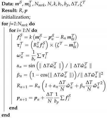
For implementation purposes the psuedocode is presented in Algorithm 1:
| Algorithm 1:Damped least square algorithm for the filtering motion tracker’s signal. |
 |
2.2. Experimental Verification of the Filtered Motion Capture Signal
Measuring Object’s position: To test and validate the filter, eight optical markers are attached to a rigid object (see Figure 1). Four additional markers from the origin of the global coordinate frame . The position of the markers is defined via the computer-aided design (CAD) drawing. The object is moved randomly involving translations and rotations with the motion capture system tracking at 50 Hz. All markers are visible during this experiment. To verify the filter algorithm, the position data of four markers is manually manipulated i.e., the markers 3rd can be considered invisible to the camera system for a continuous time of 20s. Figure 3 shows that the complementary filter can reconstruct the missing markers. The experimental test to verify the damped least square filter algorithm is presented in [20].
3. Complementary Filter on
In the previous section, a model is developed to filter the motion capture data. The motion capture can detect large rotations and translations at low frequencies, but micro-motions may stay undetected when the amplitudes are too small and the frequencies too high. This section proposes an algorithm capable to capture both the micro- and macro-motions on .
Complementary filters traditionally apply when redundant measurements are available [26] and combining all available information in order to minimize the instrumentation error. They are also used to fuse information from multiple sensors and correct the output based on the sensed inputs. Although the Kalman filters can be extended (EKF) to nonlinear cases, they fail in capturing the nonlinear structure (e.g., rotations of a rigid body) which can be detected using complementary filters [13,14,15,27]. Therefore, the question arises how to properly measure micro-motions that are characterized by small amplitudes and high frequencies. IMUs can be used to measure orientations, accelerations, and the magnetic field.
Both the IMUs and motion capture can detect the orientation of an object in space. While motion capture system have high 3D resolution at reasonably high acquisition frequency they are outperformed by IMU in terms of temporal and technical resolution. Accelerometers and gyroscopes may have high temporal resolution but are known to show signal drift over time. A combination of both systems could improve the acquisition of slow major movements (3D motion capture) and micro-motions (IMUs) at the same time.
3.1. High-Frequency Motion Capture Imu Sensor Specifications
In this paper, a customized IMU described in the following is used together with motion capture to improve the acquisition of slow major movements (3D motion capture) and micro-motions simultaneously. The IMU sensor unit is mainly composed by (i) a 9-axis magneto-inertial sensor, the LSM9DS0 manufactured by STmicroelectronics, Inc., which embeds 3 axial accelerometers, gyroscopes and magnetometers. The LSM9DS0 is designed with a small outline (a 4 × 4 mm LGA24 package) and provides digital access to sensor data via I2C serial communication; (ii) a 16-bit microcontroller, the dsPIC33FJ64GP202 by Microchip, Inc., which collects the data from the sensor, and sends it to the Bluetooth module for wireless transmission. The microcontroller also processes the data with a quaternion-based complementary filter [28] in order to estimate the 3D orientation of the sensor, and transmits both raw data and computed quaternions with a sampling frequency of 200 Hz; (iii) a Bluetooth module, the SPBT2632C2A, by STmicroelectronics, Inc., guarantees the wireless communication from the sensor unit to a remote laptop via a Virtual COM Port (VCP); (iv) a rechargeable Li-Po battery with a capacity of 260 mAh, which assures the power supply with at least 4 h of continuous data streaming. The overall dimensions of the IMU sensor unit are 35 × 35 × 22 mm (see Figure 4).
3.2. Complementary Filter
Based on the complementary filter on for dynamic attitude estimation presented by Campolo et al. [23], the measurement inputs are the rigid body orientation obtained from the motion capture system and the angular velocity measured by the IMU to estimate the kinematics of the rigid object on . An experimental validation is proposed to verify the filter algorithm will be presented in the next section. The following identities are used.
- The rotation and denotes the relative orientation of the instrumented box with respect to the global frame which is measured by using, respectively, the motion tracker and IMU.
- Vectors presents the translation of frame in global frame .
- denotes the angular velocity of the rigid object measured by the IMU.
- denotes the output of the accelerometers embedded in the IMU and are expressed in moving frame coordinates.
- denotes the oscillation force which is caused by the plate of the loadcell.
Given a rigid object with a defined object frame , the rotation measured by using the motion tracker presents the relative orientation of the rigid object frame with respect to the global frame . The gray block (i) in Figure 5 shows how raw data from motion capture are geometrically preprocessed to generate a filtered output to be fused with IMU angular velocity . Such a sensor fusion takes place in the complementary filter shown in the block (ii) in Figure 5. Specifically, the rotation represents the estimated orientation of the rigid object and is defined by the following time-continuous equations,
where k is the only gain and, as in any complementary filter, it can be optimally tuned based on the noise characteristics of the signal [26].
So far, direct integration of angular velocities led to a estimation of complementing the existing estimate from motion capture. Data from accelerometers , however, cannot be directly integrated because they are expressed in a moving frame and, further more, contain a gravitational bias (In Figure 5, this is expressed by the additional gray-color term , where R is the actual (and unknown) 3D body orientation, estimated by . Because of estimation errors, is not exactly the identity matrix, this is expressed by the “tilde” variable which is supposed to be close to .). By means of the 3D orientation estimates , accelerations can be transformed in space-fixed coordinates, where the gravitational bias can be simply subtracted:
as shown in the non-gray area in Figure 5. It should be noted that the gravitational bias is contact in space-fixed frame and equal to m/s.
At this point, the space-fixed accelerations (without biased) could be directly integrated with respect to time to produce an estimate of linear velocities . A second integration, in cascade, would lead to an estimation of space-fixed positions . However, errors in the estimations of the gravitational bias (directly due to attitude errors in ) and noise would rapidly lead to a drift of such estimates, in typically rapid time. In order to limit the drift by fusing positions as estimated from the motion capture. The cascade of linear, complementary filter to derive velocity and position estimates is shown in block (iii) of Figure 5.
4. Experimental Verification
In this section, the ability of the proposed complementary filter to detect both micro-motions and macro- motions will be demonstrated experimentally. On the one hand, micro-motions entail small amplitude but high-frequency content which is typical of vibratory phenomena. To this end, a 6-degrees of freedom (dof) loadcell will be used as ground-truth to detect accelerations induced by the vibratory phenomena. On the other hand, macro-motions entail large amplitude but low frequency kinematics which is easily detected via motion trackers. We shall show that by fusing both motion-tracking information as well as accelerometers, a complementary filter is able to reliably detect both micro- and macro- motions.
Although the filter structure in Section 2 is general and application-independent, the specific hardware (motion tracker and IMU) along with specific sampling rates, reflects applications involving human motion. In particular, targeting human activities of daily living, the instrumented object was mounted on a leaf-spring and held by one of the authors while performing arbitrary, oscillatory hand-motions. Such motions are deemed representative of activities of daily leaving. The leaf spring mechanism was used to amplify natural and comfortable hand motions, at least in one direction.
Throughout the experimental condition the IMU, motion capture and loadcell recorded the movement (for more information and animations readers are referred to the supplementary data online). The instrumented object is mounted on a leaf spring allowing only rotations as shown in Figure 6. In this set-up, the instrumented object is attached to a leaf spring fixed to a base. The leaf spring is activated and oscillates until it gets back to its neutral position. Then, the whole setup is moved in space to allow both translations and rotations. In order to validate the complementary filter algorithm, the sampling frequency was set to: 200 Hz, 50 Hz, and 1000 Hz for the IMU, motion capture, and load cell, respectively.
The motion capture acquisition frequency was purposely set to 50 Hz to prove the concept of the complementary filter. The filter algorithm is able to detect the movements which the motion capture cannot such as the vibration with high frequencies and small amplitudes. Motion capture can detect large rotations and translations at lower frequencies but micro-motions may stay undetected when the amplitudes are too small and the frequencies too high.
The measured force of the loadcell is the result of the acceleration and its moments of inertia. They are given by the hardware specifications and a multiplication with the estimated accelerations from the complementary filter will allow us to compare the estimated force with the measured force from the loadcell (see Equation (20)).
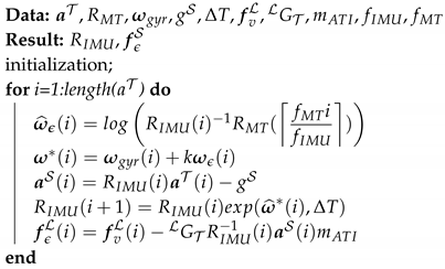
Equation (Section 3.2) is time-continuous and any solution starting on is guaranteed to remain on . However, this would no longer be the case if (Section 3.2) were to be directly discretized, e.g., by a numerical simulator, and the solution will likely drift away from . Campolo et al. [23] proposed a technique that avoids this phenomenon and the following pseudocode in Algorithm 2 describes a possible numerical implementation,
where 200 Hz, 50 Hz is the sampling frequency of the IMU and motion capture, respectively; the notation denotes the ceiling function maps a real number to the smallest following integer.
| Algorithm 2:Complementary filter algorithm on . |
 |
The complementary filter uses the motion capture data as reference for the IMU (Figure 5). After each experiment, the estimated acceleration are multiplied with the moments of inertia of the loadcell and compared with the measured forces. The moments inertia of the plate of the ATI mini40 loadcell are
An estimated force from the complementary filter is defined as
where is an homogeneous transformation matrix computed from the CAD of the instrumented box. Therefore, the error between the measured force by loadcell and the estimated force by the complementary filter in the loadcell frame can be determined as
Figure 7 shows how well the estimated forces match the force detected by the loadcell . A linear regression of measured forces vs. estimated forces resulted in a goodness of fit with R-squared of , , and for the x-, y-, and z-components, respectively.
Bland–Altman plots [29] were computed to analyze the agreement between the estimated and the measured forces, as shown in Figure 8. Furthermore, the determination coefficient (r2) and the squared sum errors (SSE) were computed for each experiment and each force direction (Fx, Fy, Fz) to measure the discrepancy between the estimated and measured forces. The experimental results show strong coherence and small discrepancy between the estimated and measured forces. The direct comparison between the estimated and measured force shows quasi-linear relationship across all conditions. The complementary filter increases the accuracy of the estimated values of acceleration.
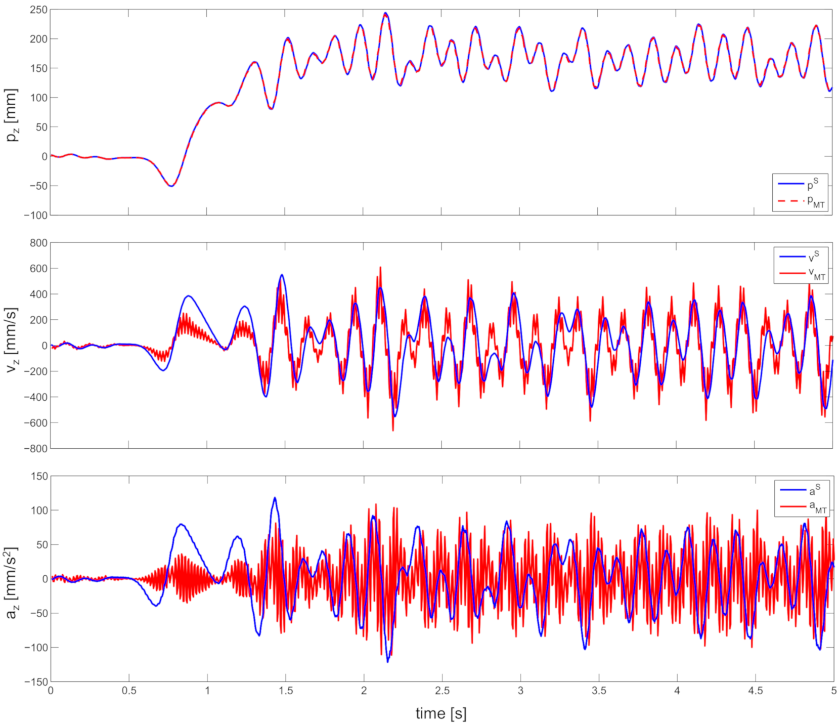
Finally, Figure 9 shows a comparison of z-axis position, velocity, and accelerations as detected by the motion tracker and as estimated by the filter in Figure 5. While position estimates are almost indistinguishable (R-squared when MT positions data are linearly regressed with IMU position estimates), a decay in similarity can be seen when comparing velocities (R-squared ) and even more when it comes to accelerations (R-squared ).
5. Conclusions
In this paper, we have discussed the integration of two measurement systems to detect micro- and macro-motions. Multimodal sensor fusion is conducted using a complementary filter specialized to the nonlinear structure of the group of rigid body rotations. This work aimed to improve the estimation of acceleration, free from gravitational bias using a complementary filter. Both the numerical implementation and the experimental validation have been provided as a verification and to complement the theoretical approach. The proposed filter was experimentally tested and validated based on the force measurements from a loadcell.
Optical and IMU technologies can be either used as standalone systems for specific applications but the strength lies in the their combination to deepen our understanding of movement assessment. Optical technology has traditionally been used to the laboratory setting; inertial technology takes movement analysis out to the field. As such, the combination of optical and inertial technologies will contribute to the performance assessments both in sports and industrial tasks.
Author Contributions
Conceptualization, G.-H.P., C.H., P.T., A.H., D.F. and D.C.; Data curation, A.H.; Formal analysis, G.-H.P., C.H.; Methodology, P.T., A.B., and D.C.; Resources, D.C.; Software, P.T.; Supervision, A.H., D.F. and D.C.; Validation, D.F. and D.C.; Visualization, C.H.; Writing—original draft, G.-H.P., C.H., and D.C.; Writing—review & editing, G.-H.P., C.H., P.T., A.H., D.F. and D.C. All authors have read and agreed to the published version of the manuscript.
Funding
The work was supported by the Tier 1 project (RG 48/17), MOE, Singapore. This research is funded by Ho Chi Minh City University of Technology (HCMUT), VNUHCM under grant number HCMUT-003967-2020. We acknowledge financial support by DFG within the funding programme Open Access Publizieren.
Conflicts of Interest
The authors declare no conflict of interest.
References
- Beecks, C.; Hassani, M.; Brenger, B.; Hinnell, J.; Schüller, D.; Mittelberg, I.; Seidl, T. Efficient query processing in 3D motion capture gesture databases. Int. J. Semant. Comput. 2016, 10, 5–25. [Google Scholar] [CrossRef] [Green Version]
- Lim, C.K.; Luo, Z.; Chen, I.M.; Yeo, S.H. A low cost wearable optical-based goniometer for human joint monitoring. Front. Mech. Eng. 2011, 6, 13–22. [Google Scholar] [CrossRef]
- Mayagoitia, R.E.; Nene, A.V.; Veltink, P.H. Accelerometer and rate gyroscope measurement of kinematics: An inexpensive alternative to optical motion analysis systems. J. Biomech. 2002, 35, 537–542. [Google Scholar] [CrossRef]
- Takeda, R.; Tadano, S.; Natorigawa, A.; Todoh, M.; Yoshinari, S. Gait posture estimation using wearable acceleration and gyro sensors. J. Biomech. 2009, 42, 2486–2494. [Google Scholar] [CrossRef] [PubMed] [Green Version]
- Chung, P.; Ng, G. Comparison between an accelerometer and a three-dimensional motion analysis system for the detection of movement. Physiotherapy 2012, 98, 256–259. [Google Scholar] [CrossRef] [PubMed]
- Stone, J.; Currier, B.; Niebur, G.; An, K.N. The use of a direct current electromagnetic tracking device in a metallic environment. Biomed. Sci. Instrum. 1995, 32, 305–311. [Google Scholar]
- Perie, D.; Tate, A.; Cheng, P.; Dumas, G. Evaluation and calibration of an electromagnetic tracking device for biomechanical analysis of lifting tasks. J. Biomech. 2002, 35, 293–297. [Google Scholar] [CrossRef]
- Bull, A.; Berkshire, F.; Amis, A. Accuracy of an electromagnetic measurement device and application to the measurement and description of knee joint motion. Proc. Inst. Mech. Eng. Part H J. Eng. Med. 1998, 212, 347–355. [Google Scholar] [CrossRef] [PubMed]
- Phan, G.H.; Hansen, C.; Tommasino, P.; Budhota, A.; Mohan, D.M.; Hussain, A.; Burdet, E.; Campolo, D. Estimating Human Wrist Stiffness during a Tooling Task. Sensors 2020, 20, 3260. [Google Scholar] [CrossRef] [PubMed]
- Lasenby, J.; Stevenson, A. Using geometric algebra for optical motion capture. In Geometric Algebra with Applications in Science and Engineering; Springer: Berlin/Heidelberg, Germany, 2001; pp. 147–169. [Google Scholar]
- De Canio, G.; de Felice, G.; De Santis, S.; Giocoli, A.; Mongelli, M.; Paolacci, F.; Roselli, I. Passive 3D motion optical data in shaking table tests of a SRG-reinforced masonry wall. Earthquakes Struct. 2016, 40, 53–71. [Google Scholar] [CrossRef]
- Filippeschi, A.; Schmitz, N.; Miezal, M.; Bleser, G.; Ruffaldi, E.; Stricker, D. Survey of motion tracking methods based on inertial sensors: A focus on upper limb human motion. Sensors 2017, 17, 1257. [Google Scholar] [CrossRef] [PubMed] [Green Version]
- Campolo, D.; Keller, F.; Guglielmelli, E. Inertial/magnetic sensors based orientation tracking on the group of rigid body rotations with application to wearable devices. In Proceedings of the 2006 IEEE/RSJ International Conference on Intelligent Robots and Systems, Beijing, China, 9–15 October 2006; pp. 4762–4767. [Google Scholar]
- Mahony, R.; Hamel, T.; Pflimlin, J.M. Nonlinear complementary filters on the special orthogonal group. IEEE Trans. Autom. Control 2008, 53, 1203–1218. [Google Scholar] [CrossRef] [Green Version]
- Campolo, D.; Schenato, L.; Pi, L.; Deng, X.; Guglielmelli, E. Attitude estimation of a biologically inspired robotic housefly via multimodal sensor fusion. Adv. Robot. 2009, 23, 955–977. [Google Scholar] [CrossRef]
- Jung, H.H.; Kim, M.K.; Lyou, J. Realization of a hybrid human motion capture system. In Proceedings of the 2017 17th International Conference on Control, Automation and Systems (ICCAS), Jeju, Korea, 18–21 October 2017; pp. 1581–1585. [Google Scholar]
- Vergara, M.; Sancho, J.L.; Rodríguez, P.; Pérez-González, A. Hand-transmitted vibration in power tools: Accomplishment of standards and users’ perception. Int. J. Ind. Ergon. 2008, 38, 652–660. [Google Scholar] [CrossRef]
- Zheng, Z.; Yu, T.; Li, H.; Guo, K.; Dai, Q.; Fang, L.; Liu, Y. Hybridfusion: Real-time performance capture using a single depth sensor and sparse imus. In Proceedings of the European Conference on Computer Vision (ECCV), Munich, Germany, 8–14 September 2018; pp. 384–400. [Google Scholar]
- Guzsvinecz, T.; Szucs, V.; Sik, C.L. Developing movement recognition application with the use of Shimmer sensor and Microsoft Kinect sensor. Stud. Health Technol. Inform. 2015, 217, 767–772. [Google Scholar] [PubMed]
- Gia Hoang, P.; Asif, H.; Campolo, D. Preparation for capturing human skills during tool. In Applied Mechanics and Materials; Trans Tech: Warwick, NY, USA, 2016; Volume 842, pp. 293–302. [Google Scholar]
- Dorfmüller-Ulhaas, K. Robust optical user motion tracking using a kalman filter. In Proceedings of the 10th ACM Symposium on Virtual Reality Software and Technology, Osaka, Japan, 1–3 October 2003. [Google Scholar]
- Welch, G.; Bishop, G.; Vicci, L.; Brumback, S.; Keller, K.; Colucci, D.N. The HiBall tracker: High-performance wide-area tracking for virtual and augmented environments. In Proceedings of the ACM Symposium on Virtual Reality Software and Technology, London, UK, 20–22 December 1999. [Google Scholar]
- Campolo, D.; Schenato, L.; Pi, L.; Deng, X.; Guglielmelli, E. Multimodal sensor fusion for attitude estimation of micromechanical flying insects: A geometric approach. In Proceedings of the IEEE/RSJ International Conference on Intelligent Robots and Systems, Nice, France, 22–26 September 2008; pp. 3859–3864. [Google Scholar]
- Baldwin, G.; Mahony, R.; Trumpf, J.; Hamel, T.; Cheviron, T. Complementary filter design on the Special Euclidean group SE (3). In Proceedings of the 2007 European Control Conference (ECC), Kos, Greece, 2–5 July 2007; pp. 3763–3770. [Google Scholar]
- Murray, R.M.; Li, Z.; Sastry, S.S. A Mathematical Introduction to Robotic Manipulation; CRC Press: Boca Raton, FL, USA, 1994. [Google Scholar]
- Brown, R.G.; Hwang, P.Y. Introduction to random signals and applied Kalman filtering: With MATLAB exercises and solutions. In Introduction to Random Signals and Applied Kalman Filtering: With MATLAB Exercises and Solutions; Brown, R.G., Hwang, P.Y.C., Eds.; Wiley: New York, NY, USA, 1997; Volume 1. [Google Scholar]
- Daum, F. Nonlinear filters: Beyond the Kalman filter. Aerosp. Electron. Syst. Mag. IEEE 2005, 20, 57–69. [Google Scholar] [CrossRef]
- Madgwick, S.O.; Harrison, A.J.; Vaidyanathan, R. Estimation of IMU and MARG orientation using a gradient descent algorithm. In Proceedings of the 2011 IEEE International Conference Rehabilitation Robotics (ICORR), Zurich, Switzerland, 29 June–1 July 2011; pp. 1–7. [Google Scholar]
- Giavarina, D. Understanding bland altman analysis. Biochem. Med. Biochem. Med. 2015, 25, 141–151. [Google Scholar] [CrossRef] [PubMed] [Green Version]
- Machireddy, A.; Van Santen, J.; Wilson, J.L.; Myers, J.; Hadders-Algra, M.; Song, X. A video/IMU hybrid system for movement estimation in infants. In Proceedings of the 2017 39th Annual International Conference of the IEEE Engineering in Medicine and Biology Society (EMBC), Seogwipo, Korea, 11–15 July 2017; pp. 730–733. [Google Scholar]
- Phan, G.H.; Hansen, C.; Tommasino, P.; Hussain, A.; Campolo, D. Design and characterization of an instrumented hand-held power tool to capture dynamic interaction with the workpiece during manual operations. Int. J. Adv. Manuf. Technol. 2020, 111, 1–14. [Google Scholar] [CrossRef]
- Phan, G.H.; Tommasino, P.; Hussain, A.; Hansen, C.; Castagne, S.; Campolo, D. Geometry of contact during tooling tasks via dynamic estimation. Int. J. Adv. Manuf. Technol. 2018, 94, 2895–2904. [Google Scholar] [CrossRef]
Figure 1.
Conceptual design of the instrumented box: a loadcell attached on the top of the box; the inertial measurement unit (IMU) is located inside, at the center while the infrared markers allow capturing 3D position and orientation of the box. Attaching markers on the top and side of the tool. Assuming that the marker’s position on the tool is known from the computer-aided design (CAD) drawing.
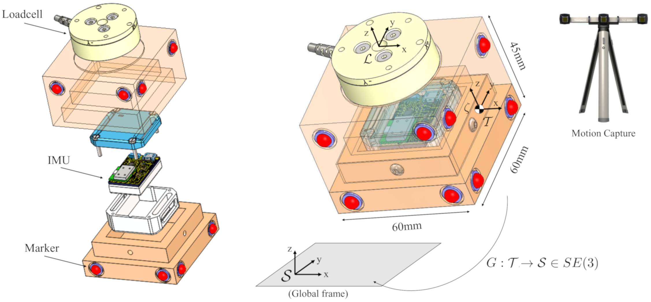
Figure 2.
Spring-Markers system: In a time interval, the different between the position estimated and position from CAD of each marker cause the force pull the tool back to the right position.
Figure 2.
Spring-Markers system: In a time interval, the different between the position estimated and position from CAD of each marker cause the force pull the tool back to the right position.
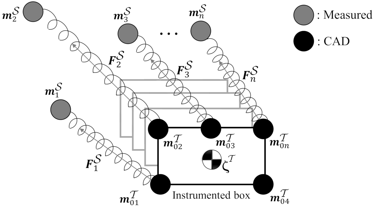
Figure 3.
(a) Marker 3rd is invisible in 20 s and (b) Marker 6th is visible. Estimated marker position based on the complementary filter in x, y and z-direction.
Figure 3.
(a) Marker 3rd is invisible in 20 s and (b) Marker 6th is visible. Estimated marker position based on the complementary filter in x, y and z-direction.
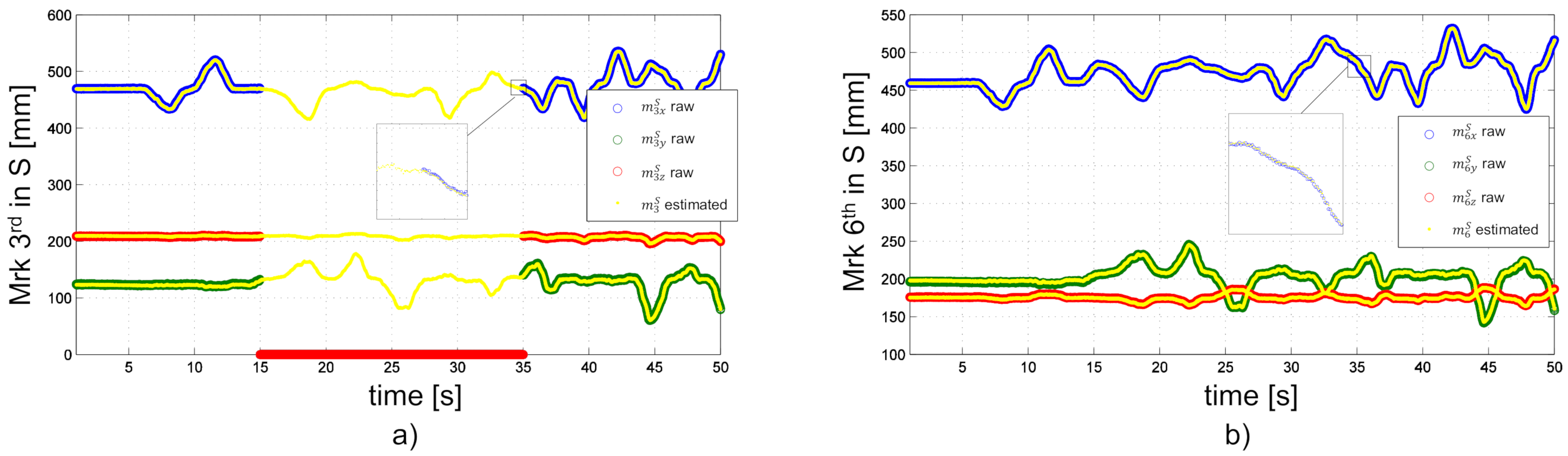
Figure 4.
The IMU sensor unit.
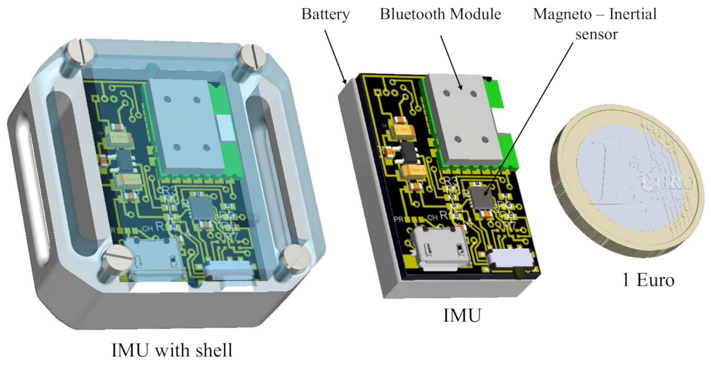
Figure 5.
complementary filter used to estimate 3D orientation as well as space-frame positions , velocities , and accelerations from motion tracker (MT) and IMU raw data. The three gray blocks represent a low-pass filter on , a nonlinear complementary filter combining low-pass filtered 3D orientations from the motion tracker with angular velocities from the gyroscopes, and a cascade of two linear complementary filters to estimate space-fixed velocities and positions from space-fixed accelerations. The operations outside of the gray boxes simply represent body-frame accelerations into space-frame accelerations from the constant the gravitational bias can be simply subtracted.
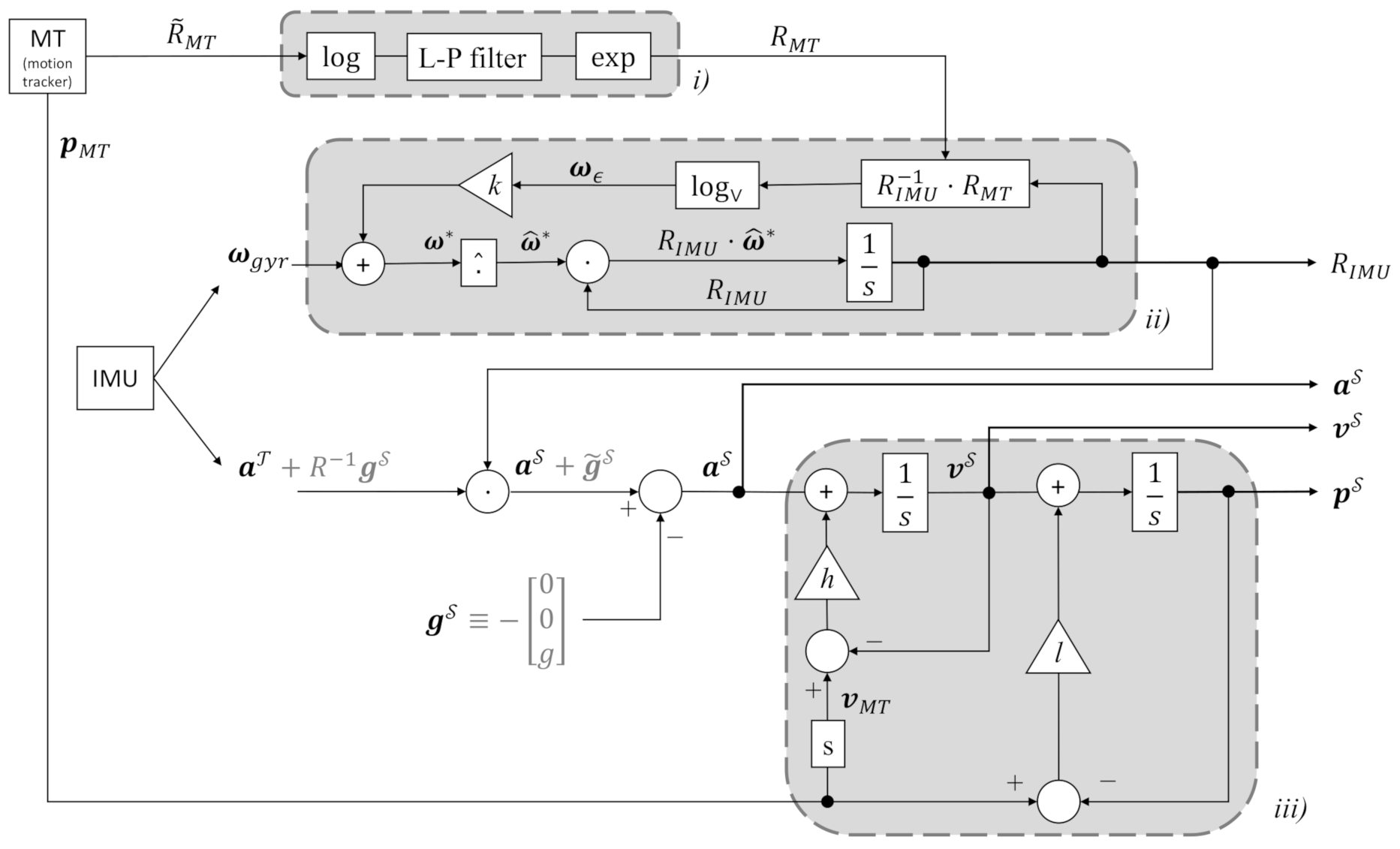
Figure 6.
Experimental conditions: Translation and Rotation.
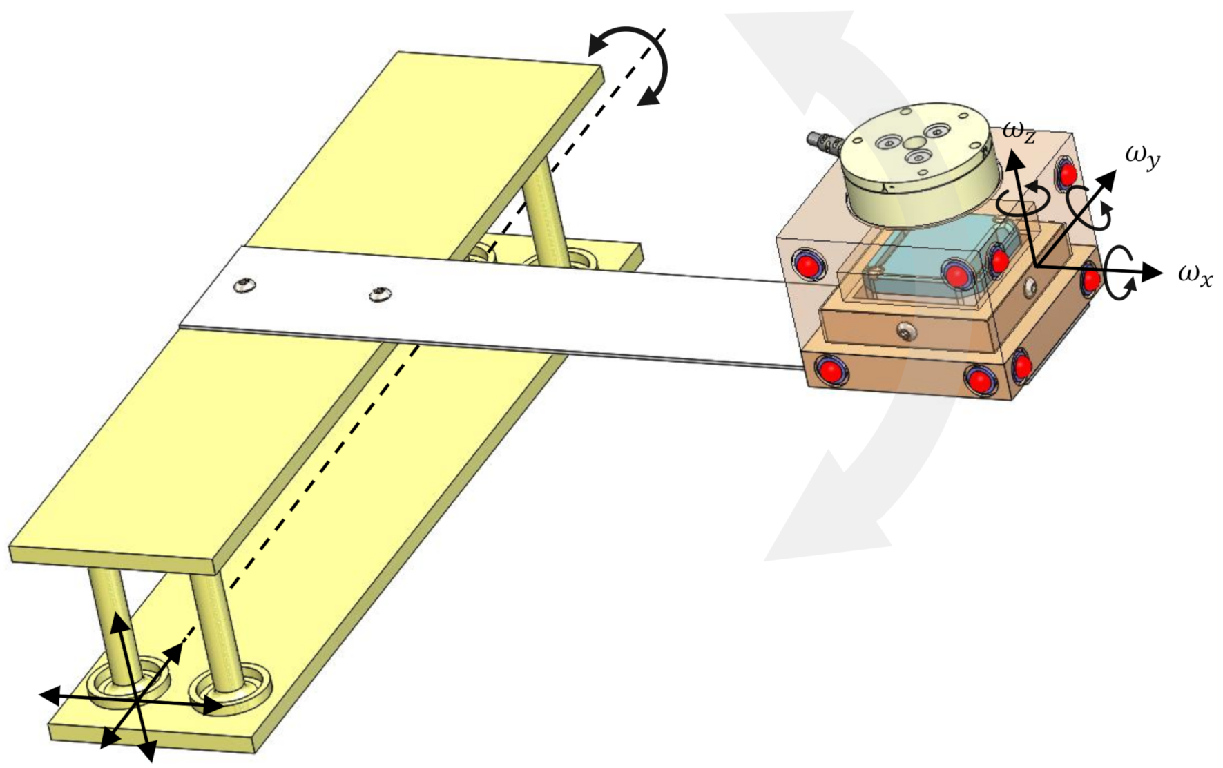
Figure 7.
Component-wise comparison of forces as measured from the loadcell and non-inertial forces as estimated through IMU accelerations.
Figure 7.
Component-wise comparison of forces as measured from the loadcell and non-inertial forces as estimated through IMU accelerations.
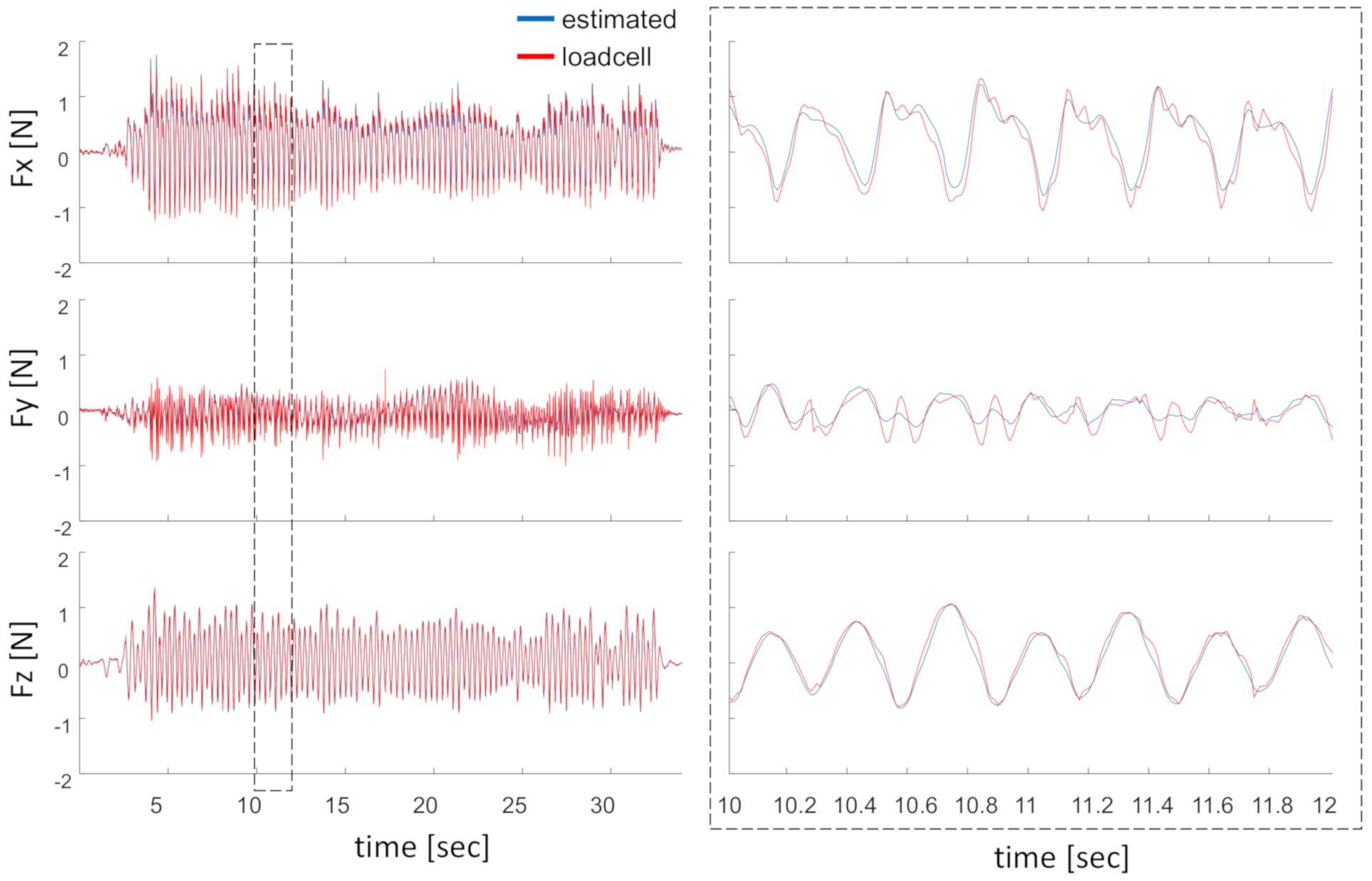
Figure 8.
Comparison of the experimental and computed forces (Fx, Fy, Fz) throughout the 34 s experiment (number of data points n = 3401) show strong coherence and small discrepancy between the estimated and measured forces.
Figure 8.
Comparison of the experimental and computed forces (Fx, Fy, Fz) throughout the 34 s experiment (number of data points n = 3401) show strong coherence and small discrepancy between the estimated and measured forces.
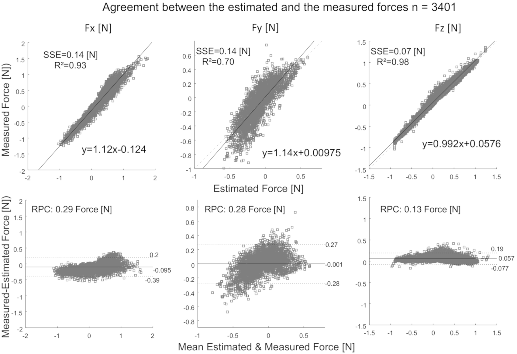
Figure 9.
The position and acceleration of the instrumented box in z axis (direction with largest motion).
Figure 9.
The position and acceleration of the instrumented box in z axis (direction with largest motion).
Publisher’s Note: MDPI stays neutral with regard to jurisdictional claims in published maps and institutional affiliations. |
© 2020 by the authors. Licensee MDPI, Basel, Switzerland. This article is an open access article distributed under the terms and conditions of the Creative Commons Attribution (CC BY) license (http://creativecommons.org/licenses/by/4.0/).
Share and Cite
MDPI and ACS Style
Phan, G.-H.; Hansen, C.; Tommasino, P.; Hussain, A.; Formica, D.; Campolo, D. A Complementary Filter Design on SE(3) to Identify Micro-Motions during 3D Motion Tracking. Sensors 2020, 20, 5864. https://doi.org/10.3390/s20205864
AMA Style
Phan G-H, Hansen C, Tommasino P, Hussain A, Formica D, Campolo D. A Complementary Filter Design on SE(3) to Identify Micro-Motions during 3D Motion Tracking. Sensors. 2020; 20(20):5864. https://doi.org/10.3390/s20205864
Chicago/Turabian StylePhan, Gia-Hoang, Clint Hansen, Paolo Tommasino, Asif Hussain, Domenico Formica, and Domenico Campolo. 2020. "A Complementary Filter Design on SE(3) to Identify Micro-Motions during 3D Motion Tracking" Sensors 20, no. 20: 5864. https://doi.org/10.3390/s20205864
Note that from the first issue of 2016, this journal uses article numbers instead of page numbers. See further details here.