Design of 2D Sparse Array Transducers for Anomaly Detection in Medical Phantoms

Abstract
1. Introduction
- Design a 2D array transducer to achieve enhanced and flexible imaging capability.
- Develop an image processing approach to automatically detect anomalies in the blood flow.
2. Design of Sparse Array Pattern
2.1. Sparse Array Configurations
2.1.1. Random Array Pattern
2.1.2. Sunflower Spiral Array Pattern
2.1.3. Log Spiral Array Pattern
2.2. Peak Sidelobe Level (PSL) and Integrated Sidelobe Ratio (ISLR)
2.3. Simulation Process and Results
3. Transducer Manufacturing and Characterisation
3.1. Fabrication of Prototype Transducers
3.2. Impedance Response
3.3. Inter-Element Cross-Talk
3.4. Pulse-Echo Response
4. Particle Detection Algorithm
5. System Evaluation
5.1. Imaging Tube-Tank Phantom
5.2. Imaging TMM Phantom
6. Conclusions
Author Contributions
Funding
Acknowledgments
Conflicts of Interest
References
- Demchuk, A.; Menon, B.; Goyal, M. Comparing Vessel Imaging Noncontrast Computed Tomography/Computed Tomographic Angiography Should Be the New Minimum Standard in Acute Disabling Stroke. Stroke 2016, 47, 273–281. [Google Scholar] [CrossRef] [PubMed]
- Feldman, M.; Katyal, S.; Blackwood, M. US Artifacts. RadioGraphics 2009, 29, 1179–1189. [Google Scholar] [CrossRef] [PubMed]
- Tsivgoulis, G.; Alexandrov, A. Ultrasound-enhanced thrombolysis in acute ischemic stroke: Potential, failures, and safety. Neurotherapeutics 2007, 4, 420–427. [Google Scholar] [CrossRef] [PubMed]
- Steinberg, B. Principles of Aperture and Array Systems Design; Wiley: New York, NY, USA, 1976; p. 54. [Google Scholar]
- Tweedie, A. Spiral 2D Array Designs for Volumetric Imaging. Ph.D. Thesis, University of Strathclyde, Glasgow, UK, 2011. [Google Scholar]
- Choe, J.W.; Oralkan, Ö.; Khuri-Yakub, P.T. Design optimization for a 2-D sparse transducer array for 3-D ultrasound imaging. In Proceedings of the 2010 IEEE International Ultrasonics Symposium, San Diego, CA, USA, 11–14 October 2010. [Google Scholar]
- Yang, P.; Chen, B.; Shi, K. A novel method to design sparse linear arrays for ultrasonic phased array. Ultrasonic 2006, 44, e717–e721. [Google Scholar] [CrossRef] [PubMed]
- Moffet, A. Minimum-redundancy linear arrays. IEEE Trans. Antennas Propag. 1968, 16, 172–175. [Google Scholar] [CrossRef]
- Ramalli, A.; Boni, E.; Savoia, A.; Tortoli, P. Density-tapered spiral arrays for ultrasound 3-D imaging. IEEE Trans. Ultrason. Ferroelectr. Freq. Control 2015, 62, 1580–1588. [Google Scholar] [CrossRef] [PubMed]
- Diarra, B.; Robini, M.; Tortoli, P.; Cachard, C.; Liebgott, H. Design of Optimal 2-D Nongrid Sparse Arrays for Medical Ultrasound. IEEE Trans. Biomed. Eng. 2013, 60, 3039–3102. [Google Scholar] [CrossRef] [PubMed]
- Diarra, B.; Roux, E.; Liebgott, H.; Ravi, S.; Robini, M.; Tortoli, P.; Cachard, C. Comparison of different optimized irregular sparse 2D ultrasound arrays. In Proceedings of the 2016 IEEE International Ultrasonics Symposium, Tours, France, 18–21 September 2016. [Google Scholar]
- Viganó, M.; Toso, G.; Caille, G.; Mangenot, C.; Lager, I. Sunflower Array Antenna with Adjustable Density Taper. Int. J. Antennas Propag. 2009, 2009, 1–10. [Google Scholar] [CrossRef]
- Martínez-Graullera, O.; Martín, C.; Godoy, G.; Ullate, L. 2D array design based on Fermat spiral for ultrasound imaging. Ultrasonics 2010, 50, 280–289. [Google Scholar] [CrossRef] [PubMed]
- Yoon, H.; Song, T. Sparse Rectangular and Spiral Array Designs for 3D Medical Ultrasound Imaging. Sensors 2019, 20, 173. [Google Scholar] [CrossRef] [PubMed]
- Lethiecq, M.; Levassort, F.; Certon, D.; Tran-Huu-Hue, L. Piezoelectric Transducer Design for Medical Diagnosis and NDE. In Piezoelectric and Acoustic Materials for Transducer Applications, 1st ed.; Safari, A., Akdogan, E., Eds.; Springer: New York, NY, USA, 2008; pp. 191–215. [Google Scholar]
- Harvey, G.; Gachagan, A.; Mackersie, J.; Mccunnie, T.; Banks, R. Flexible ultrasonic transducers incorporating piezoelectric fibres. IEEE Trans. Ultrason. Ferroelectr. Freq. Control 2009, 56, 1999–2009. [Google Scholar] [CrossRef] [PubMed]
- Ivancevich, N.; Dahl, J.; Trahey, G.; Smith, S. Phase-aberration correction with a 3-D ultrasound scanner: Feasibility study. IEEE Trans. Ultrason. Ferroelectr. Freq. Control 2006, 53, 1432–1439. [Google Scholar] [CrossRef] [PubMed]
- Ivancevich, N.M. 7A-5 Real-Time 3D Contrast-Enhanced Transcranial Ultrasound. In Proceedings of the 2007 IEEE Ultrasonics Symposium, New York, NY, USA, 28–31 October 2007. [Google Scholar]
- Lindsey, B.; Light, E.; Nicoletto, H.; Bennett, E.; Laskowitz, D.; Smith, S. The ultrasound brain helmet: New transducers and volume registration for in vivo simultaneous multi-transducer 3-D transcranial imaging. IEEE Trans. Ultrason. Ferroelectr. Freq. Control 2011, 58, 1189–1202. [Google Scholar] [CrossRef] [PubMed]
- Li, X. Design of 2D Sparse Array Transducers for Anomaly Detection associated with a Transcranial Ultrasound System. Ph.D. Thesis, University of Strathclyde, Glasgow, UK, 2020. [Google Scholar]
- Mirko Panozzo Zénere, L.L. Sar Image Quality Assesment. Master’s Thesis, Universidad Nacional de Córdoba, Córdoba, Argentina, 2012. [Google Scholar]
- Steinberg, B. The peak sidelobe of the phased array having randomly located elements. IEEE Trans. Antennas Propag. 1972, 20, 129–136. [Google Scholar] [CrossRef]
- Ziomek, L. Fundamentals of Acoustic Field Theory and Space-Time Signal Processing; CRC Press: Boca Raton, FL, USA, 1995; p. 416. [Google Scholar]
- Dziewierz, J.; Ramadas, S.N.; Gachagan, A.; O’Leary, R.L.; Hayward, G. A 2D Ultrasonic array design incorporating hexagonal-shaped elements and triangular-cut piezocomposite substructure for NDE applications. In Proceedings of the 2009 IEEE International Ultrasonics Symposium, Rome, Italy, 20–23 September 2009. [Google Scholar]
- PZT Fibers. Available online: http://www.smart-material.com/PZTFiber-product-main.html (accessed on 23 January 2017).
- O’Leary, R.L.; Hayward, G.; Smillie, G.; Parr, A.C.S. CUE Materials Database, Version 1.2; University of Strathclyde: Glasgow, UK, 2005. [Google Scholar]
- Savakus, H.P.; Klicker, K.A.; Newnham, R.E. PZT-epoxy piezoelectric transducers: A simplified fabrication procedure. Mater. Res. Bull. 1981, 16, 677–680. [Google Scholar] [CrossRef]
- Hossack, J.; Hayward, G. Finite-element analysis of 1–3 composite transducers. IEEE Trans. Ultrason. Ferroelectr. Freq. Control 1991, 38, 618–629. [Google Scholar] [CrossRef] [PubMed]
- Holmes, C.; Drinkwater, B.; Wilcox, P. Post-processing of the full matrix of ultrasonic transmit–receive array data for non-destructive evaluation. NDT E Int. 2005, 38, 701–711. [Google Scholar] [CrossRef]
- Hough, P. Method and Means for Recognizing Complex Patterns. U.S. Patent 3,069,654, 18 December 1962. [Google Scholar]
- Serra, J. Image Analysis and Mathematical Morphology; Academic Press: London, UK, 1982. [Google Scholar]
- Weir, A.J.; Sayer, R.; Wang, C.; Parks, S. A wall-less poly (vinyl alcohol) cryogel flow phantom with accurate scattering properties for transcranial Doppler ultrasound propagation channels analysis. In Proceedings of the 2015 37th Annual International Conference of the IEEE Engineering in Medicine and Biology Society (EMBC), Milan, Italy, 25–29 August 2015. [Google Scholar]
- International Electrotechnical Commission. Ultrasonics—Flow Measurement Systems—Flow Test Object; IEC: Geneva, Switzerland, 2001. [Google Scholar]
- Blanco, P.; Abdo-Cuza, A. Transcranial Doppler ultrasound in neurocritical care. J. Ultrasound 2018, 21, 1–16. [Google Scholar] [CrossRef] [PubMed]
- Kirsch, J.; Mathur, M.; Johnson, M.; Gowthaman, G.; Scoutt, L. Advances in Transcranial Doppler US: Imaging Ahead. RadioGraphics 2013, 33, E1–E14. [Google Scholar] [CrossRef] [PubMed]
- Kassab, M.Y.; Majid, A.; Farooq, M.U.; Azhary, H.; Hershey, L.A.; Bednarczyk, E.M.; Graybeal, D.F.; Johnson, M.D. BTranscranial Doppler: An Introduction for Primary Care Physicians. J. Am. Board Fam. Med. 2007, 20, 65–71. [Google Scholar] [CrossRef] [PubMed]


| Parameters | Interval | Array Type |
|---|---|---|
| Element radius (ele_r) | 0.7:0.05:1.5 (mm) | All three array configurations |
| Minimum gap between two elements within the array (ele_g) * For the log spiral array, this would be the gap between adjacent elements along the same arm. | 0.2:0.05:1 (mm) | Random and sunflower array |
| 0.4:0.05:1 (mm) | Log spiral array | |
| Number of elements within each log spiral arm (ele_per_arm) | 3:1:10 | Log spiral array |
| Number of log spiral arms (num_of_arm) | 7:2:19 | Log spiral array |
| Constant parameter b | 1.2:0.1:1.5 | Log spiral array |
| Array Type | PSL (dB) | ISLR (dB) |
|---|---|---|
| Random Array | −17.85 | 2.92 |
| Sunflower Spiral Array | −17.38 | 0.58 |
| Log Spiral Array | −19.33 | 2.71 |
| Array Type | CECAT | C1–3 | |
|---|---|---|---|
| (kHz) | 2061 | 2030 | |
| 33.6 | 39.4 | ||
| (kHz) | 2587 | 2440 | |
| 43.5 | 44.5 | ||
| 0.64 | 0.59 | ||
| 0.014 | 0.007 | ||
| Device | Centre Frequency (MHz) | Pulse Length (µs) | Bandwidth (%) | Peak-to-Peak Amplitude (mV) |
|---|---|---|---|---|
| CECAT | 1.95 | 1.72 | 47.44 | 11.17 |
| C1–3 | 1.85 | 2.67 | 30.95 | 16.67 |
| Location | Ball Bearing Real Size | ||
|---|---|---|---|
| 1 mm | 1.5 mm | 2 mm | |
| ) | −12.10 | 0.80 | 13.70 |
| ) | 35.25 | 34.70 | 34.00 |
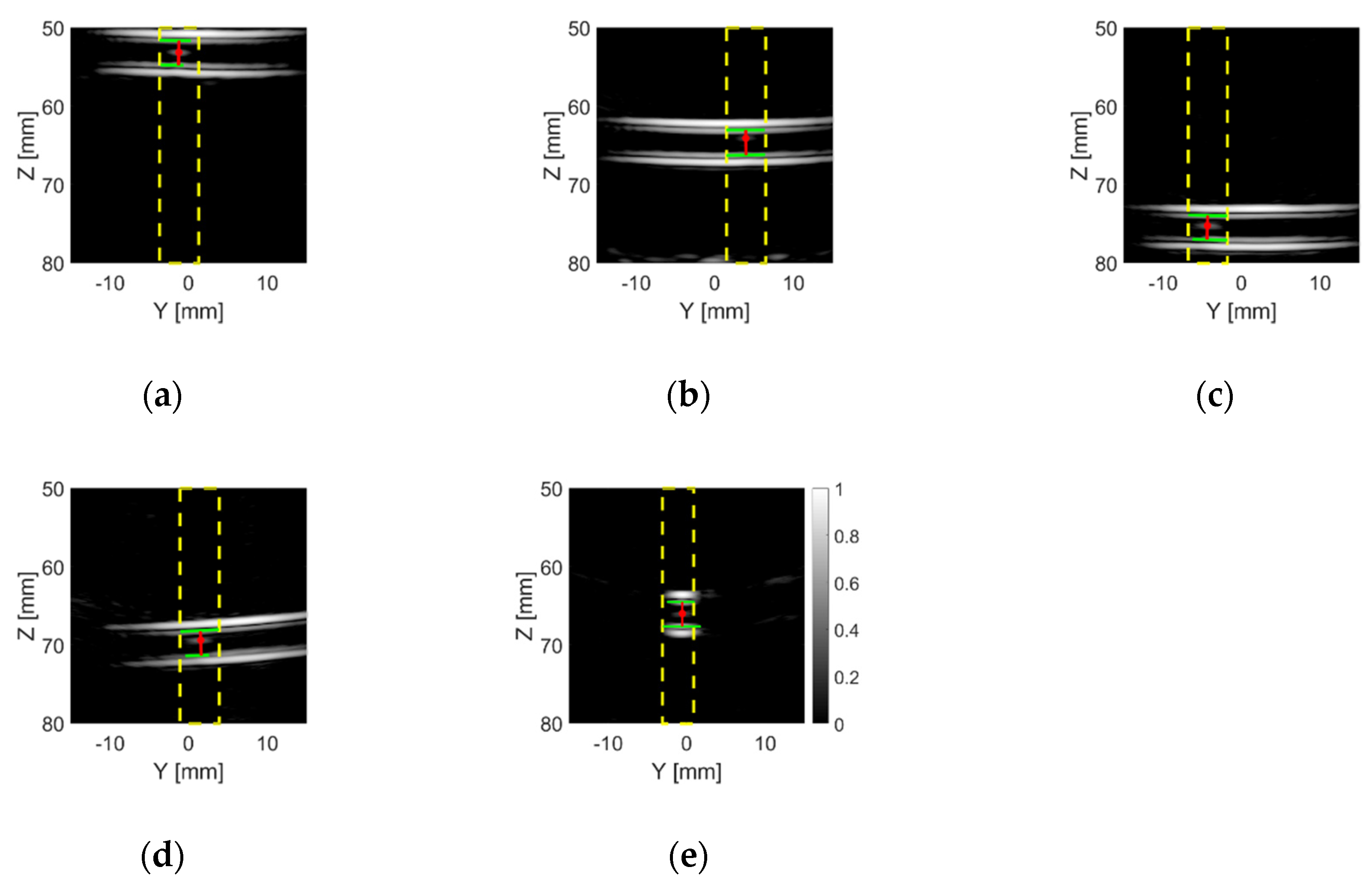
| Phantom Name | Estimated Particle Size (mm) | Estimated Inner Diameter (mm) | Particle Location Pixel Intensity (dB) |
|---|---|---|---|
| 55 mm Phantom | 1.64 | 3.16 | −15.64 |
| 65 mm Phantom | 2.15 | 3.20 | −21.16 |
| 75 mm Phantom | 1.79 | 3.09 | −17.32 |
| Angle V Phantom | 1.93 | 3.16 | −16.90 |
| Angle H Phantom | 1.65 | 3.15 | −21.12 |
© 2020 by the authors. Licensee MDPI, Basel, Switzerland. This article is an open access article distributed under the terms and conditions of the Creative Commons Attribution (CC BY) license (http://creativecommons.org/licenses/by/4.0/).
Share and Cite
Li, X.; Gachagan, A.; Murray, P. Design of 2D Sparse Array Transducers for Anomaly Detection in Medical Phantoms. Sensors 2020, 20, 5370. https://doi.org/10.3390/s20185370
Li X, Gachagan A, Murray P. Design of 2D Sparse Array Transducers for Anomaly Detection in Medical Phantoms. Sensors. 2020; 20(18):5370. https://doi.org/10.3390/s20185370
Chicago/Turabian StyleLi, Xiaotong, Anthony Gachagan, and Paul Murray. 2020. "Design of 2D Sparse Array Transducers for Anomaly Detection in Medical Phantoms" Sensors 20, no. 18: 5370. https://doi.org/10.3390/s20185370
APA StyleLi, X., Gachagan, A., & Murray, P. (2020). Design of 2D Sparse Array Transducers for Anomaly Detection in Medical Phantoms. Sensors, 20(18), 5370. https://doi.org/10.3390/s20185370