Monitoring the Growth and Yield of Fruit Vegetables in a Greenhouse Using a Three-Dimensional Scanner


Abstract
1. Introduction
2. Materials and Methods
2.1. Test Plants and Greenhouse
2.2. Growth Monitoring
2.2.1. Obtaining Point Cloud Data of Plants
2.2.2. Construction of a Surface Model for Growth Estimation
2.3. Yield Monitoring (Tomato and Paprika)
2.3.1. Detection of Fruits from Canopy Point Cloud Data Using RGB Values
2.3.2. Construction of a Solid Model for Estimation of Fruit Weight
3. Results
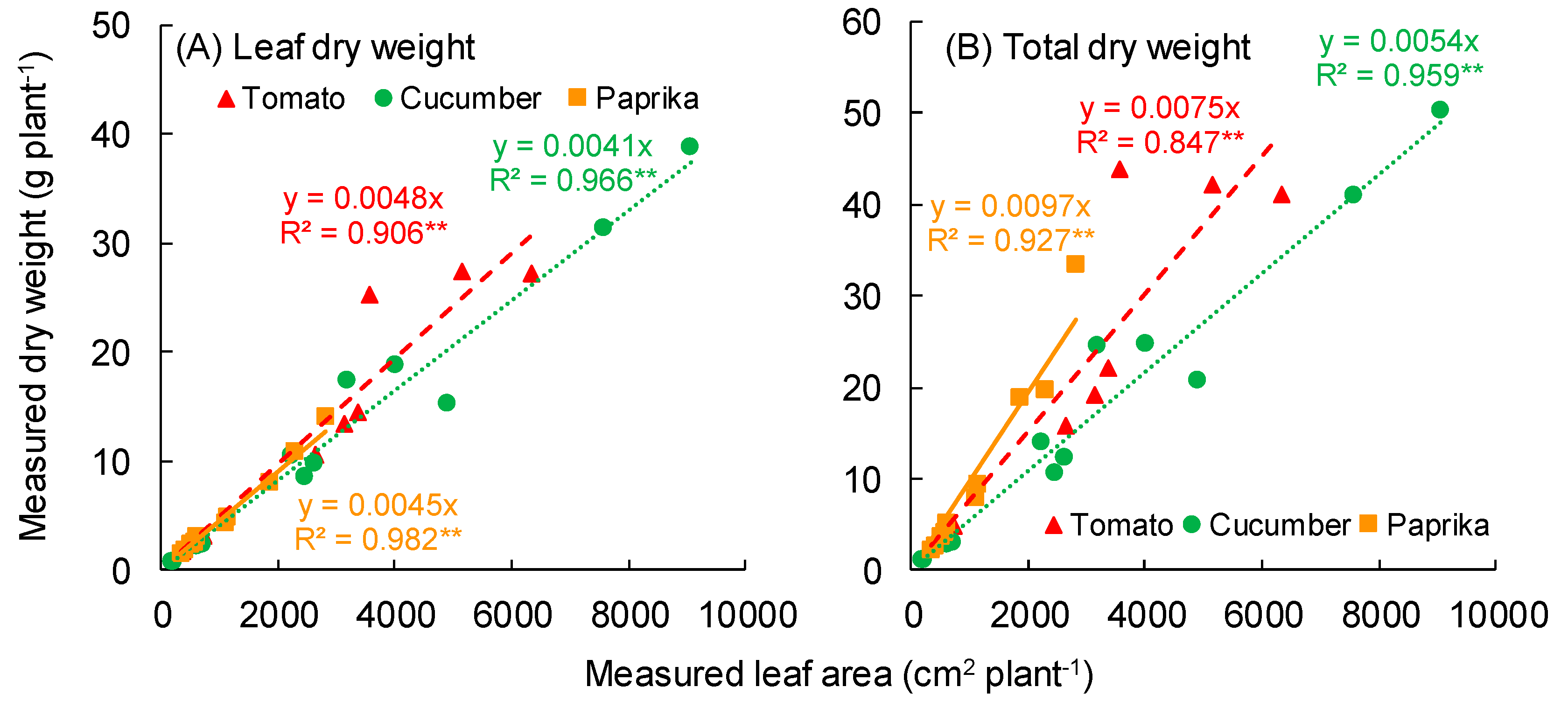
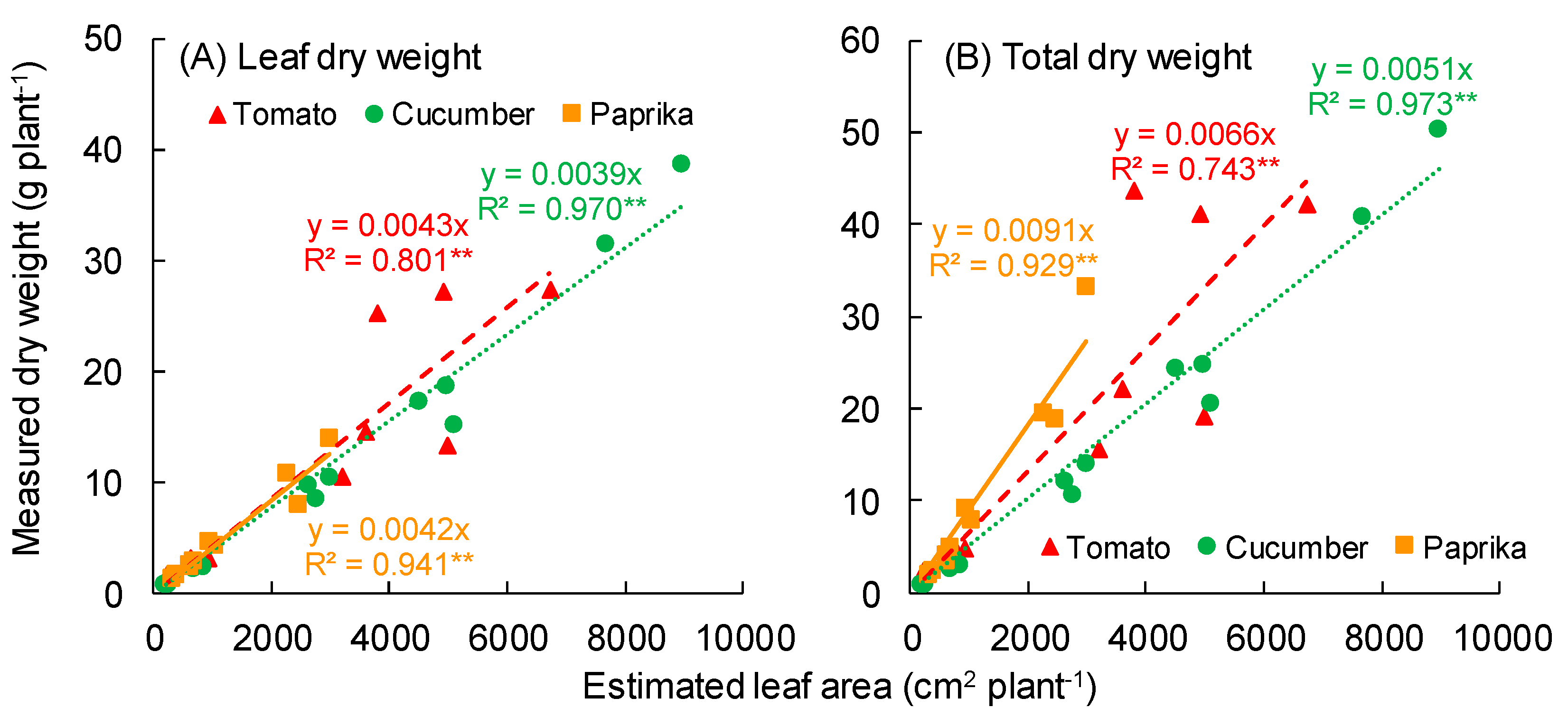
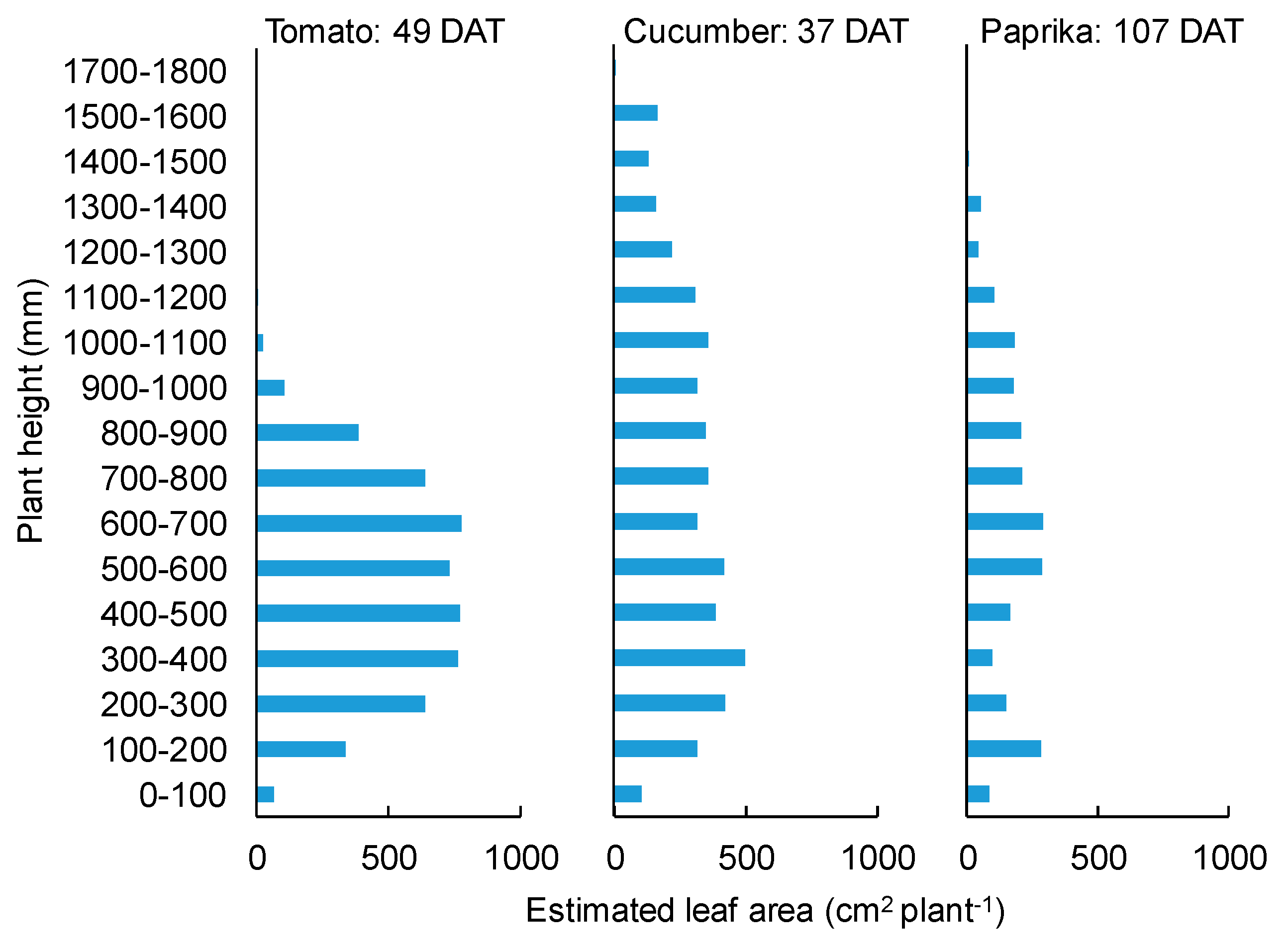
3.1. Growth
3.2. Yield
4. Discussion
4.1. Growth
4.2. Yield
5. Conclusions
Author Contributions
Funding
Conflicts of Interest
References
- Quan, Q.; Lanlan, T.; Xiaojun, Q.; Kai, J.; Qingchun, F. Selecting candidate regions of clustered tomato fruits under complex greenhouse scenes using RGB-D data. In Proceedings of the 2017 3rd International Conference on Control, Automation and Robotics, ICCAR 2017, Nagoya, Japan, 22–24 April 2017; pp. 389–393. [Google Scholar] [CrossRef]
- Puttemans, S.; Vanbrabant, Y.; Tits, L.; Goedemé, T. Automated visual fruit detection for harvest estimation and robotic harvesting. In Proceedings of the 2016 6th International Conference on Image Processing Theory, Tools and Applications, IPTA 2016, Oulu, Finland, 12–15 December 2016; pp. 1–6. [Google Scholar] [CrossRef]
- Hoshi, T.; Yasuba, K.; Kurosaki, H. Present Situation and Prospects of Japanese Protected Horticulture and Ubiquitous Environment Control Systems. J. SHITA 2016, 28, 163–171, (in Japanese with English summary). [Google Scholar] [CrossRef][Green Version]
- Higashide, T. Review of dry matter production and light interception by plants for yield improvement of greenhouse tomatoes in Japan. Hortic. Res. 2018, 17, 133–146, (in Japanese with English summary). [Google Scholar] [CrossRef]
- Dornbusch, T.; Wernecke, P.; Diepenbrock, W. A method to extract morphological traits of plant organs from 3D point clouds as a database for an architectural plant model. Ecol. Model. 2007, 200, 119–129. [Google Scholar] [CrossRef]
- Benalcázar, M.; Padín, J.; Brun, M.; Pastore, J.; Ballarin, V.; Peirone, L.; Pereyra, G. Measuring leaf area in soy plants by HSI color model filtering and mathematical morphology. J. Phys. Conf. Ser. 2011, 332. [Google Scholar] [CrossRef]
- Casadesús, J.; Villegas, D. Conventional digital cameras as a tool for assessing leaf area index and biomass for cereal breeding. J. Integr. Plant Biol. 2014, 56, 7–14. [Google Scholar] [CrossRef] [PubMed]
- Hosoi, F.; Omasa, K. Voxel-based 3-D modeling of individual trees for estimating leaf area density using. IEEE Trans. Geosci. Remote Sens. 2006, 44, 3610–3618. [Google Scholar] [CrossRef]
- Hosoi, F.; Nakai, Y.; Omasa, K. 3-D voxel-based solid modeling of a broad-leaved tree for accurate volume estimation using portable scanning lidar. ISPRS J. Photogramm. Remote Sens. 2013, 82, 41–48. [Google Scholar] [CrossRef]
- Dandois, J.P.; Olano, M.; Ellis, E.C. Optimal altitude, overlap, and weather conditions for computer vision uav estimates of forest structure. Remote Sens. 2015, 7, 13895–13920. [Google Scholar] [CrossRef]
- Lati, R.N.; Filin, S.; Eizenberg, H. Estimating plant growth parameters using an energy minimization-based stereovision model. Comput. Electron. Agric. 2013, 98, 260–271. [Google Scholar] [CrossRef]
- Hosoi, F.; Nakabayashi, K.; Omasa, K. 3-D modeling of tomato canopies using a high-resolution portable scanning lidar for extracting structural information. Sensors 2011, 11, 2166–2174. [Google Scholar] [CrossRef]
- Ohashi, Y.; Ishigami, Y.; Goto, E. Estimation of the light environment inside a tomato canopy in a greenhouse by using the ray tracing method. Acta Hortic. 2020, in press. [Google Scholar]
- Itakura, K.; Hosoi, F. Automatic individual tree detection and canopy segmentation from three-dimensional point cloud images obtained from ground-based lidar. J. Agric. Meteorol. 2018, 74, 109–113. [Google Scholar] [CrossRef]
- Zhang, Y.; Teng, P.; Aono, M.; Shimizu, Y.; Hosoi, F.; Omasa, K. 3D monitoring for plant growth parameters in field with a single camerby multi-view approach. J. Agric. Meteorol. 2018, 74, 129–139. [Google Scholar] [CrossRef]
- Itakura, K.; Hosoi, F. Voxel-based leaf area estimation from three-dimensional plant images. J. Agric. Meteorol. 2019, 75, 211–216. [Google Scholar] [CrossRef]
- Yamamoto, K.; Guo, W.; Yoshioka, Y.; Ninomiya, S. On plant detection of intact tomato fruits using image analysis and machine learning methods. Sensors 2014, 14, 12191–12206. [Google Scholar] [CrossRef] [PubMed]
- Zhao, Y.; Gong, L.; Zhou, B.; Huang, Y.; Liu, C. Detecting tomatoes in greenhouse scenes by combining AdaBoost classifier and colour analysis. Biosyst. Eng. 2016, 148, 127–137. [Google Scholar] [CrossRef]
- Hashimoto, A.; Suehara, K.; Kameoka, T. Quantitative evaluation of surface color of tomato fruits cultivated in remote farm using digital camera images. SICE JCMSI 2012, 5, 18–23. [Google Scholar] [CrossRef]
- Yaguchi, H.; Hasegawa, T.; Nagahama, K.; Inaba, M. A research of construction method for autonomous tomato harvesting robot focusing on harvesting device and visual recognition. J. Robot. Soc. Jpn. 2018, 36, 693–702, (in Japanese with English summary). [Google Scholar] [CrossRef]
- Ohmori, H.; Kurosaki, H.; Iwasaki, Y.; Takaichi, M. Development of a robotic harvesting system for tomato clusters with low-node-order pinching and high-density planting (Part 1). J. Jpn. Soc. Agric. Mach. Food Eng. 2015, 77, 113–121, (in Japanese with English summary). [Google Scholar] [CrossRef]
- Tu, S.; Xue, Y.; Zheng, C.; Qi, Y.; Wan, H.; Mao, L. Detection of passion fruits and maturity classification using Red-Green-Blue Depth images. Biosyst. Eng. 2018, 175, 156–167. [Google Scholar] [CrossRef]
- Lin, G.; Tang, Y.; Zou, X.; Xiong, J.; Li, J. Guava detection and pose estimation using a low-cost RGB-D sensor in the field. Sensors 2019, 19, 428. [Google Scholar] [CrossRef] [PubMed]
- Wang, Z.; Walsh, K.B.; Verma, B. On-tree mango fruit size estimation using RGB-D images. Sensors 2017, 17, 2738. [Google Scholar] [CrossRef] [PubMed]
- Nguyen, T.T.; Vandevoorde, K.; Wouters, N.; Kayacan, E.; De Baerdemaeker, J.G.; Saeys, W. Detection of red and bicoloured apples on tree with an RGB-D camera. Biosyst. Eng. 2016, 146, 33–44. [Google Scholar] [CrossRef]
- Rose, J.C.; Paulus, S.; Kuhlmann, H. Accuracy analysis of a multi-view stereo approach for phenotyping of tomato plants at the organ level. Sensors 2015, 15, 9651–9665. [Google Scholar] [CrossRef]
- Cho, Y.Y.; Oh, S.; Oh, M.M.; Son, J.E. Estimation of individual leaf area, fresh weight, and dry weight of hydroponically grown cucumbers (Cucumis sativus L.) using leaf length, width, and SPAD value. Sci. Hortic. 2007, 111, 330–334. [Google Scholar] [CrossRef]
- Montero, F.J.; De Juan, J.A.; Cuesta, A.; Brasa, A. Nondestructive methods to estimate leaf area in Vitis vinifera L. HortScience 2000, 35, 696–698. [Google Scholar] [CrossRef]
- Blanco, F.F.; Folegatti, M.V. A new method for estimating the leaf area index of cucumber and tomato plants. Hortic. Bras. 2003, 21, 666–669. [Google Scholar] [CrossRef]
- Gongal, A.; Amatya, S.; Karkee, M.; Zhang, Q.; Lewis, K. Sensors and systems for fruit detection and localization: A review. Comput. Electron. Agric. 2015, 116, 8–19. [Google Scholar] [CrossRef]
- Dadwal, M.; Banga, V.K. Estimate ripeness level of fruits using RGB color space and fuzzy logic technique. Int. J. Eng. Adv. Technol. 2012, 2, 225–229. [Google Scholar]
- Hosoi, F.; Omasa, K. 3-D remote sensing for measurement and analysis of forest structure. Jpn. J. Ecol. 2014, 64, 223–231, (in Japanese with English summary). [Google Scholar] [CrossRef]
- Concha-Meyer, A.; Eifert, J.; Wang, H.; Sanglay, G. Volume estimation of strawberries, mushrooms, and tomatoes with a machine vision system. Int. J. Food Prop. 2018, 21, 1867–1874. [Google Scholar] [CrossRef]
- Zhou, S.; Liu, X.; Wang, C.; Yang, B. Non-iterative denoising algorithm based on a dual threshold for a 3D point cloud. Opt. Lasers Eng. 2020, 126, 105921. [Google Scholar] [CrossRef]
- Ahn, D.H.; Higashide, T.; Iwasaki, Y.; Kawasaki, Y.; Nakano, A. Estimation of leaf area index of cucumbers (Cucumis sativus L.). Bull. Natl. Inst. Veg. Tea Sci. 2015, 14, 23–29, (in Japanese with English summary). [Google Scholar] [CrossRef]
- Kim, D.; Kang, W.H.; Hwang, I.; Kim, J.; Kim, J.H.; Park, K.S.; Son, J.E. Use of structurally-accurate 3D plant models for estimating light interception and photosynthesis of sweet pepper (Capsicum annuum) plants. Comput. Electron. Agric. 2020, 177. [Google Scholar] [CrossRef]
- Teixidó, M.; Font, D.; Pallejà, T.; Tresanchez, M.; Nogués, M.; Palacín, J. Definition of linear color models in the RGB vector color space to detect red peaches in orchard images taken under natural illumination. Sensors 2012, 12, 7701–7718. [Google Scholar] [CrossRef]
- Rose, J.C.; Kicherer, A.; Wieland, M.; Klingbeil, L.; Töpfer, R.; Kuhlmann, H. Towards automated large-scale 3D phenotyping of vineyards under field conditions. Sensors 2016, 16, 2136. [Google Scholar] [CrossRef]
- Font, D.; Pallejà, T.; Tresanchez, M.; Teixidó, M.; Martinez, D.; Moreno, J.; Palacín, J. Counting red grapes in vineyards by detecting specular spherical reflection peaks in RGB images obtained at night with artificial illumination. Comput. Electron. Agric. 2014, 108, 105–111. [Google Scholar] [CrossRef]
- Malik, M.H.; Zhang, T.; Li, H.; Zhang, M.; Shabbir, S.; Saeed, A. Mature tomato fruit detection algorithm based on improved HSV and watershed algorithm. IFAC-PapersOnLine 2018, 51, 431–436. [Google Scholar] [CrossRef]
- El-Bendary, N.; El Hariri, E.; Hassanien, A.E.; Badr, A. Using machine learning techniques for evaluating tomato ripeness. Expert Syst. Appl. 2015, 42, 1892–1905. [Google Scholar] [CrossRef]
- Fujita, Y.; Ogata, S.; Chanseawrassamee, W.; Kobayashi, I. Attribute assigned road point cloud for using in construction life cycle. J. Jpn. Soc. Civ. Eng. 2014, 70, 144–151, (in Japanese with English summary). [Google Scholar] [CrossRef]
- Kobayashi, I.; Fujita, Y.; Sugihara, H.; Yamamoto, K. Attribute analysis of point cloud data with color information. J. Jpn. Soc. Civ. Eng. 2011, 67, 95–102, (in Japanese with English summary). [Google Scholar] [CrossRef]
- Fujita, Y.; Kobayashi, I.; Ogata, S. Development of point cloud data editor and its applications. J. Jpn. Soc. Civ. Eng. 2014, 70, 48–55, (in Japanese with English summary). [Google Scholar] [CrossRef]


© 2020 by the authors. Licensee MDPI, Basel, Switzerland. This article is an open access article distributed under the terms and conditions of the Creative Commons Attribution (CC BY) license (http://creativecommons.org/licenses/by/4.0/).
Share and Cite
Ohashi, Y.; Ishigami, Y.; Goto, E. Monitoring the Growth and Yield of Fruit Vegetables in a Greenhouse Using a Three-Dimensional Scanner. Sensors 2020, 20, 5270. https://doi.org/10.3390/s20185270
Ohashi Y, Ishigami Y, Goto E. Monitoring the Growth and Yield of Fruit Vegetables in a Greenhouse Using a Three-Dimensional Scanner. Sensors. 2020; 20(18):5270. https://doi.org/10.3390/s20185270
Chicago/Turabian StyleOhashi, Yuta, Yasuhiro Ishigami, and Eiji Goto. 2020. "Monitoring the Growth and Yield of Fruit Vegetables in a Greenhouse Using a Three-Dimensional Scanner" Sensors 20, no. 18: 5270. https://doi.org/10.3390/s20185270
APA StyleOhashi, Y., Ishigami, Y., & Goto, E. (2020). Monitoring the Growth and Yield of Fruit Vegetables in a Greenhouse Using a Three-Dimensional Scanner. Sensors, 20(18), 5270. https://doi.org/10.3390/s20185270