Article

Optical Setup for Error Compensation in a Laser Triangulation System

Institute for Measurement Systems and Sensor Technology, Department of Electrical and Computer Engineering, Technical University of Munich, 80333 Munich, Germany
*
Author to whom correspondence should be addressed.
Sensors 2020, 20(17), 4949; https://doi.org/10.3390/s20174949
Submission received: 10 August 2020 / Revised: 26 August 2020 / Accepted: 27 August 2020 / Published: 1 September 2020
(This article belongs to the Section Optical Sensors)

Abstract

:
Absolute distance measurement is a field of research with a large variety of applications. Laser triangulation is a well-tested and developed technique using geometric relations to calculate the absolute distance to an object. The advantages of laser triangulation include its simple and cost-effective setup with yet a high achievable accuracy and resolution in short distances. A main problem of the technology is that even small changes of the optomechanical setup, e.g., due to thermal expansion, lead to significant measurement errors. Therefore, in this work, we introduce an optical setup containing only a beam splitter and a mirror, which splits the laser into a measurement beam and a reference beam. The reference beam can then be used to compensate for different error sources, such as laser beam dithering or shifts of the measurement setup due to the thermal expansion of the components. The effectiveness of this setup is proven by extensive simulations and measurements. The compensation setup improves the deviation in static measurements by up to 75%, whereas the measurement uncertainty at a distance of 1 m can be reduced to 85 μm. Consequently, this compensation setup can improve the accuracy of classical laser triangulation devices and make them more robust against changes in environmental conditions.

1. Introduction

Absolute distance measurement (ADM) has been an essential research field in the past and present [1,2]. Well-known applications using ADM include monitoring of huge constructions [3,4], mechanical design, quality inspection, and manufacturing automation [5,6]. The absolute distance to an object can be measured with several optical techniques including interferometric methods, the time-of-flight principle, phase-detection methods, or laser triangulation [7]. The proper choice of measurement principle depends on several factors like required accuracy, range or measurement rate, and the given environmental conditions. In a laser triangulation device (LTD) simple geometric relations are used to calculate the absolute distance [8,9]. It is a commonly used method in industrial applications due to its simple, cheap, and robust operation and high measurement rates [10]. Disadvantages include the decreasing resolution with increasing measurement distance and its strong dependency on the pointing stability of the laser source as well as the surface properties of the measurement object [11,12]. Most commercialized triangulation systems typically have a relative precision of around 10 3 to 10 4 at a working distance of 20–1000 m m with a measurement range of ± 1 to ± 250 m m [13], though there are a few systems available with a measurement range of up to several meters [2]. Liebe et al. [14] recently introduced a laser triangulation system for a measurement range of 0.5–10 m , achieving an accuracy of around 1.5 m m at a distance of 1 m .
Parameters limiting the accuracy of an LTD can be divided into the laser source [15], air refractive index [5], measurement surface [16,17], optomechanical setup [18], and centroid calculation [19]. Several techniques were introduced in the past to try to eliminate those limitations or to improve the overall setup. The following literature is not exclusively aimed at the improvement of LTDs or distance measurement in general, so some of it is regarding the improvement in different measurement fields, e.g., straightness measurement. Yet those ideas could be used for an LTD.
The influence of the laser beam pointing stability can be eliminated by splitting up the laser beam and monitoring one beam with a reference detector [20], control the beam with an active laser beam stabilization system [21,22] or a thermo-mechanical beam drift stabilization [23], as well as splitting up the laser beam into two parallel beams [15,24,25]. The latter of those options also compensates for errors due to atmospheric turbulence or air refractive index gradients. Moreover, Liu et al. [26] used a high-speed rotating optical diffuser to eliminate the geometrical fluctuations of the laser beam. Those setups could all improve the measurement accuracy, but at the same time have the disadvantage that they are relatively complex and, besides the system with the parallel beam, do not compensate for any errors happening after the emission of the laser light.
Li et al. [27] used a digital optical phase conjugation system in a straightness measurement setup to compensate for the influence of beam bending due to an air refractive index gradient and turbulences in the measurement path, strongly decreasing the measurement deviation. As this setup is complex, using active components like a spatial light modulator, it is not suitable for a simple triangulation setup. Furthermore, a device would be necessary on the measurement surface to monitor the laser beam’s wavefront. Dobosz et al. [28] measure the temperature along the beam in an interferometric distance measurement system to account for variations in the refractive index.
To avoid the influence of speckle noise due to rough surfaces, a moving laser was introduced by Zbontar et al. [29], projecting a symmetrical laser spot pattern on the measurement surface. As this setup uses moving parts it is rather unstable and not very robust. Faulhaber et al. [30] used a spatial light modulator to project several spots on the measurement surface for the reduction of speckle noise, which is, however, complex and costly.
The effects of thermal expansion of a camera on measurements have been proven and quantified [31,32,33], and Pedersen et al. [18] calculated the influence of thermal expansions but did not compensate them. Li et al. [34] used a multiple linear regression model to compensate for temperature effects, whereas Flores-Fuentes et al. [35] used a support vector machine for error compensation. In general, it is possible to avoid such errors by the implementation of an extremely robust setup using components with a low temperature expansion coefficient, such as Invar, thus leading to higher costs and a heavier setup.
The error introduced due to the laser spot center calculation can be decreased by improved image processing algorithms and by averaging over time or several laser spot positions. The latter can be done through the projection of several laser spot images onto the detector by using multiple lasers in a setup to increase the achievable sensor accuracy and avoid occlusions [36,37,38]. Moreover, a diffraction grating was used in front of the detector to generate multiple points [39,40]. Takushima et al. [17] used a micro-lens array to achieve a similar effect.
The problem of the previously proposed methods is that they often only are able to compensate for a specific part of the possible error sources. In this contribution, a new compensation method for a stabilized single point laser triangulation system for medium distances is designed, tested, and verified. The basic principals of laser triangulation and an error model are introduced in Section 2, highlighting the influence of small parameter changes onto the overall accuracy of an LTD. The proposed idea to compensate for possible errors is presented in Section 3, where simulations indicate the practicability of the design. The experimental setup and the obtained measurement results are shown and discussed in the subsequent section, proving the effectiveness of this compensation method. Thus, several errors are purposely induced to show the improvement of the new setup in static and dynamic measurements. Finally, the paper is concluded with a brief outlook on possible future research work in Section 5.

2. Fundamentals

Before showing our approach in detail the fundamental background of an LTD as well as an error model are introduced.

2.1. Laser Triangulation

Absolute and relative distances can be measured in a laser triangulation system using geometric relations. To do so, as can be seen in Figure 1a, a laser beam is emitted towards a diffusely reflecting measurement surface. A part of the scattered light is then imaged by a lens onto a 2D detector array, usually a charge-coupled device (CCD) or a complementary metal-oxide-semiconductor (CMOS) detector [14]. Hereby, the unknown distance d can be calculated according to
d = f cos α · 1 + b 2 + b · tan α f cos α 2 v L + v o f f s e t b · tan α + l z .
The base distance b (distance between laser and lens center in x-direction), the lens offset l z (distance between laser and lens center in z-direction), the focal length f of the lens, the detector offset v o f f s e t (shift of the detector edge in v-direction), and the triangulation angle α (tilt of the lens) are known design parameters of the optomechanical setup, whereas the laser spot center v L on the detector is measured using image processing algorithms. To improve the accuracy of the setup, the lens and detector are placed under the so-called Scheimpflug condition [41], so that the plane of the detector and lens intersect at the same point with the laser line. This way, the laser spot is imaged as sharply as possible within the whole measurement range, which is defined by the field of view of the optical system. If the detector is moved in positive v-direction by v o f f s e t , the minimal measurement distance increases, whereas the maximum measurement distance decreases.
The relation between the laser spot center position v L and the distance d can be seen in Figure 1b. This can be achieved either by a calculation with the known parameters according to Equation (1) or by calibration using measured data points. As the parameters are not exactly known due to production process tolerances and optical aberrations in a real optical system, typically a calibration process is necessary [42]. In the measurements in Section 4.2.2 a third order polynomial is used to calibrate the setup.
In this contribution, a measurement setup with a base distance of 130 m m , a lens with a focal length of 40 m m , and a detector with a pixel pitch of 1.67 μ m is used to achieve the desired measurement range of 800–5000 m m . This leads to a sensitivity of around 3.2 px mm−1 at a measurement distance of 1 m , meaning that the laser spot center v L moves by 3.2 px on the detector if the distance d is changed by 1 m m . The distance is calculated by the movement of the laser spot center on the detector. Consequently, the calculation of this value determines and limits the performance of the overall measurement system [43]. It has been shown that centroid-based algorithms have several advantages, including fast calculation, good robustness, and high accuracy to a sub-pixel level [44]. In this work, a squared centroid algorithm with model-based circular segmentation is used [45].

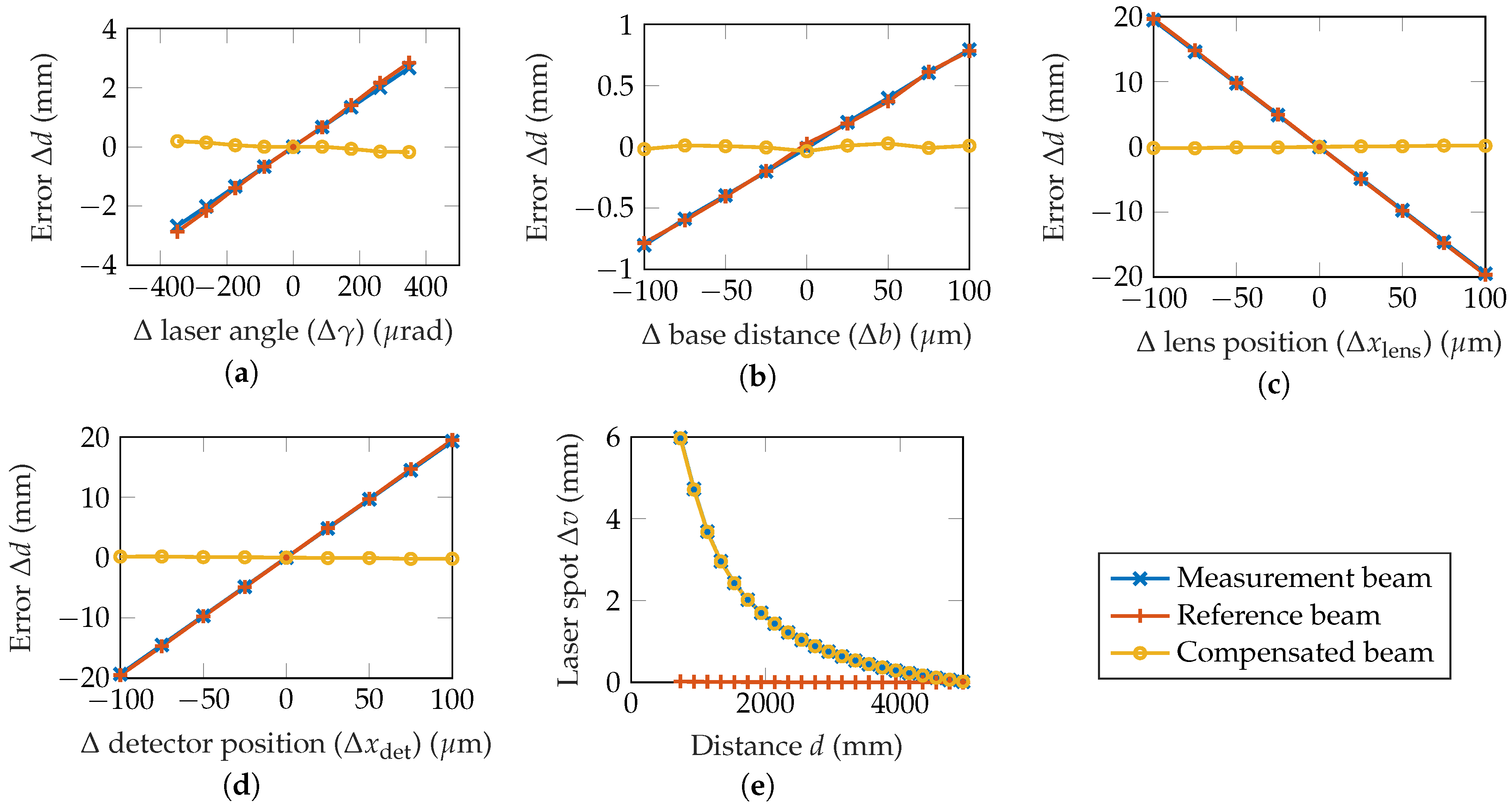
2.2. Error Model in a Laser Triangulation System

In reality, the position of the laser spot center does not only move with a change in the distance but also due to different error sources. Due to thermal drifts, mechanical instabilities, and vibrations, the direction of the laser beam can vary significantly [46], which is also referred to as laser dithering. Consequently, the laser spot moves on the measurement surface and the detector, leading to a deviation in the measured distance [15].
The laser light travels twice through the air between the measurement device and the measurement surface. In the case of air turbulences or a temperature gradient, the laser beam may be deflected, leading to an error in the calculation of the distance [5]. This can be divided into jitter and beam bending, which is the dominating error source in long-distance measurements [27].
The coherent nature of laser light in combination with the roughness of the measurement surface leads to so-called speckles in the laser spot image, resulting in a measurement error [16,47,48]. Additionally, the wide range of possible surfaces with different optical properties [17,49,50] as well as the probes position and orientation towards the measurement surface limit the accuracy of LTDs [51].
The diffusely reflected light is eventually imaged by a lens and detector. If the lens or detector shift due to temperature changes or mechanical instabilities, the laser spot moves on the detector [18], leading to an error in the measured distance. The same would apply for deviations in the optical path calibration. Ma et al. [33] showed the image translation due to self-heating of the camera to be in the order of up to two pixels in experiments.
Last but not least, there is an additional error introduced in the calculation of the center position of the laser spot. This is caused by speckles, spatial quantization, analog-to-digital quantization as well as noise on the detector, e.g., photon shot noise or dark current noise [19,52]. As the laser spot center needs to be determined with sub-pixel accuracy to achieve the desired measurement precision, this also limits the overall accuracy of an LTD.
Additionally, it has been demonstrated that distance sensors exhibit a general drift over time due to temperature fluctuations [34,53,54]. Table 1 shows an exemplary overview and impact of several parameters in a laser triangulation setup with the previously given dimensions. Hereby, the introduced distance error Δ d divided by the parameter change is denoted. The calculations are done using the paraxial approximation, assuming a perfectly thin lens without any aberrations and an infinitely small laser beam. The simulations are done using Zemax OpticStudio, taking into account the aberrations of the optical system as well as the extent of the laser beam. Consequently, there are slight differences between the values. As can be seen in Table 1, several parameters have a substantial impact on the measurement accuracy. Especially small changes in the laser angle as well as the detector and lens position can lead to significant deviations. As a temperature gradient cannot be simulated in the applied software, no value is given here. As the deviation with respect to the lens angle Δ α is a result of the aberrations of a real lens, they do not have an influence on the calculations using the paraxial approximation. Thus, no value is given here.
Deviations of the laser angle of Δγ = 0.2°, respectively 3.5 m rad , as shown in Ref. [15], would result in a measurement deviation Δ d of around 27 m m . A translation of the detector by 2 px in Ref. [33] is equivalent to a shift of 14.8 μ m (pixel pitch of 7.4 μ m ). Consequently, this would lead to a measurement deviation of around 2.9 m m . With the base distance of 130 m m and the assumption, that the components are mounted on an aluminum base (coefficient of thermal expansion of 24 µm K−1 m−1), a temperature change of 1 C would result in an increase of the base distance by 3 μ m , leading to an error in the distance measurement of around 25 μ m . Those calculations show that even small changes in the temperature or setup, in general, will lead to significant measurement errors. In order to increase the accuracy of a laser triangulation setup, these errors have to be avoided or compensated.

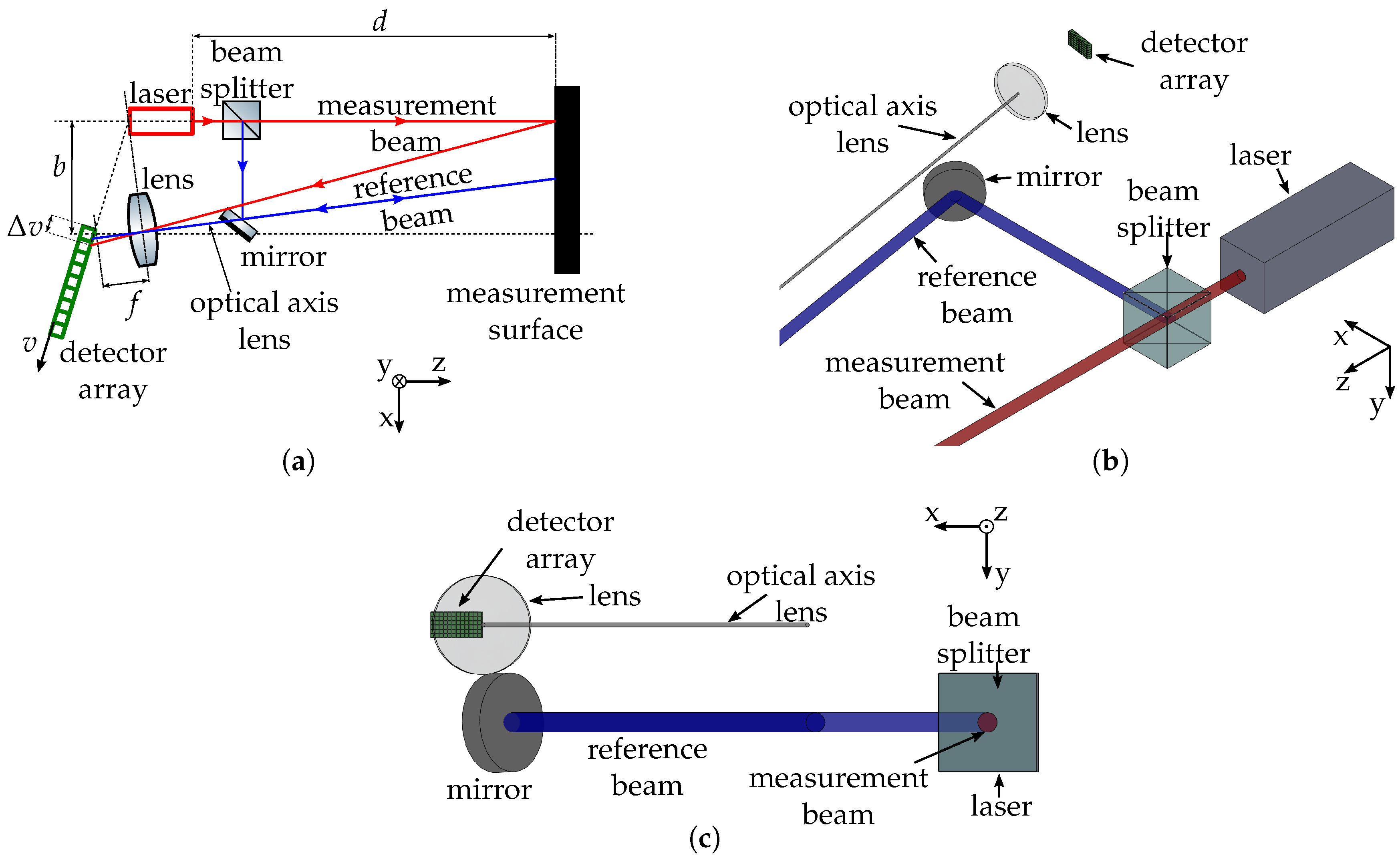
3. Optical Setup for Compensation of Measurement Errors

Several possibilities to compensate for errors have been listed in the introduction. As the previously proposed methods are either very complex or not capable of avoiding several errors simultaneously, a new compensation method is introduced here. The schematic setup can be seen in Figure 2, consisting of only an additional beam splitter and mirror. The laser beam is split up into a measurement and a reference beam, respectively. Those result in a measurement and a reference spot in the detector image, leading to the possibility to compensate for errors due to laser dithering, environmental conditions, and optomechanical shifts. Thereby, it is important that the reference beam is parallel to the optical axis of the lens. In this way, with a change of the distance d, the measurement spot center (MSC) v m e a s is changing, whereas the reference spot center (RSC) v r e f is constant. In contrast, if v m e a s is altered due to an error, v r e f changes in a similar fashion. Consequently, the deviation can be compensated by subtracting v r e f from v m e a s . The setup can either be constructed by placing the lens and detector above or below the laser in y-direction, as shown in Figure 2c. Alternatively, the beam splitter could also be tilted around the z-axis instead. Additionally, a penta prism beam splitter can be used to ensure that the reference beam is split at an angle of 90°.
The induced error Δ d of the two beams as well as of the compensated beam is given in dependence of several parameters in Figure 3a–e. The error of the compensated beam Δ d c o m p is calculated by Δ d c o m p = Δ d m e a s k · Δ d r e f , with k = 1 being the compensation factor. The results are obtained using a ray tracing simulation software. Therefor, the geometrical laser triangulation setup with its optical components is implemented in Zemax OpticStudio, and the detector image is obtained as the simulation output. Every geometrical parameter of the setup can then be varied iteratively to simulate the parameter changes reflected by the x-axis in Figure 3, e.g., the position of the lens or detector. This leads to a shift of the laser spot center in the simulated detector image, which can be transformed into a distance error Δ d using the sensitivity of the setup. This approach has the advantage that optical aberrations and the extend of the laser beam are considered here.
The errors introduced in the previous section are compensated to a good degree (Figure 3a–d), whereas a change of the measurement distance is not affected (Figure 3e).
The errors with and without compensation are summarized in Table 2. The error is reduced by up to 99%. For the laser angle and the base distance, the achieved improvement is slightly lower. As can be seen in Figure 3a,b, this is due to the different displacement of the MSC and RSC because of the different paths the beams take. Consequently, depending on what parameter needs to be compensated, the compensation factor k has to be chosen accordingly. In a real measurement setup, it is not previously known what parameters are affected by drift, so k needs to be determined experimentally. It is important that the laser output, the beam splitter and the mirror stay in a fixed relation to one another, as a change in their geometrical relation would result in a deviation of only the reference beam, leading to an error in the compensated distance measurement.
This setup has several advantages to a simple laser triangulation setup or the previously mentioned setups. First of all, it only uses two standard optical parts and does not rely on active or movable parts. Secondly, this setup is able to compensate for errors due to laser beam dithering, changes in the air refractive index as well as thermal expansions in the optomechanical setup. Thus, a less stable and more cost-effective mechanical setup, laser, and detector might be used as the drifts of those components are eliminated. Yet the setup has one disadvantage. As the two beams are not emitted in parallel, the two points typically hit the measurement surface with some distance in between them. This does not affect the measured distance, as the reference beam is parallel to the optical axis of the receiver lens, but the measurement surface needs to be wide enough so that the reference beam is diffusely reflected as well and can consequently be detected by the sensor.

4. Experimental Results

The introduced setup has then been implemented in the laboratory to verify the simulations. After a brief description of the setup, the resulting measurements are examined.

4.1. Measurement Setup

The previously introduced setup was then implemented. The fiber-coupled laser diode has a center wavelength of 660 n m and a power of 10 m W (LasersCom, LDI-660-FP-10). It is focused by an achromatic lens with a focal length of 25 m m (Throl optics GmbH). This results in a laser spot diameter of about 3.5 m m at a distance of 1 m . To achieve the desired measurement range of 800–5000 m m , the laser spot is imaged using a biconvex lens with a focal length f = 40   m m and a diameter of 31.5 m m (Linos AG), with an aperture diameter of 10 m m . The base distance b is set to 130 m m and the CMOS detector has a resolution of 3856   px × 2764   px , with a pixel pitch of 1.67 μ m (Dahua, DH-MV-A3A04MG10E). The viewing angle of the lens is set to 8°, whilst the detector is aligned according to the Scheimpflug principle. The laser is split up with a penta prism beam splitter with a relation of 50:50 (Artifex Engineering GmbH), whilst the reference beam is deflected by a Zerodur broadband dielectric mirror (Thorlabs, B111-E02). The beam splitter is tilted around the z-axis by 4° to spatially separate the two laser spots on the measurement surface.
With this setup, the desired measurement range is achieved. The theoretic relation between the laser spot center and the measurement distance can be seen in Figure 1b, as introduced before. The sensitivity of the setup is 5.1 px mm−1 at a distance of 0.8 m, 3.2 px mm−1 at a distance of 1 m, and 0.13 px mm−1 at a distance of 5 m.

4.2. Characterization of the Measurement Setup

The performance of this measurement setup is now characterized by different measurements. First of all, static measurements with a constant measurement distance d are conducted to investigate the temporal behavior of the setup due to thermal drifts. Afterward, errors are provoked to capture the efficiency of the compensation in static measurements. Finally, the measurement uncertainty in dynamic measurements over a measurement range of 910–1060 m m is determined.

4.2.1. Temporal Behavior in Static Measurements

First of all, this measurement setup is characterized in static measurements at a distance of 1 m . Thereby, the distance d is kept constant during the whole measurement. Theoretically, the laser spot center position should not move during the time. Due to the aforementioned drift of different parts, this is not true, as can be seen in a measurement of 36 h in Figure 4. Within this period, the measurement spot center changed by up to 1.12 px peak-to-peak. With the given sensitivity of 3.2 px m m , this equals a peak-to-peak distance error Δ d m e a s of 350 μ m . The correlation coefficient of the two spot centers yields a value of 0.96 , meaning that they have a strong correlation. This can also be seen in the compensated laser spot center position, which only changes within a range of 0.28 px , resulting in a distance deviation of Δ d c o m p = 88   μ m . Consequently, the static error of the long-term measurement is reduced by 75%. The drift of the signals can be explained by a slight change in the ambient temperature over time, as is indicated in Figure 4. As the correlation between the measurement laser spot center and the temperature yields a correlation coefficient of only 0.44 , the introduced error could not be compensated to such a good degree using only the temperature information.
To emphasize the compensation of both short-term and long-term drifts, Figure 5a,b show an excerpt of the highpass- and lowpass-filtered signals, respectively. For frequencies below a period duration of 15 min , it is clearly visible that the short-term variations of the signal have a high correlation of 0.96 . Therefore, short term disturbances, e.g., due to laser beam dithering, can easily be compensated. Long-term drifts, which mainly happen due to temperature changes of the setup, have a similar correlation of 0.97 , as can be seen in Figure 5b. Consequently, they can be compensated to a similar degree.
Moreover, the thermal expansion of single components was examined. A heating resistor with a value of 330 Ω was attached to the mount of the detector. To monitor the temperature change, a temperature sensor was mounted next to it. The influence of the heating up can be seen in Figure 6a. When a power of 1.7 W is dissipated in the resistor at t = 6 min for 30 s , the surrounding material is heated up by around 1 °C. As a consequence, both the measurement beam and the reference beam deviated by around 17.72 px , leading to a distance change Δ d m e a s of about 5.5 m m whereas the deviation of the compensated beam is reduced to 0.48 px or 0.15 m m . Thus, the introduced error is decreased by 97%. As this knowingly only affects the position of the detector, the compensation factor was set to 1, as has been proven as the ideal compensation factor for a sole movement of the detector in the simulations. If a compensation factor of 0.8 is applied, as in the other experiments, the deviation of the compensated beam is still reduced to Δ d c o m p = 1.06   m m , resulting in an improvement of 78%.
In additional experiments, vibrations of the measurement setup were provoked to test the ability of the setup to compensate for errors. The optical table on which the measurement setup is placed was mechanically moved. The resulting displacement of the measurement beam position and the compensated beam position is shown in Figure 6b. Whereas the measurement beam deviates by up to 5.1 px or 1.59 m m peak-to-peak, the compensated beam deviation is reduced to 0.7 px or 0.22 m m . Consequently, the deviation is reduced by 86%.

4.2.2. Dynamic Measurements

In subsequent measurements, the improvement of the compensation setup in a distance measurement is shown. The measurement surface is moved in the range of 1050–1060 m m with a step size of 5 μ m , driven by a linear translation stage with an on-axis accuracy of 5 μ m (Thorlabs, NRT150). Thereby, the position of the measurement beam is dependent on the measurement distance d, while the position of the reference beam stays relatively constant, as can be seen in Figure 7a. Consequently, the compensated beam shows the same behavior as previously introduced in Figure 3e, opening up the possibility to measure the absolute distance. A calibration polynomial of third order is calculated for both the compensated and uncompensated beam, which can be used to transfer the measured and compensated laser spot center positions into distances.
In Figure 7b, it already is visible that the uncompensated beam dithers stronger around the calibration polynomial. In a period of three days, 18 dynamic measurements were recorded. The deviation of the distance measurement Δ d can then be calculated by subtraction of the true distance d t r u e from the measured or compensated distance d m e a s or d c o m p . A comparison of the deviation between measurements using the measurement beam and the compensated beam is given in Figure 7c. As it is clearly visible, the deviation of the measurement beam is bigger compared to the deviation of the compensated beam. As a single measurement takes around 3 h , a drift of the error can be explained with a drift of the laser spot center as shown in the static measurements before. An error of 200 μ m roughly equals to a laser spot center shift by 0.6 px , which was the typical drift amplitude in the previous measurements (see Figure 4). This drift can be compensated to a good degree. Using this deviation, a root mean square error (RMSE) can be calculated, characterizing the performance of the measurement setup. Within the 18 measurements, the average RMSE is reduced from 77 μ m with the uncompensated beam to 61 μ m with the compensated beam, which equals a reduction of 22%. This improvement is not as good as it has been proven in simulations and static measurements because speckles are another major error source in laser triangulation measurements. However, the compensation setup still leads to a significant improvement in the RMSE of the distance measurement.
In the last experiment, 15 dynamic measurements in a range of 910–1060 m m with a step size of 50 μ m were conducted within five days, which equals the maximum possible translation of the stage. The resulting laser spot movement for one measurement can be seen in Figure 8a. As the reference beam is not perfectly aligned with the optical axis of the lens, the reference beam laser spot center slightly moves with the change of the distance. Consequently, the compensated beam also shows a slight deviation to the measurement beam. Within the 15 measurements, the average RMSE is reduced from 109 μ m with the measurement beam to 85 μ m with the compensated beam, which equals a reduction of 22%. The improvement is the same as it has been for the translation within 10 m m before. Yet again, the deviation of the compensated beam clearly decreased, as can be seen in Figure 8b.

5. Conclusions

In this contribution, a compensation setup for a laser triangulation device was introduced. The laser beam is split up with a simple optical setup consisting only of a beam splitter and mirror. The reference beam is directed in parallel to the optical axis of the imaging lens, resulting in a reference spot center position independent of the measurement distance. Thereby, errors resulting from laser dithering, beam bending, and optomechanical deformations can be compensated. This was shown through simulative investigations as well as measurements. As a consequence, the deviation in static measurements was reduced by 75%, while the measurement uncertainty in dynamic measurements was reduced to 85 μ m at a distance of 1 m .
A current problem of the setup is that mechanical shifts of the beam splitter or the mirror lead to an additional error that can not be compensated. As a result, those two components have to be fixed more stable, e.g., by using special temperature stabilized optical mounts made from stainless steel. With this further stabilized setup, an extensive characterization of the laser triangulation device over its complete measurement range is in the scope of subsequent investigations. During such experiments, an ideal compensation factor has to be determined. Moreover, the effects of the compensation of errors due to different surface materials, a measurement surface tilt, varying laser intensity, different types of lasers, and other error sources need to be examined, as the compensation setup could also be potentially effective for them.

Author Contributions

Conceptualization, P.K., M.H.K., K.W., M.J. and A.W.K.; methodology, P.K.; software, P.K.; validation, P.K., M.A. and L.B.; formal analysis, P.K. and L.B.; investigation, P.K. and L.B.; resources, M.J. and A.W.K.; data curation, P.K. and L.B.; writing—original draft preparation, P.K.; writing—review and editing, P.K., L.B., M.A., M.H.K., K.W., M.J. and A.W.K.; visualization, P.K.; supervision, M.J. and A.W.K.; project administration, P.K., M.J. and A.W.K.; funding acquisition, M.J. and A.W.K. All authors have read and agreed to the published version of the manuscript.

Funding

This research was funded by Bundesministerium für Wirtschaft und Energie (BMWi, ZIM, ZF4304601AB6).

Acknowledgments

The authors gratefully acknowledge the funding by the Federal Ministry for Economic Affairs and Energy of Germany (BMWi, ZIM, ZF4304601AB6) and the contributions from our project partner BLAU Optoelektronik GmbH. This work was supported by the Technical University of Munich (TUM) in the framework of the Open Access Publishing Program.

Conflicts of Interest

The authors declare no conflict of interest.

References

  1. Amann, M.C.; Bosch, T. Laser ranging: A critical review of usual techniques for distance measurement. Opt. Eng. 2001, 40, 10. [Google Scholar] [CrossRef]
  2. Blais, F. Review of 20 years of range sensor development. J. Electron. Imaging 2004, 13, 231. [Google Scholar] [CrossRef]
  3. Rivera-Castillo, J.; Flores-Fuentes, W.; Rivas-López, M.; Sergiyenko, O.; Gonzalez-Navarro, F.F.; Rodríguez-Quiñonez, J.C.; Hernández-Balbuena, D.; Lindner, L.; Básaca-Preciado, L.C. Experimental image and range scanner datasets fusion in SHM for displacement detection. Struct. Control. Health Monit. 2017, 24, e1967. [Google Scholar] [CrossRef]
  4. Guillory, J.; La Teyssendier de Serve, M.; Truong, D.; Alexandre, C.; Wallerand, J.P. Uncertainty Assessment of Optical Distance Measurements at Micrometer Level Accuracy for Long-Range Applications. IEEE Trans. Instrum. Meas. 2019, 68, 2260–2267. [Google Scholar] [CrossRef] [Green Version]
  5. Donges, A.; Noll, R. Laser Measurement Technology: Fundamentals and Applications; Springer Series in OPTICAL SCIENCES; Springer: Heidelberg, Germany, 2015; Volume 188. [Google Scholar] [CrossRef]
  6. Schuth, M.; Buerakov, W. Handbuch optische Messtechnik: Praktische Anwendungen für Entwicklung, Versuch, Fertigung und Qualitätssicherung; Hanser: München, Germany, 2017. [Google Scholar]
  7. Peiponen, K.E.; Myllylä, R.; Priezžev, A.V. Optical Measurement Techniques: Innovations for Industry and the Life Sciences; Springer Series in OPTICAL SCIENCES; Springer: Berlin, Germany, 2009; Volume 136. [Google Scholar]
  8. Ji, Z.; Leu, M.C. Design of optical triangulation devices. Opt. Laser Technol. 1989, 21, 339–341. [Google Scholar] [CrossRef]
  9. Ivanov, M.; Sergyienko, O.; Tyrsa, V.; Lindner, L.; Flores-Fuentes, W.; Rodriguez-Quinonez, J.C.; Hernandez, W.; Mercorelli, P. Influence of data clouds fusion from 3D real-time vision system on robotic group dead reckoning in unknown terrain. IEEE/CAA J. Autom. Sin. 2020, 7, 368–385. [Google Scholar] [CrossRef]
  10. Berkovic, G.; Shafir, E. Optical methods for distance and displacement measurements. Adv. Opt. Photonics 2012, 4, 441–471. [Google Scholar] [CrossRef]
  11. Wu, S.; Feng, Q.; Gao PhD, Z.; Han, Q. A Novel Laser Triangulation Sensor with Wide Dynamic Range; SAE Technical Paper Series; SAE Technical Paper; SAE International400 Commonwealth Drive: Warrendale, PA, USA, 2011. [Google Scholar] [CrossRef]
  12. Moreno-Oliva, V.I.; Román-Hernández, E.; Torres-Moreno, E.; Dorrego-Portela, J.R.; Avendaño-Alejo, M.; Campos-García, M.; Sánchez-Sánchez, S. Measurement of quality test of aerodynamic profiles in wind turbine blades using laser triangulation technique. Energy Sci. Eng. 2019, 26, 789. [Google Scholar] [CrossRef] [Green Version]
  13. Hering, E.; Martin, R. Photonik; Springer: Berlin/Heidelberg, Germany, 2006. [Google Scholar] [CrossRef]
  14. Liebe, C.C.; Coste, K. Distance Measurement Utilizing Image-Based Triangulation. IEEE Sens. J. 2013, 13, 234–244. [Google Scholar] [CrossRef]
  15. Yang, H.; Tao, W.; Zhang, Z.; Zhao, S.; Yin, X.; Zhao, H. Reduction of the Influence of Laser Beam Directional Dithering in a Laser Triangulation Displacement Probe. Sensors 2017, 17, 1126. [Google Scholar] [CrossRef] [Green Version]
  16. Ibaraki, S.; Kitagawa, Y.; Kimura, Y.; Nishikawa, S. On the limitation of dual-view triangulation in reducing the measurement error induced by the speckle noise in scanning operations. Int. J. Adv. Manuf. Technol. 2017, 88, 731–737. [Google Scholar] [CrossRef]
  17. Takushima, S.; Kawano, H.; Nakahara, H.; Kurokawa, T. On-machine multi-directional laser displacement sensor using scanning exposure method for high-precision measurement of metal-works. Precis. Eng. 2018, 51, 437–444. [Google Scholar] [CrossRef]
  18. Pedersen, D.A.K.; Liebe, C.C.; Jorgensen, J.L. Structured Light System on Mars Rover Robotic Arm Instrument. IEEE Trans. Aerosp. Electron. Syst. 2019, 55, 1612–1623. [Google Scholar] [CrossRef] [Green Version]
  19. Miao, C.; Xiao, W.; Qinghua, Y. Influence Analysis of Laser Spot Noise on the Measurement Accuracy of Laser Triangulation Method. Int. J. u- e-Serv. Sci. Technol. 2016, 9, 39–46. [Google Scholar] [CrossRef]
  20. Steele, D.S. Apparatus and Method for Optical Triangulation Measurement. FR Patent FR2487507A1, 29 January 1982. [Google Scholar]
  21. Hardin, R.A.; Liu, Y.; Long, C.; Aleksandrov, A.; Blokland, W. Active beam position stabilization of pulsed lasers for long-distance ion profile diagnostics at the Spallation Neutron Source (SNS). Opt. Express 2011, 19, 2874–2885. [Google Scholar] [CrossRef]
  22. Chang, Y.H.; Liu, C.S.; Cheng, C.C. Design and Characterisation of a Fast Steering Mirror Compensation System Based on Double Porro Prisms by a Screw-Ray Tracing Method. Sensors 2018, 18, 4046. [Google Scholar] [CrossRef] [Green Version]
  23. Yang, S.; Zhang, J.Y.; Yang, Y.Y.; Huang, J.Y.; Bai, Y.R.; Zhang, Y.; Lin, X.C. Automatic compensation of thermal drift of laser beam through thermal balancing based on different linear expansions of metals. Results Phys. 2019, 13, 102201. [Google Scholar] [CrossRef]
  24. Yong, L.; Qibo, F.; Lishuang, L.; Qingrui, Y.; Yueqiang, L. Application of optical switch in precision measurement system based on multi-collimated beams. Measurement 2015, 61, 216–220. [Google Scholar] [CrossRef]
  25. Yang, H.; Tao, W.; Yin, X.; Zhao, H. Differential correction system of laser beam directional dithering based on symmetrical beamsplitter. Opt. Rev. 2018, 25, 10–17. [Google Scholar] [CrossRef]
  26. Liu, C.S.; Jiang, S.H. A novel laser displacement sensor with improved robustness toward geometrical fluctuations of the laser beam. Meas. Sci. Technol. 2013, 24, 105101. [Google Scholar] [CrossRef]
  27. Li, J.; Wei, H.; Li, Y. Beam drift reduction by straightness measurement based on a digital optical phase conjugation. Appl. Opt. 2019, 58, 7636. [Google Scholar] [CrossRef]
  28. Dobosz, M.; Ściuba, M. Ultrasonic measurement of air temperature along the axis of a laser beam during interferometric measurement of length. Meas. Sci. Technol. 2020, 31, 045202. [Google Scholar] [CrossRef]
  29. Žbontar, K.; Mihelj, M.; Podobnik, B.; Povše, F.; Munih, M. Dynamic symmetrical pattern projection based laser triangulation sensor for precise surface position measurement of various material types. Appl. Opt. 2013, 52, 2750–2760. [Google Scholar] [CrossRef] [Green Version]
  30. Faulhaber, A.; Gronle, M.; Haberl, S.; Buchholz, T.; Haist, T.; Osten, W. Dynamically scanned spot projections with digital holograms for reduced measurement uncertainty in laser triangulation systems. In AOPC 2019: Optical Sensing and Imaging Technology; Greivenkamp, J., Ed.; SPIE: Bellingham, WA, USA, 2019; p. 167. [Google Scholar] [CrossRef]
  31. Handel, H. Analyzing the Influences of Camera Warm-Up Effects on Image Acquisition. In Computer Vision—ACCV 2007; Yagi, Y., Kang, S.B., Kweon, I.S., Zha, H., Eds.; Lecture Notes in Computer Science; Springer: Berlin, Germany, 2007; Volume 4844, pp. 258–268. [Google Scholar] [CrossRef]
  32. Handel, H. Compensation of thermal errors in vision based measurement systems using a system identification approach. In Proceedings of the 9th International Conference on Signal Processing, Denver, CO, USA, 5–7 June 2008; Yuan, B., Ed.; IEEE: Piscataway, NJ, USA, 2008; pp. 1329–1333. [Google Scholar] [CrossRef]
  33. Ma, S.; Pang, J.; Ma, Q. The systematic error in digital image correlation induced by self-heating of a digital camera. Meas. Sci. Technol. 2012, 23, 025403. [Google Scholar] [CrossRef]
  34. Li, Z.; Chen, X.; Liu, Y.; Tao, W.; Zhao, H. Temperature Compensation of Laser Triangular Displacement Sensor. In Proceedings of the 2019 Chinese Automation Congress (CAC), Hangzhou, China, 22–24 November 2019; pp. 4661–4667. [Google Scholar] [CrossRef]
  35. Flores-Fuentes, W.; Rivas-Lopez, M.; Sergiyenko, O.; Gonzalez-Navarro, F.F.; Rivera-Castillo, J.; Hernandez-Balbuena, D.; Rodríguez-Quiñonez, J.C. Combined application of Power Spectrum Centroid and Support Vector Machines for measurement improvement in Optical Scanning Systems. Signal Process. 2014, 98, 37–51. [Google Scholar] [CrossRef]
  36. So, E.W.Y.; Munaro, M.; Michieletto, S.; Antonello, M.; Menegatti, E. Real-Time 3D Model Reconstruction with a Dual-Laser Triangulation System for Assembly Line Completeness Inspection. In Intelligent Autonomous Systems 12; Lee, S., Cho, H., Yoon, K.J., Lee, J., Eds.; Advances in Intelligent Systems and Computing; Springer: Berlin/Heidelberg, Germany, 2013; Volume 194, pp. 707–716. [Google Scholar] [CrossRef] [Green Version]
  37. Selami, Y.; Tao, W.; Gao, Q.; Yang, H.; Zhao, H. A Scheme for Enhancing Precision in 3-Dimensional Positioning for Non-Contact Measurement Systems Based on Laser Triangulation. Sensors 2018, 18, 504. [Google Scholar] [CrossRef] [Green Version]
  38. Denisov, E.S.; Salakhova, A.S.; Timergalina, G.V.; Nikishin, T.P.; Azlyyyakhmatov, M.G.F. Three-Beam Triangulating Sensor. IOP Conf. Ser. Mater. Sci. Eng. 2015, 86, 012007. [Google Scholar] [CrossRef]
  39. Oh, S.; Kim, K.C.; Kim, S.H.; Kwak, Y.K. Resolution enhancement using a diffraction grating for optical triangulation displacement sensors. In Testing, Reliability, and Applications of Optoelectronic Devices; Chin, A.K., Dutta, N.K., Linden, K.J., Wang, S.C., Eds.; SPIE: Bellingham, WA, USA, 2001; p. 102. [Google Scholar] [CrossRef]
  40. Haist, T.; Gronle, M.; Bui, D.A.; Jiang, B.; Pruss, C.; Schaal, F.; Osten, W. Towards one trillion positions. In Automated Visual Inspection and Machine Vision; Beyerer, J., Puente León, F., Eds.; SPIE: Bellingham, WA, USA, 2015; p. 953004. [Google Scholar] [CrossRef]
  41. Dong, Z.; Sun, X.; Liu, W.; Yang, H. Measurement of Free-Form Curved Surfaces Using Laser Triangulation. Sensors 2018, 18, 3527. [Google Scholar] [CrossRef] [Green Version]
  42. Zhao, H.; Shi, S.; Gu, X.; Jia, G.; Xu, L. Integrated System for Auto-Registered Hyperspectral and 3D Structure Measurement at the Point Scale. Remote Sens. 2017, 9, 512. [Google Scholar] [CrossRef] [Green Version]
  43. Shi, Y.t.; Cheng, X.j. Laser Spot Center Detection Based on the Geometric Feature. In Proceedings of the International Symposium on Information Science and Engineering (ISISE), Shanghai, China, 24–26 December 2010; Chen, J., Ed.; IEEE: Piscataway, NJ, USA, 2010; pp. 322–325. [Google Scholar] [CrossRef]
  44. Song, L.; Wu, W.; Guo, J.; Li, X. Research on Sub-pixel Location of the Laser Spot Center. In Proceedings of the 2013 5th International Conference on Intelligent Human-Machine Systems and Cybernetics (IHMSC), Hangzhou, China, 26–27 August 2013; IEEE: Piscataway, NJ, USA, 2013; pp. 378–381. [Google Scholar] [CrossRef]
  45. Kienle, P.; Nallar, E.; Köhler, M.H.; Jakobi, M.; Koch, A.W. Analysis of sub-pixel laser spot detection in laser triangulation systems. In Optical Measurement Systems for Industrial Inspection XI; Lehmann, P., Osten, W., Gonçalves, A.A., Jr., Eds.; SPIE: Bellingham, WA, USA, 2019; Volume 11056, pp. 933–943. [Google Scholar] [CrossRef]
  46. Zhang, K.; Chen, H.Q.; Li, J.; Xu, J.K. An improved sub-pixel algorithm for laser spot center determination based on Zernike moments. In International Symposium on Photoelectronic Detection and Imaging 2009: Laser Sensing and Imaging; Amzajerdian, F., Gao, C.Q., Xie, T.Y., Eds.; SPIE: Bellingham, WA, USA, 2009; p. 7382. [Google Scholar] [CrossRef]
  47. Dorsch, R.G.; Häusler, G.; Herrmann, J.M. Laser triangulation: fundamental uncertainty in distance measurement. Appl. Opt. 1994, 33, 1306–1314. [Google Scholar] [CrossRef]
  48. Koch, A.W. Optische Meßtechnik an technischen Oberflächen: Praxisorientierte lasergestützte Verfahren zur Untersuchung technischer Objekte hinsichtlich Form, Oberflächenstruktur und Beschichtung; Expert-Verl.: Renningen-Malmsheim, Germany, 1998. [Google Scholar]
  49. Buzinski, M.; Levine, A.; Stevenson, W.H. Performance characteristics of range sensors utilizing optical triangulation. In Proceedings of the IEEE National Aerospace and Electronics Conference, Dayton, OH, USA, 18–22 May 1992; IEEE: Piscataway, NJ, USA, 1992; pp. 1230–1236. [Google Scholar] [CrossRef]
  50. Muralikrishnan, B.; Ren, W.; Everett, D.; Stanfield, E.; Doiron, T. Performance evaluation experiments on a laser spot triangulation probe. Measurement 2012, 45, 333–343. [Google Scholar] [CrossRef]
  51. Wu, C.; Chen, B.; Ye, C.; Yan, X. Modeling the Influence of Oil Film, Position and Orientation Parameters on the Accuracy of a Laser Triangulation Probe. Sensors 2019, 19, 1844. [Google Scholar] [CrossRef] [Green Version]
  52. Haist, T.; Dong, S.; Arnold, T.; Gronle, M.; Osten, W. Multi-image position detection. Opt. Express 2014, 22, 14450–14463. [Google Scholar] [CrossRef] [PubMed]
  53. Nan, Z.; Feng, Y.U.; Zhao, H.; Tao, W. Research on laser source drift with temperature of laser triangular displacement sensor. In Proceedings of the Ninth International Symposium on Precision Mechanical Measurements, Chongqing, China, 18–21 October 2019; Yu, L., Ed.; SPIE: Bellingham, WA, USA, 2019. [Google Scholar] [CrossRef]
  54. Liu, L.; Yang, Y.; Yang, B. Non-contact and high-precision displacement measurement based on tunnel magnetoresistance. Meas. Sci. Technol. 2020, 31, 065102. [Google Scholar] [CrossRef]
Figure 1. (a) Schematic of a laser triangulation setup consisting of a laser, a lens and a detector array in Scheimpflug condition. (b) Relation between the laser spot center v L and the distance d according to Equation (1). Sensitivity of the setup, defined by the shift of the laser spot center over the corresponding distance change. The detector is shifted in v-direction such that a maximum measurement distance of approximately 5000 m m is achieved ( v o f f s e t 1   m m ).
Sensors 20 04949 g001
Figure 2. Schematic of a setup able to compensate for errors due to laser beam dithering, air refractive gradients and optomechanical thermal effects. (a) Schematic top view. (b) Isometric CAD view. (c) Frontal CAD view.
Sensors 20 04949 g002
Figure 3. Simulated distance errors Δ d of the measurement beam, the reference beam as well as the compensated beam ( Δ d m e a s Δ d r e f ) in dependence of a deviation of (a) the laser beam angle, (b) base distance Δ b , (c) lens position Δ x , (d) detector position Δ x , and (e) measurement distance d.
Sensors 20 04949 g003
Figure 4. Measurement showing the compensation of drift effects. The measurement beam shows a stronger deviation than the compensated beam. A slight correlation of the measurement beam with the room temperature is visible.
Sensors 20 04949 g004
Figure 5. (a) Highpass-filtered data showing the compensation of short-term drift effects. A minimum-order filter with a passband frequency of 1.11 m Hz , steepness of 0.85 and stopband attenuation of 60 dB was applied. (b) Lowpass-filtered data showing the compensation of long-term drift effects. A moving average filter with a window length of 1 h was applied.
Sensors 20 04949 g005
Figure 6. (a) A heating resistor at the camera mount was turned on after 6 min for a duration of 30 s. This results in a shift of the MSC due to the thermal expansion, whereas the compensated beam position is not affected. (b) Due to mechanical vibrations at the optical table the measurement beam position shows a movement, whilst the impact is strongly reduced in the compensated beam position.
Sensors 20 04949 g006
Figure 7. (a) Dynamic measurement over the range of 10 m m . (b) Close-up on part of the measurement, highlighting the improvement using the compensated beam. (c) Measurement deviation of the compensated and uncompensated beam.
Sensors 20 04949 g007
Figure 8. Dynamic measurement in a range of 150 m m . (a) Comparison of the measurement, reference and compensated beam position. (b) Measurement deviation for the measurement and compensated beam.
Sensors 20 04949 g008
Table 1. Relationship between distance error Δ d and parameter changes at a measurement distance of d = 1   m . For example with a change of the laser angle by Δ γ = 1   μ rad , the calculated distance changes by Δ d = 7.7   μ m .
CategoryParameterCalculationSimulation
Laser ditheringLaser angle Δ γ 7.7   μ m / μ rad 7.6   μ m / μ rad
Beam bendingTemperature gradient 3.6   μ m /( K / m )- - -
Optomechanical SetupBase distance Δ b 7.8   μ m / μ m 8.0   μ m / μ m
Lens position Δ x l e n s 195 μ m / μ m 195 μ m / μ m
Lens position Δ z l e n s 25.8   μ m / μ m 23.4   μ m / μ m
Lens angle Δ α - - - 0.7   μ m / μ rad
Detector position Δ x d e t 193 μ m / μ m 193 μ m / μ m
Detector position Δ z d e t 24.10   μ m / μ m 22.3   μ m / μ m
Table 2. Relationship between distance error Δ d in dependence of parameter changes at a measurement distance of d = 1   m .
ParameterUncompensatedCompensatedReduction by
Δ laser angle ( Δ γ ) 7.6   μ m / μ rad 0.53   μ m / μ rad 93.1%
Δ base distance ( Δ b ) 8 μ m / μ m 0.32   μ m / μ rad 96.0%
Δ lens position ( Δ x l e n s ) 195 μ m / μ m 2 μ m / μ m 99.0%
Δ detector position ( Δ x d e t ) 193 μ m / μ m 2 μ m / μ m 99.0%

