Application of Least Squares with Conditional Equations Method for Railway Track Inventory Using GNSS Observations

Abstract

Satellite geodetic networks are commonly used in surveying tasks, but they can also be used in mobile surveys. Mobile satellite surveys can be used for trackage inventory, diagnostics and design. The combination of modern technological solutions with the adaptation of research methods known in other fields of science offers an opportunity to acquire highly accurate solutions for railway track inventory. This article presents the effects of work carried out using a mobile surveying platform on which Global Navigation Satellite System (GNSS) receivers were mounted. The satellite observations (surveys) obtained were aligned using one of the methods known from classical land surveying. The records obtained during the surveying campaign on a 246th km railway track section were subjected to alignment. This article provides a description of the surveying campaign necessary to obtain measurement data and a theoretical description of the method employed to align observation results as well as their visualisation.

1. Introduction

The development of modern rail transport is associated, inter alia, with increasing train speed. This causes specific problems related to railway traffic control, as described, for example, in [1], or with designing fast railway stops as described, for example, in [2]. An increase in train speed requires, primarily, that a high level of rail transport safety should be ensured, which is not possible without well-developed railway infrastructure constructed with the utmost care. Therefore, there is a need to monitor trackages, both at the construction stage and during operation [3]. The assessment of railway track is important not only for assurance of a high level of rail transport, but it is also necessary for providing high-quality transport services, as described in [4]. For the assessment of railway track geometry, track gauges and measuring trolleys are used, whose application examples can be found in the literature on the subject, e.g., in [5] or in [6]. However, in the last twenty years, Global Navigation Satellite Systems (GNSS) have become the very basic precise instrument used worldwide. GNSS and the relative instrumentation are under systematic development and constantly increase the application possibilities, which has resulted in their widespread use despite the emerging hazards in operation [7,8]. The main application of GNSS is in geodesy but they are more often used to determine the position of objects in motion [9,10] in the process of directly ensuring a high level of safety of maritime navigation, e.g., [11], or they support the process of modelling the surrounding reality in the computer environment, e.g., [12]. It has become clear that there are possibilities for the application of GNSS in railway transport, e.g., for monitoring railway infrastructure.

The proposal for the performance of mobile surveys involving the geodetic inventory of railway tracks using Global Navigation Satellite Systems (GNSS) in railway engineering appeared for the first time in Poland [13]. The proposals for the new use of positioning techniques were verified during the initial experimental tests while taking an inventory of the railway route between Koscierzyna and Kartuzy in Poland [14], when four GNSS receivers were used as well as the ASG-EUPOS Polish active satellite GNSS surveying network [15]. The study results confirmed the extensive application possibilities for the method and drew attention to its limitations due to signal availability in a built-up area. Launching new GNSS systems (Galileo, Beidou) and creating multiconstellation GNSS surveying networks [16] while increasing the accuracy of the existing ones (Navstar GPS/Glonass) allowed the authors to develop this method [17]. In the period 2009–2017, while developing the method of mobile satellite surveys, research was carried out in two main directions, i.e., the land surveying method associated with increasing accuracy and availability of measurements ([18,19,20]) and the construction method aimed at developing new design and operational methods [21,22,23,24,25]. At other research centres, analogous studies were also undertaken to integrate tacheometric and GNSS surveys [26], with measurement support through the application of inertial navigation systems (INS) [27,28] or the application of mobile laser scanners [29,30]. In addition, studies were conducted to apply multisensor methods [31,32,33,34,35,36].

A very important aspect is increasing the accuracy of determining the position of designated vehicles using GNSS. To this end, it is worth applying techniques and methods for aligning observation results used in land surveying. The literature provides examples of the application of land surveying alignment methods in rail transport, e.g., [37] which described the application of the conditional observation alignment method or referred to the estimation of the accuracies obtained during traditional static surveys [38]. In [38] the authors describe the use of automated measurement systems based on trolleys for track surveying supported with automatic tacheometric surveys. Moreover, there are examples of the application of geodetic alignment methods in maritime transport, e.g., [39,40]. These articles present the results of work related to the adaptation of a surveying method for aligning observation results, known as the method of least squares with conditional equations in mobile surveys. The alignment process was checked using the records of GNSS signals during the mobile surveying campaign conducted in July 2019 on a 246-km-long section between Tczew–Chojnice–Brusy–Chojnice–Tczew located in northern Poland.

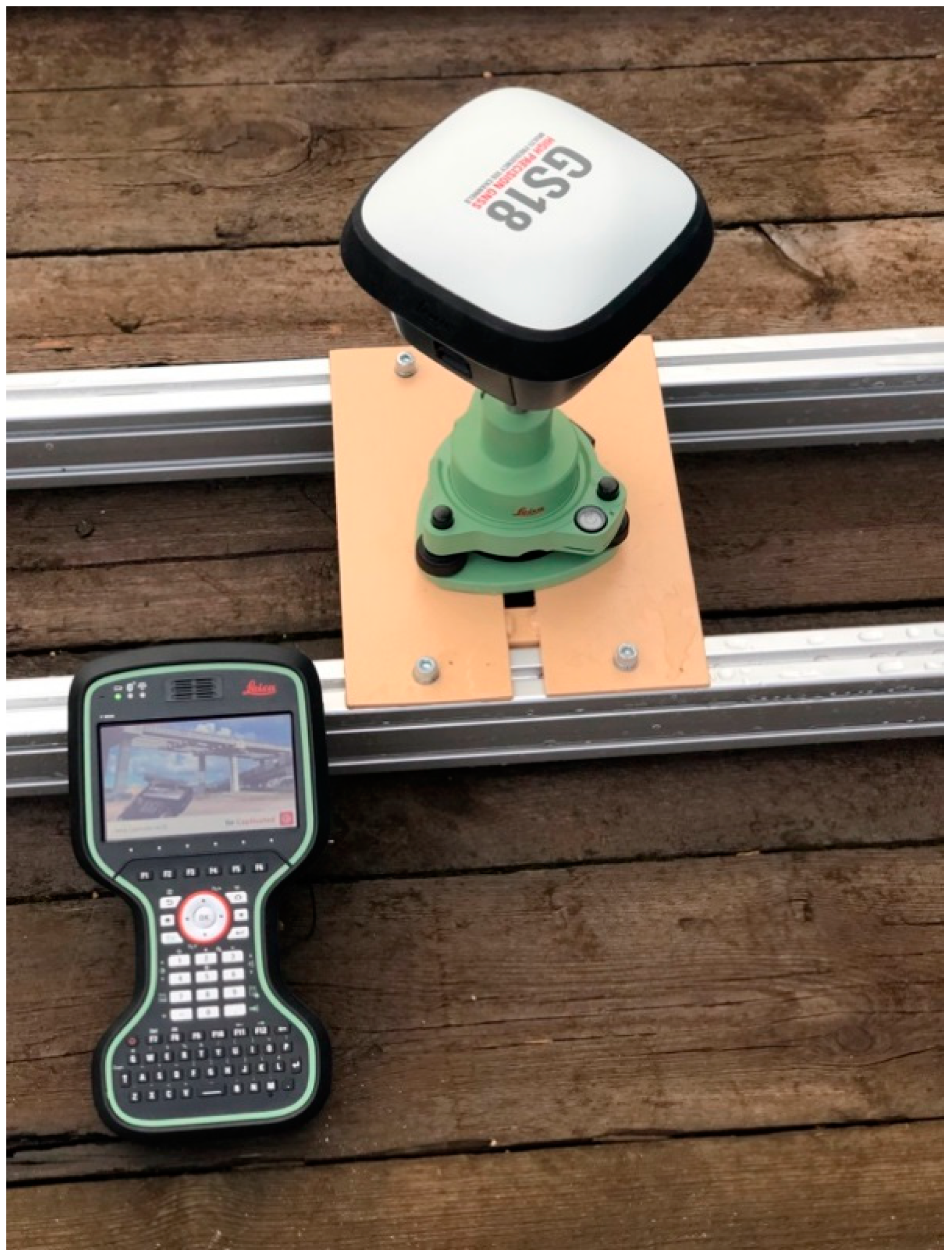
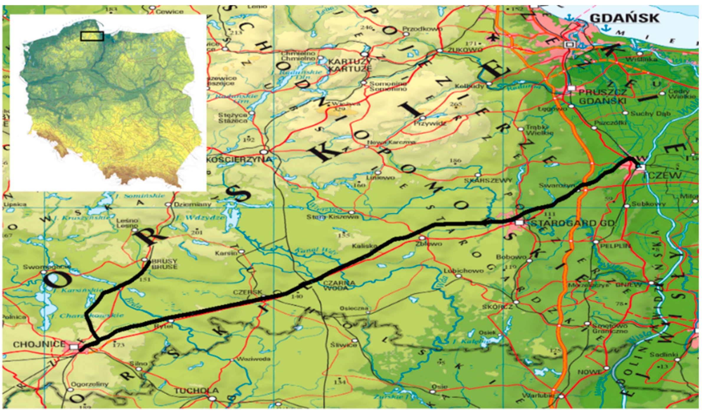
2. Mobile Surveying Platform

To obtain GNSS surveying data that enable an assessment of the railway track geometry during dynamic surveys (in motion), it was necessary to design and build a mobile surveying platform (MSP). The MSP was conceptualised and developed as part of a research project implemented by the Gdansk University of Technology and Gdynia Maritime University. The mobile surveying platform comprises a railway car (Figure 1) on which nine mounted guides have been installed to mount measuring instruments (GNSS receivers, INS systems, a mobile laser scanner and visual systems), a power generator and a workstation recording data from the installed sensors.

On the surveying platform prepared in this way, any given number of measuring instruments can be installed. During the surveys, the car was connected to a DH-350.11 hydraulic handcar. In this configuration, the test team can configure recorders depending on the type of research for which it is to be used.

3. Theoretical Basis of the Method of Least Squares with Conditional Equations

In geodetic surveys, there are alignment tasks in which the parameters of the system of observation equations must satisfy additional conditions [41]. In geodetic networks, these conditions may concern the coordinates of certain points being part of a particular network. Such a case occurs when the distance between points is determined with high accuracy, or the conditions between the coordinates result from the geometric structure of the network. Such a case is found in the research problem under consideration, where the position of antennas on the surveying platform are determined from satellite observations as well as from tacheometric surveys conducted prior to the measurement session using satellite measurement techniques. The distances between GNSS receiver antennas were precisely measured prior to commencing dynamic surveys. The geodetic inventory of GNSS antennas was carried out using an electronic total station and the values obtained were adopted as observations determined with high accuracy, which justifies the assumption that they are relatively error-free. Therefore, it follows that the parameters of the observation system (coordinates of GNSS antennas’ measuring points on the surveying platform) must satisfy additional conditions, i.e., the distances between GNSS antennas on the MSP. For the cumulative processing of the obtained observations, the Method of Least Squares with conditional equations (LSce) can then be applied. The theory behind the method was discussed in detail inter alia in [42,43]. Its further developments and applications to prepare geodetic observations are discussed inter alia in [41], [44,45]. It should also be noted that conditional equations have also been used in other estimation methods, e.g., in M_split estimation [46]. The initial tests of the application of LSce to estimate the GNSS receiver antennas’ coordinates on surveying platforms were carried out over the test section of tram tracks in the urban agglomeration of Gdansk [47].

Below are the main assumptions and the ways to apply LSce in the context of the surveying platform and the associated observation systems considered in this study.

Let us assume that the coordinates of antennas $(x_i,y_i)$, $i=1,2,\cdots ,s$, on the surveying platform, are contained in the vector $X={[x_1,y_1,\dots ,x_s,y_s]}^T={[X_1,X_2,\dots ,X_r]}^T$ (s—the number of antennas, r—the number of unknown coordinates). Following the previous assumptions about the adopted measurement structure, these quantities must satisfy the following system of conditional equations:

$$\begin{array}{l}{\mathrm{\Psi }}_1\left(X_1,X_2,\dots ,X_r\right)=0\\ {\mathrm{\Psi }}_2\left(X_1,X_2,\dots ,X_r\right)=0\\ ⋮\\ {\mathrm{\Psi }}_w\left(X_1,X_2,\dots ,X_r\right)=0\end{array}\}\iff \mathrm{\Psi }\left(X\right)=0$$

(1)

For example, if we assume that $(x_i,y_i)$ $(x_j,y_j)$ are the coordinates of two antennas between which the distance $d_{ij}$ was measured with high accuracy, then ${[{(x_j-x_i)}^2+{(y_j-y_i)}^2]}^{1/2}-d_{ij}=0$. Moreover, in accordance with the general principles of determining geodetic network coordinates, the vector $X$ is determined based on GNSS satellite observations which enable the formulation of the following system of observation equations:

$$\begin{array}{l}{y}_1+v_1=F_1\left(X_1,X_2,\dots ,X_r\right)\\ y_2+v_2=F_2\left(X_1,X_2,\dots ,X_r\right)\\ ⋮\\ y_n+v_n=F_n\left(X_1,X_2,\dots ,X_r\right)\end{array}\}\iff y+v=F\left(X\right)$$

(2)

where $y={[y_1,y_2\cdots ,y_n]}^T$ is the observation vector. Using $v={[v_1,v_2\cdots ,v_n]}^T$, the vector of random observation errors with the covariance matrix $C_v={\sigma }_0^{2}Q={\sigma }_0^2{P}_{}^{-1}$ and the vector of expected values $E(v)=0$ ($Q$—known cofactor matrix, $P$—weight matrix, ${\sigma }_0^2$—unknown variance coefficient). When we assume that the approximate coordinates $X^0={[X_1^0,\dots ,X_r^0]}^T$ of GNSS receiver antennas are known, then the equation $y+v=F\left(X\right)$ can be replaced with a linear observation equation with the following form:

$$v=F\left(X\right)-y=F\left(X^0+dX\right)-y={\frac{\partial F\left(X\right)}{\partial X}|}_{X=X^0}dX+F\left(X^0\right)-y=AdX+l$$

(3)

The quantity $dX$ is the vector of unknown coordinate increments, such that $X=X^0+dX$. The matrix

$$A={\frac{\partial F\left(X\right)}{\partial X}|}_{X=X^0}={\left[\begin{array}{cccc}\frac{\partial F_1\left(X\right)}{\partial X_1}& \frac{\partial F_1\left(X\right)}{\partial X_2}& \cdots & \frac{\partial F_1\left(X\right)}{\partial X_r}\\ \frac{\partial F_2\left(X\right)}{\partial X_1}& \frac{\partial F_2\left(X\right)}{\partial X_2}& \cdots & \frac{\partial F_2\left(X\right)}{\partial X_r}\\ \cdots & \cdots & \cdots & \cdots \\ \frac{\partial F_n\left(X\right)}{\partial X_1}& \frac{\partial F_n\left(X\right)}{\partial X_2}& \cdots & \frac{\partial F_n\left(X\right)}{\partial X_r}\end{array}\right]}_{X=X^0}$$

is the design of the system of linear equations, while

$$l=F\left(X^0\right)-y={\left[F_1\left(X^0\right)-y_1,F_2\left(X^0\right)-y_2,\cdots ,F_n\left(X^0\right)-y_n\right]}^T$$

is the absolute term vector. Let us also assume that the matrix $A$ is a column full rank, i.e., $rank(A)=r$. Considering that $X=X^0+dX$, the system of observation equations (1) can also be similarly brought to the linear form. After developing the function $\Psi \left(X\right)$ to the form

$$\mathrm{\Psi }\left(X\right)=\mathrm{\Psi }\left(X^0+dX\right)=\mathrm{\Psi }\left(X^0\right)+{\frac{\partial \mathrm{\Psi }\left(X\right)}{\partial X}|}_{X=X^0}dX=\mathrm{\Psi }\left(X^0\right)+BdX$$

(4)

the following linear conditional equation is obtained:

$$BdX+\Delta =0$$

(5)

where:

$$B={\frac{\partial \mathrm{\Psi }\left(X\right)}{\partial X}|}_{X=X^0}={\left[\begin{array}{cccc}\frac{\partial {\mathrm{\Psi }}_1\left(X\right)}{\partial X_1}& \frac{\partial {\mathrm{\Psi }}_1\left(X\right)}{\partial X_2}& \cdots & \frac{\partial {\mathrm{\Psi }}_1\left(X\right)}{\partial X_r}\\ \frac{\partial {\mathrm{\Psi }}_2\left(X\right)}{\partial X_1}& \frac{\partial {\mathrm{\Psi }}_2\left(X\right)}{\partial X_2}& \cdots & \frac{\partial {\mathrm{\Psi }}_2\left(X\right)}{\partial X_r}\\ \cdots & \cdots & \cdots & \cdots \\ \frac{\partial {\mathrm{\Psi }}_w\left(X\right)}{\partial X_1}& \frac{\partial {\mathrm{\Psi }}_w\left(X\right)}{\partial X_2}& \cdots & \frac{\partial {\mathrm{\Psi }}_w\left(X\right)}{\partial X_r}\end{array}\right]}_{X=X^0},$$

$$\Delta =\mathrm{\Psi }\left(X^0\right)={\left[{\mathrm{\Psi }}_1\left(X^0\right),{\mathrm{\Psi }}_2\left(X^0\right),\cdots ,{\mathrm{\Psi }}_w\left(X^0\right)\right]}^T.$$

Taking into account the conditions binding the parameters being determined, and the application of the objective function of the least-squares method, it leads to the optimisation of the problem with the following form (e.g., [38]):

$$\begin{array}{l}AdX+l=v\\ BdX+\Delta =0\\ C_v={\sigma }_0^2{P}_{}^{-1}\\ \phi (dX)=v^{T}Pv=\min \end{array}\}$$

(6)

In order to exactly solve this problem, it is necessary to replace the original objective function $\phi (dX)=v^{T}Pv$ with the Lagrange function with the following form (e.g., [39])

$${\phi }_L(dX)=\phi (dX)-2{\kappa }^T(BdX+\Delta )=v^{T}Pv-2{\kappa }^T(BdX+\Delta )$$

(7)

where $\kappa$ is the Lagrange’s unknown multiplier vector. The optimisation problem $\min {\phi }_L(dX)={\phi }_L(d\widehat{X})$ solves such quantities for which the following sufficient conditions are satisfied:

$${\frac{\partial {\phi }_L(dX)}{\partial dX}|}_{\widehat{\kappa },d\widehat{X}}={\frac{\partial {\phi }_L(dX)}{\partial v}\frac{\partial v}{\partial dX}|}_{\widehat{\kappa },d\widehat{X}}=2{\widehat{v}}^{T}PA-2{\widehat{\kappa }}^{T}B=0$$

(8)

$${\frac{\partial {\phi }_L(dX)}{\partial \widehat{\kappa }}|}_{\widehat{\kappa },d\widehat{X}}=Bd\widehat{X}+\Delta =0$$

(9)

Moreover, in the issue under consideration, the necessary condition involving the positive-definite of the second derivative ${\partial }^2{\phi }_L(dX)/\partial v\partial v^T=2P$ should be satisfied here. It follows from Equation (8) that

$$AP\widehat{v}-B^T\widehat{\kappa }=0\iff A^{T}PAd\widehat{X}+A^{T}Pl-B^T\widehat{\kappa }=0$$

(10)

If $rank(A^{T}PA)=rank(A)=r$, then the solution to Equation (10) is vector

$$d\widehat{X}=-{(A^{T}PA)}^{-1}(A^{T}Pl-B^T\widehat{\kappa })$$

(11)

The correlate vector must satisfy the condition (9). By substituting vector $d\widehat{X}$ described with the dependence (11) to the equation $Bd\widehat{X}+\Delta =0$, the following is obtained:

$$\widehat{\kappa }=-{\left[B{\left(A^{T}PA\right)}^{-1}{B}^T\right]}^{-1}\left[\Delta -B{\left(A^{T}PA\right)}^{-1}{A}^{T}PL\right]$$

(12)

In practice, task (6) can also be solved in a different way that is simpler from the numerical perspective. To this end, the conditional equation $BdX+\Delta =0$ should be replaced with the equivalent observation equation:

$$BdX+\Delta =v_{\ast }$$

(13)

Since it is required that $v_{\ast }=0$, therefore the vector of fictitious observation errors $v_{\ast }$ should be assigned such a covariance matrix $C_{v_{\ast }}={\sigma }_0^2{P}_{\ast }^{-1}$ so that also fictitious corrections ${\widehat{v}}_{\ast }$ meet the condition ${\widehat{v}}_{\ast }=0$ (within the calculation precision limits). Thus, task (6) is replaced with the optimisation problem, classical for the LS-method, with the following form:

$$\begin{array}{l}\begin{array}{c}AdX+l=v\\ \begin{array}{l}BdX+\Delta =v_{\ast }\\ C_v={\sigma }_0^2{P}_{}^{-1}\\ C_{v_{\ast }}={\sigma }_0^2{P}_{\ast }^{-1}\end{array}\end{array}\\ \phi (dX)=v^{T}Pv+v_{*}^T{P}_{\ast }{v}_{\ast }=\min \end{array}\}\iff \{\begin{array}{l}\stackrel{⌢}{A}dX+\stackrel{⌢}{l}=\stackrel{⌢}{v}\\ {\stackrel{⌢}{C}}_v={\sigma }_0^2{\stackrel{⌢}{P}}_{}^{-1}\\ \phi (dX)={\stackrel{⌢}{v}}^T\stackrel{⌢}{P}\stackrel{⌢}{v}=\min \end{array}$$

(14)

where:

$$\stackrel{⌢}{A}=\left[\begin{array}{c}A\\ B\end{array}\right],\stackrel{⌢}{l}=\left[\begin{array}{c}l\\ \Delta \end{array}\right],\stackrel{⌢}{v}=\left[\begin{array}{l}v\hfill \\ v_{\ast }\hfill \end{array}\right].$$

Vector $\stackrel{⌢}{v}$ is the total vector of observation errors with the covariance matrix of:

$$\stackrel{⌢}{C}=\left[\begin{array}{cc}{C}_v={\sigma }_0^2{P}_{}^{-1}& 0\\ 0& C_{v_{\ast }}={\sigma }_0^2{P}_{\ast }^{-1}\end{array}\right]={\sigma }_0^2\left[\begin{array}{cc}{P}_{}^{-1}& 0\\ 0& P_{\ast }^{-1}\end{array}\right]={\sigma }_0^2{\stackrel{⌢}{P}}^{-1}$$

(15)

where $\stackrel{⌢}{P}=\mathrm{diag}(P,P_{*})$ is the total weight matrix (${\sigma }_0^2$—variance coefficient common for both components of the model (15). The solution to task (14) is the increment estimator $d\widehat{X}$ with the following form:

$$d\widehat{X}=-{({\stackrel{⌢}{A}}^T\stackrel{⌢}{P}\stackrel{⌢}{A})}^{-1}{\stackrel{⌢}{A}}^T\stackrel{⌢}{P}\stackrel{⌢}{l}$$

(16)

where: ${\stackrel{⌢}{A}}^T\stackrel{⌢}{P}\stackrel{⌢}{A}=A^{T}PA+B^T{P}_{\ast }B$, ${\stackrel{⌢}{A}}^T\stackrel{⌢}{P}\stackrel{⌢}{l}=A^{T}Pl+B^T{P}_{\ast }\Delta$. By determining the covariance matrix for this estimator, the following is obtained:

$$C_{d\widehat{X}}={\widehat{\sigma }}_0^2{({\stackrel{⌢}{A}}^T\stackrel{⌢}{P}\stackrel{⌢}{A})}^{-1}$$

(17)

where:

$${\widehat{\sigma }}_0^2=\frac{{\widehat{\stackrel{⌢}{v}}}^T\stackrel{⌢}{P}\widehat{\stackrel{⌢}{v}}}{n+w-r}$$

(18)

is an estimator of variance coefficient ${\sigma }_0^2$. The vector $\widehat{\stackrel{⌢}{v}}={[{\widehat{v}}_{}^T,{\widehat{v}}_{\ast }^T]}^T$ is a total correction vector determined from the following dependence:

$$\widehat{\stackrel{⌢}{v}}=\stackrel{⌢}{A}d\widehat{X}+\stackrel{⌢}{l}$$

(19)

The estimator of the GNSS receiver antennas’ coordinates is the vector:

$$\widehat{X}=X^0+d\widehat{X}$$

(20)

with the covariance matrix $C_{\widehat{X}}=C_{d\widehat{X}}$ It should be noted that the diagonal elements of this matrix are the squares of mean errors of the determined estimators, i.e., $m_{{\widehat{X}}_i}^2={[C_{\widehat{X}}]}_{ii}$.

Considering both presented solutions, the exact one represented by the alignment task (6) with the estimator (11), and the equivalent one represented by the alignment task (14) with the estimator (16) yield the same solutions. Therefore, the equivalent solution that was used in the problem described in this article is more often applied in technical applications.

4. Practical Applications of GNSS in Railway Surveys and Alignment Results

On 16–17 July 2019, on a route between Tczew–Chojnice–Brusy–Chojnice–Tczew, located in northern Poland, a study was conducted using six Leica GS-18 GNSS receivers (Figure 2).

Selected technical data of the receiver are provided in the

Table 1. Selected parameters of a LEICA GS 18T receiver.

Parameter	Value
Signals Tracked	GPS (L1, L2, L2C, L5), Glonass (L1, L2, L2C, L32), BeiDou (B1, B2, B32), Galileo (E1, E5a, E5b, Alt-BOC, E62), QZSS (L1, L2C, L5, L62), NavIC L53, SBAS (WAAS, EGNOS, MSAS, GAGAN), Band L
Initialisation Time	Normally 4 s
Rtk Accuracy	A single baseline: Hz 8 mm + 1 ppm/V 15 mm + 1 ppm Network RTK: Hz 8 mm + 0.5 ppm/V 15 mm + 0.5 ppm
Postprocessing Accuracy	Static mode (phase), long-term observations: Hz 3 mm + 0.1 ppm/V 3.5 mm + 0.4 ppm, Static and fast static mode (phase): Hz 3 mm + 0.5 ppm/V 5 mm + 0.5 ppm
Weight	1.20 kg/3.50 kg—a standard configuration of an RTK receiver on a pole
Dimensions	173 mm × 173 mm × 108 mm
Position Measurement	5 Hz/20 Hz

.

On the day preceding the proper measurements, surveying devices and instruments were mounted on a railway car (Figure 3).

To precisely determine the distance between the receiver antennas axes, tacheometric surveys were then conducted using a LEICA TS 1103 total station. The measured distances are provided in Figure 4.

Six GNSS receivers were used in the study. Furthermore, 507,251 coordinate surveys were obtained for each receiver from the conducted observations, after rejecting incomplete observations. The data obtained were aligned using the Method of Least Squares with conditional equations.

The observation results were aligned in the flat rectangular coordinate system PL-2000. The system was developed based on the mathematically unique alignment of points on the reference spheroid GRS80 with the corresponding points on the plane, in accordance with the Gauss-Krüger projection theory, and is valid in the territory of the Republic of Poland [48].

Because of the large number of data, the alignment results for only one measurement epoch (marked as 20190717_104340150), conducted in postprocessing, are presented below. The following input data were obtained from satellite observations (

Table 2. Coordinates of GNSS receiver antennas along with the errors of their determination, obtained from satellite observations.

GNSS Receiver	x	y	m
GNSS #1	5967572.5583	6505456.2272	0.0669
GNSS #2	5967571.9058	6505456.6093	0.2609
GNSS #3	5967571.2635	6505456.9836	0.0966
GNSS #4	5967576.0405	6505462.2802	0.0046
GNSS #5	5967575.3857	6505462.6552	0.0285
GNSS #6	5967574.7377	6505463.0309	0.0404

):

• coordinates of GNSS antennas on the MSP,
• errors in determining the GNSS antenna position coordinates.

The position of antennas on the surveying platform is shown in the Figure 5.

Moreover, for further calculations, the measured distances between antennas (Figure 4) as well as errors of their determination: $m_{1-3}=0.0031$, $m_{1-4}=0.0033$, $m_{2-5}=0.0034$, $m_{3-6}=0.0035$, $m_{4-6}=0.0030$, resulting from the total station instrumental errors, were used. In the calculations, the measured distances to three reference stations being part of the SmartNet network [49] were used. The coordinates of the station exposures are provided in the

Table 3. Coordinates of the SmartNet network reference stations.

Station Name	x	y
Starogard Gdański	5981664.913	6532343.251
Konarzyny	5965574.243	6460849.453
Czersk	5962606.324	6498027.094

.

The measured data allowed the system of equations comprising 18 observation equations (2) and 5 conditional equations (1) to be recorded. The solution to the alignment task (14) for the data provided above was possible on the assumption that the matrices $\stackrel{⌢}{A}$ and $\stackrel{⌢}{l}$ have the following forms:

$$\stackrel{⌢}{A}=\left[\begin{array}{cccccccccccc}-0.46423& -0.88571& 0& 0& 0& 0& 0& 0& 0& 0& 0& 0\\ 0& 0& -0.46425& -0.88570& 0& 0& 0& 0& 0& 0& 0& 0\\ 0& 0& 0& 0& -0.46427& -0.88569& 0& 0& 0& 0& 0& 0\\ 0& 0& 0& 0& 0& 0& -0.46422& -0.88572& 0& 0& 0& 0\\ 0& 0& 0& 0& 0& 0& 0& 0& -0.46425& -0.88571& 0& 0\\ 0& 0& 0& 0& 0& 0& 0& 0& 0& 0& -0.46427& -0.88570\\ 0.04475& 0.99900& 0& 0& 0& 0& 0& 0& 0& 0& 0& 0\\ 0& 0& 0.04474& 0.99900& 0& 0& 0& 0& 0& 0& 0& 0\\ 0& 0& 0& 0& 0.04472& 0.99900& 0& 0& 0& 0& 0& 0\\ 0& 0& 0& 0& 0& 0& 0.04483& 0.99899& 0& 0& 0& 0\\ 0& 0& 0& 0& 0& 0& 0& 0& 0.04481& 0.99900& 0& 0\\ 0& 0& 0& 0& 0& 0& 0& 0& 0& 0& 0.04480& 0.99900\\ 0.55574& 0.83135& 0& 0& 0& 0& 0& 0& 0& 0& 0& 0\\ 0& 0& 0.55567& 0.8314& 0& 0& 0& 0& 0& 0& 0& 0\\ 0& 0& 0& 0& 0.55560& 0.83145& 0& 0& 0& 0& 0& 0\\ 0& 0& 0& 0& 0& 0& 0.55570& 0.83138& 0& 0& 0& 0\\ 0& 0& 0& 0& 0& 0& 0& 0& 0.55563& 0.83143& 0& 0\\ 0& 0& 0& 0& 0& 0& 0& 0& 0& 0& 0.55556& 0.83148\\ 0.86346& -0.50442& 0& 0& -0.86346& 0.50442& 0& 0& 0& 0& 0& 0\\ 0& 0& 0& 0& 0& 0& 0.86645& 0.49927& 0& 0& -0.86645& 0.49927\\ -0.49866& -0.86680& 0& 0& 0& 0& 0.49866& 0.86680& 0& 0& 0& 0\\ 0& 0& -0.49885& -0.86669& 0& 0& 0& 0& 0.49885& 0.86669& 0& 0\\ 0& 0& 0& 0& -0.49815& -0.86709& 0& 0& 0& 0& 0.49815& 0.86709\end{array}\right],\stackrel{⌢}{l}=\left[\begin{array}{c}0\\ 0\\ 0\\ 0\\ 0\\ 0\\ 0\\ 0\\ 0\\ 0\\ 0\\ 0\\ 0\\ 0\\ 0\\ 0\\ 0\\ 0\\ -0.0003749\\ -0.001608\\ 0.005840\\ 0.006241\\ 0.005869\end{array}\right]$$

By using Equation (16), increments to the coordinates obtained from GNSS observations were obtained, which enable the determination, based on (19), of corrections to the conducted satellite observations; also, by using relationship (20), aligned coordinates of the GNSS antennas’ positions were obtained:

$$\widehat{\stackrel{⌢}{v}}=\left[\begin{array}{r}\hfill -0.00537786\\ \hfill -0.00573547\\ \hfill -0.00466726\\ \hfill 0.00002493\\ \hfill 0.00006844\\ \hfill 0.00085569\\ \hfill 0.00015425\\ \hfill 0.00050769\\ \hfill 0.00111584\\ \hfill -0.00000250\\ \hfill -0.00000605\\ \hfill -0.00005803\\ \hfill 0.00652925\\ \hfill 0.00687617\\ \hfill 0.00541878\\ \hfill -0.00002982\\ \hfill -0.00008206\\ \hfill -0.00103008\\ \hfill -0.00000003\\ \hfill -0.00000001\\ \hfill 0.00000269\\ \hfill 0.00000019\\ \hfill 0.00000119\end{array}\right],\widehat{X}=\left[\begin{array}{l}5967572.571\hfill \\ 6505456.227\hfill \\ 5967571.918\hfill \\ 6505456.609\hfill \\ 5967571.272\hfill \\ 6505456.984\hfill \\ 5967576.040\hfill \\ 6505462.280\hfill \\ 5967575.386\hfill \\ 6505462.655\hfill \\ 5967574.736\hfill \\ 6505463.031\hfill \end{array}\right]$$

By using Equation (17), the antennas’ position errors of $m_1=0.00016$, $m_2=0.00077$, $m_3=0.00016$, $m_4=0.00001$, $m_5=0.00010$, $m_6=0.00003$ were determined.

A point position error is a conventional parameter that characterised the accuracy of a point’s position following the observation alignment [41]. A geometrical interpretation of the accuracy parameter is a circle with a radius of $m_i$. Even though the point position error is a conventional parameter and has no deeper probabilistic justification, it is very useful in many comparative analyses; therefore,

Table 4. Distribution of mean errors of determining the antenna positions following the alignment over the entire section of the track being measured (n = 507,251) and their percentage for the entire recording.

Receiver	m [m]								mmax
	0–0.001		0.001–0.005		0.005–0.05		0.05–max
	n	%	n	%	n	%	n	%
GNSS #1	495,231	97.63%	9938	1.96%	1965	0.39%	116	0.02%	0.831
GNSS #2	455,199	89.74%	46,981	9.26%	4738	0.93%	333	0.07%	2.068
GNSS #3	496,176	97.82%	8971	1.77%	1963	0.39%	141	0.03%	1.983
GNSS #4	492,935	97.18%	12,438	2.45%	1707	0.34%	171	0.03%	1.206
GNSS #5	465,407	91.75%	37,738	7.44%	3824	0.75%	282	0.06%	2.908
GNSS #6	497,205	98.02%	8122	1.60%	1784	0.35%	140	0.03%	1.506

presents the percentage of error sizes, for the entire test section, along with the number of points (n) for which their values are present in the intervals $\left(0,0.001\right)$; $\langle 0.001,0.005)$; $\langle 0.005,0.05)$; $\langle 0.05,m^{\max }\rangle$.

In analysing Table 4, it can be concluded that the error of determining the aligned coordinates of GNSS antennas does not exceed 0.005 m:

• for GNSS #1 in 99.59%
• for GNSS #2 in 99.00%
• for GNSS #3 in 99.59%
• for GNSS #4 in 99.63%
• for GNSS #5 in 99.19%
• for GNSS #6 in 99.62%

The error values in the $\langle 0.05,m^{\max }\rangle$ range appear, on average, only in 0.04%. On the other hand, Figure 6 presents the distributions of the values of errors of determining the individual receivers’ position coordinates over the entire test section.

Table 5. Results of statistical analyses of the error of determining the antenna position coordinates following the alignment.

Receiver	Minimal Value	Maximal Value	Mean Value	Confidence Intervals for the Mean (α = 0.05)	Variance	Standard Deviation	Sample Size
GNSS #1	1.592 × 10−6	0.831	3.099 × 10−4	$\langle 2.985\times {10}^{-4},3.213\times {10}^{-4}\rangle$	1.712 × 10−5	4.138 × 10−3	507,216
GNSS #2	4.557 × 10−7	2.068	6.161 × 10−4	$\langle 6.004\times {10}^{-4},6.318\times {10}^{-4}\rangle$	3.251 × 10−5	5.702 × 10−3	507,216
GNSS #3	5.999 × 10−7	1.983	3.297 × 10−4	$\langle 3.110\times {10}^{-4},3.485\times {10}^{-4}\rangle$	4.651 × 10−5	6.820 × 10−3	507,216
GNSS #4	9.948 × 10−7	1.206	3.047 × 10−4	$\langle 2.961\times {10}^{-4},3.133\times {10}^{-4}\rangle$	9.743 × 10−5	3.121 × 10−3	507,216
GNSS #5	8.365 × 10−7	2.908	5.643 × 10−4	$\langle 5.395\times {10}^{-4},5.890\times {10}^{-4}\rangle$	8.087 × 10−5	8.993 × 10−3	507,216
GNSS #6	6.732 × 10−7	2.613	3.611 × 10−4	$\langle 3.327\times {10}^{-4},3.895\times {10}^{-4}\rangle$	1.065 × 10−4	1.032 × 10−2	507,216
Total	4.557 × 10−7	2.908	4.143 × 10−4	$\langle 4.064\times {10}^{-4},4.222\times {10}^{-4}\rangle$	4.890 × 10−5	6.993 × 10−3	3,043,296

presents the results of statistical analyses of the series of recorded error values. The table provides minimum values, maximum values, sample mean values, confidence intervals for the mean value, variance, standard deviation and the sample size.

The analysis was conducted independently for each of the six GNSS receivers as well as collectively for the entire series of the measured values. The total sample size amounted to 3,043,296. The mean value of the measured error values is in the order of 10⁻⁴. For the mean value from the sample, confidence intervals with a specified confidence level α = 0.05 were determined, which means that the mean value for the entire error population falls within the specified intervals with a probability of 0.95. It was observed that the confidence intervals were very narrow, i.e., the width of the confidence interval was smaller by two orders of magnitude than the mean value of the sample. This proves that the surveys were conducted very precisely, and the collected data set can be regarded as reliable and credible. This is also confirmed by the very low variance, in the order of 10⁻⁵. Despite the fact that values higher by as much as four orders of magnitude than the mean value are found in the set; these cases can be considered extremely rare and should be regarded as exceptions or anomalies. These exceptionally high values should be isolated and omitted in further research. Error values of more than 5 cm are primarily found in the urbanised area (Tczew, Chojnice), which is confirmed by Figure 7.

All aligned coordinates of the position of 6 GNSS antennas (3,043,506 records in 507,251 measurement epochs) were plotted on a map of the region where surveys were performed (Figure 8).

Due to the map scale, the coordinates of GNSS antennas faithfully reproduced the route of the surveying set passage. The figure was prepared using the ArcGIS software by ESRI. After zooming in on sections of the passage route, the positions of individual GNSS receiver antennas on any given section of the route can be seen.

For the visualisation provided in Figure 9, orthophotomaps from the GEOPORTAL website [50] were used. The images have a lowered resolution and were taken at a certain angle, which results in minor shifts being visible in the position of receivers in relation to the railway track. Moreover, it can be seen in the figure that the mobile surveying platform moved along the same route in two directions but on different tracks. It should be concluded that the conducted alignment fulfilled its purpose and yielded a very good result for such a large measurement sample implemented in a vast area characterised by various availability of satellites due to the presence of obscuring features (built-up areas, forest areas, an open area). Moreover, the mobile surveying platform moved at different speeds (30–80 km/h), which also affected the continuity of coordinate measurement by GNSS receivers.

5. Conclusions

The authors adapted the parametric method with conditional equations to align GNSS observations during mobile surveys. The theoretical assumptions of the method were verified using the data from GNSS satellite surveys during the inventory of the railway route of Tczew–Chojnice–Brusy–Chojnice–Tczew in northern Poland.

The 246-km-long test section is located in areas with varying satellite system signal availability (open areas, forest areas and built-up areas). This enabled the suitability of the method to be checked by aligning the observations obtained from GNSS records, which, due to the occurrence of various field-obscuring features, were characterised by different levels of accuracy and availability of GNSS signal.

The application of the surveying aligning method for satellite observations supported additionally with tacheometric surveys of the position of GNSS receiver antennas on the mobile surveying platform finally enabled the accuracy of the determinations of the antenna position coordinates to be increased and the internally consistent surveying structure to be correctly fitted within the area of measurement performance.

Analysis of the accuracy levels for the final determinations of the antennas’ position coordinates demonstrated that the parametric method with conditional equations can be applied in research tasks in which the subject of the study is the internally consistent surveying structure and the obtained observations about the positions of these structures are additionally supported with highly accurate surveys inside the structure under analysis.

The research results described in this article are the next step in checking the suitability of the LSce method in rail transport. Earlier, the authors checked its usefulness on tram tracks [48]. Moreover, the use of the mobile measurement platform is described, for example, in [18,19,20,21]. Previous studies indicate the repeatability of the results and an increase the accuracy of determinations of the position of GNSS receivers’ coordinates.

To confirm the possibility for the use of a mobile surveying platform, the authors are preparing to conduct subsequent surveying campaigns on various test sections under different conditions of GNSS signal availability. However, to confirm the universality of the proposed adaptation of the alignment method, testing should be conducted using other vehicles. It will then be possible to fully assess the suitability of the technologies applied and the methods developed for various forms of transport.

References

1. Sahin, I. Railway traffic control and train scheduling based oninter-train conflict management. Transp. Res. Part B Methodol. 1999, 33, 511–534. [Google Scholar] [CrossRef]
2. Yang, L.; Qi, J.; Li, S.; Gao, Y. Collaborative optimization for train scheduling and train stop planning on high-speed rail ways. Omega 2016, 64, 57–76. [Google Scholar] [CrossRef]
3. Assefa, E.; Lin, L.J.; Sachpazis, C.; Feng, D.H.; Shu, S.X.; Anthimos, S. Anastasiadis, Probabilistic Slope Stability Evaluation for the New Railway Embankment in Ethiopia. Elect. J. Geotech. Eng. 2016, 21, 4247–4272. [Google Scholar]
4. Zoccali, P.; Loprencipe, G.; Lupascu, R.C. Acceleration measurements inside vehicles: Passengers’ comfort mapping on railways. Measurement 2018, 129, 489–498. [Google Scholar] [CrossRef]
5. Strach, M. Surveying of Railroads and Related Facilities and Developing Results for the Conventional Railway Modernization. In Archiwum Fotogrametrii, Kartografii i Teledetekcji; Polish Society of Photogrammetry and Remote Sensing: Warsaw, Poland, 2009; Volume 19, ISBN 978-83-61576-09-9. (In Polish) [Google Scholar]
6. Grabias, P. Geodezyjne i diagnostyczne techniki pomiaru geometrii torów kolejowych. Res. Tech. Pap. Pol. Assoc. Trans. Eng. Crac. 2017, 1, 65–79. (In Polish) [Google Scholar]
7. Czaplewski, K. Global Positioning System: Political Support, Directions of Development, and Expectations. TransNav Int. J. Marine Navig. Saf. Sea Transp. 2015, 9, 229–232. (In Polish) [Google Scholar] [CrossRef]
8. Czaplewski, K. Does Poland Need eLoran? In Management Perspective for Transport Telematics: 18th International Conference on Transport System Telematics, TST 2018, Krakow, Poland, 20–23 March 2018; Mikulski, J., Ed.; Springer: Cham, Switzerland, 2018; Volume 897, pp. 525–544. [Google Scholar] [CrossRef]
9. Januszewski, J. Applications of Global Navigation Satellite Systems in Maritime Navigation. Sci. J. Marit. Univ. Szczec. 2016, 2016, 74–79. (In Polish) [Google Scholar] [CrossRef]
10. Biały, J.; Ciecko, A.; Cwiklak, J.; Grzegorzewski, M.; Koscielniak, P.; Ombach, J.; Oszczak, S. Aircraft Landing System Utilizing a GPS Receiver with Position Prediction Functionality. In Proceedings of the 24th International Technical Meeting of the Satellite Division of the Institute of Navigation (ION GNSS), Portland, OR, USA, 19–23 September 2011; Institute of Navigation: Manassas, VA, USA, 2012; pp. 457–467. [Google Scholar]
11. Urbanski, J.; Morgas, W.; Specht, C. Perfecting the Maritime Navigation Information Services of the European Union. In Proceedings of the 2008 1st International Conference on Information Technology, Gdansk, Poland, 18–21 May 2008; pp. 237–240. (In Polish). [Google Scholar]
12. Czaplewski, K.; Zwolan, P. A Vessel’s Mathematical Model and Its Real Counterpart: A Comparative Methodology Based on a Real-world Study. J. Navig. 2016, 69, 1379–1392. [Google Scholar] [CrossRef]
13. Koc, W.; Specht, C. Wyniki pomiarów satelitarnych toru kolejowego. Tech. Transp. Szyn. 2009, 15, 58–64. (In Polish) [Google Scholar]
14. Koc, W.; Specht, C.; Jurkowska, A.; Chrostowski, P.; Nowak, A.; Lewiński, L.; Bornowski, M. Określanie przebiegu trasy kolejowej na drodze pomiarów satelitarnych. In Proceedings of the II Scientific and Technical Conference Design, Construction and Maintenance of Infrastructure in Rail Transport INFRASZYN 2009, Zakopane, Poland, 22–24 April 2009; pp. 170–187. (In Polish). [Google Scholar]
15. Specht, C.; Nowak, A.; Koc, W.; Jurkowska, A. Application of the Polish Active Geodetic Network for Railway Track Determination. In Transport Systems and Processes: Marine Navigation and Safety of Sea Transportation, 1st ed.; Weintrit, A., Neumann, T., Eds.; CRC Press/Balkema: Leiden, The Netherlands, 2011; pp. 77–81. [Google Scholar] [CrossRef]
16. Specht, C.; Specht, M.; Dąbrowski, P. Comparative Analysis of Active Geodetic Networks in Poland. In Proceedings of the 17th International Multidisciplinary Scientific GeoConference SGEM 2017, Albena, Bulgaria, 29 June–5 July 2017; Volume 17, pp. 163–176. [Google Scholar]
17. Specht, C.; Mania, M.; Skóra, M.; Specht, M. Accuracy of the GPS Positioning System in the Context of Increasing the Number of Satellites in the Constellation. Pol. Marit. Res. 2015, 22, 9–14. [Google Scholar] [CrossRef] [Green Version]
18. Specht, C.; Koc, W.; Smolarek, L.; Grządziela, A.; Szmagliński, J.; Specht, M. Diagnostics of the Tram Track Shape with the use of the Global Positioning Satellite Systems (GPS/Glonass) Measurements with a 20 Hz Frequency Sampling. J. Vibroeng. 2014, 16, 3076–3085, ISSN 1392-8716. [Google Scholar]
19. Specht, C.; Koc, W. Mobile Satellite Measurements in Designing and Exploitation of Rail Roads. Transp. Res. Procedia 2016, 14, 625–634. [Google Scholar] [CrossRef] [Green Version]
20. Specht, C.; Koc, W.; Chrostowski, P.; Szmaglinski, J. Accuracy Assessment of Mobile Satellite Measurements Relation to the Geometrical Layout of Rail Tracks. Metrol. Measur. Syst. 2019, 26, 309–321. (In Polish) [Google Scholar]
21. Koc, W. Design of Rail-Track Geometric Systems by Satellite Measurement. J. Transp. Eng. ASCE 2012, 138, 114–122. [Google Scholar] [CrossRef]
22. Koc, W.; Chrostowski, P. Computer-Aided Design of Railroad Horizontal Arc Areas in Adapting to Satellite Measurements. J. Transp. Eng. ASCE 2014, 140, 04013017. [Google Scholar] [CrossRef]
23. Koc, W. The analytical design method of railway route’s main directions intersection area. Open Eng. 2016, 1. [Google Scholar] [CrossRef]
24. Koc, W.; Specht, C.; Chrostowski, P.; Szmagliński, J. Analysis of the possibilities in railways shape assessing using GNSS mobile measurements. MATEC Web Conf. 2019, 262, 11004. [Google Scholar] [CrossRef]
25. Specht, C.; Koc, W.; Chrostowski, P. Computer-aided evaluation of the railway track geometry on the basis of satellite measurements. Open Eng. 2016, 6, 125–134. [Google Scholar] [CrossRef] [Green Version]
26. Gikas, V.; Daskalakis, S. Determining Rail Track Axis Geometry Using Satellite and Terrestrial Geodetic Data. Surv. Rev. 2008, 40, 392–405. [Google Scholar] [CrossRef]
27. Chen, Q.; Niu, X.; Zhang, Q.; Cheng, Y. Railway track irregularity measuring by GNSS/INS integration. Navigation 2015, 62, 83–93. [Google Scholar] [CrossRef]
28. Chen, Q.; Niu, X.; Zuo, L.; Zhang, T.; Xiao, F.; Liu, Y.; Liu, J. A Railway Track Geometry Measuring Trolley System Based on Aided INS. Sensors 2018, 18, 538. [Google Scholar] [CrossRef] [PubMed] [Green Version]
29. Lou, Y.; Zhang, T.; Tang, J.; Song, W.; Zhang, Y.; Chen, L. A Fast Algorithm for Rail Extraction Using Mobile Laser Scanning Data. Remote Sens. 2018, 10, 1998. [Google Scholar] [CrossRef] [Green Version]
30. Puente, I.; González-Jorge, H.; Martínez-Sánchez, J.; Arias, P. Review of mobile mapping and surveying technologies. Measurement 2013, 46, 2127–2145. [Google Scholar] [CrossRef]
31. Salvador, P.; Naranjo, V.; Insa, R.; Teixeira, P. Axlebox accelerations: Their acquisition and time-frequency characterization for railway track monitoring purposes. Measurement 2016, 82, 301–312. [Google Scholar] [CrossRef] [Green Version]
32. Pham, N.T.; Timofeev, A.N.; Nekrylov, I.S. Study of the errors of stereoscopic optical-electronic system for railroad track position. In Proceedings of the Optical Measurement Systems for Industrial Inspection XI, SPIE 11056, Munich, Germany, 24–27 June 2019. [Google Scholar] [CrossRef]
33. Zhu, F.; Zhou, W.; Zhang, Y.; Duan, R.; Lv, X.; Zhang, X. Attitude variometric approach using DGNSS/INS integration to detect deformation in railway track irregularity measuring. J. Geod. 2019, 93, 1571–1587. [Google Scholar] [CrossRef]
34. Gao, Z.; Ge, M.; Li, Y.; Shen, W.; Zhang, H.; Schuh, H. Railway irregularity measuring using Rauch–Tung–Striebel smoothed multi-sensors fusion system: Quad-GNSS PPP, IMU, odometer, and track gauge. GPS Solut. 2018, 22, 36. [Google Scholar] [CrossRef]
35. Li, Q.; Chen, Z.; Hu, Q.; Zhang, L. Laser-Aided INS and Odometer Navigation System for Subway Track Irregularity Measurement. J. Surv. Eng. 2017, 143, 04017014. [Google Scholar] [CrossRef]
36. Kurhan, M.B.; Kurhan, D.M.; Baidak, S.Y.; Khmelevska, N.P. Research of railway track parameters in the plan based on the different methods of survey. Nauka Ta Prog. Transp. 2018, 2, 77–86. [Google Scholar] [CrossRef] [Green Version]
37. Izvoltova, J.; Cesnek, T. Accuracy analysis of continual geodetic diagnostics of a railway line. In Proceedings of the 10th International Scientific and Professional Conference on Geodesy, Cartography and Geoinformatics (GCG 2017), Low Tatras, Slovakia, 10–13 October 2017; pp. 53–58. [Google Scholar]
38. Sanchez, A.; Bravo, J.L.; Gonzalez, A. Estimating the Accuracy of Track-Surveying Trolley Measurements for Railway Maintenance Planning. J. Surv. Eng. 2017, 143, 05016008. [Google Scholar] [CrossRef]
39. Czaplewski, K.; Waz, M.; Zienkiewicz, M.H. A Novel Approach of Using Selected Unconventional Geodesic Methods of Estimation on VTS Areas. Mar. Geod. 2019, 42, 447–468. [Google Scholar] [CrossRef]
40. Zienkiewicz, M.H.; Czaplewski, K. Application of Square M-Split Estimation in Determination of Vessel Position in Coastal Shipping. Pol. Marit. Res. 2017, 24, 3–12. [Google Scholar] [CrossRef] [Green Version]
41. Wisniewski, Z. Rachunek Wyrównawczy w Geodezji z Przykładami; Wydawnictwo UWM: Olsztyn, Poland, 2016; 468p. (In Polish) [Google Scholar]
42. Kubáčková, L.; Kubáček, L.; Kukuča, J. Probability and Statistics in Geodesy and Geophysics; Elsevier: Amsterdam, The Netherlands, 1987; 427p. [Google Scholar]
43. Rao, C.R. Linear Statistical Inference and Its Applications; John Wiley and Sons: Hoboken, NJ, USA, 2001; 656p. [Google Scholar]
44. Wisniewski, Z. Methods for solving a system of interdependent conditional equations. Geod. Kartogr. 1985, 34, 39–52. [Google Scholar]
45. Bakuła, M.; Kaźmierczak, R. Technology of Rapid and Ultrarapid Static GPS/GLONASS Surveying in Urban Environments. In Proceedings of the Baltic Geodetic Congress (BGC Geomatics), Gdansk, Poland, 22–25 June 2017. [Google Scholar] [CrossRef]
46. Zienkiewicz, M.H. Deformation Analysis of Geodetic Networks by Applying Msplit Estimation with Conditions Binding the Competitive Parameters. J. Surv. Eng. 2019, 145, 04019001. [Google Scholar] [CrossRef]
47. Czaplewski, K.; Specht, C.; Dąbrowski, P.; Specht, M.; Wiśniewski, Z.; Koc, W.; Wilk, A.; Karwowski, K.; Chrostowski, P.; Szmagliński, J. Use of a Least Squares with Conditional Equations Method in Positioning a Tramway Track in the Gdansk Agglomeration. TransNav Int. J. Mar. Navig. Saf. Sea Transp. 2019, 13, 895–900. [Google Scholar] [CrossRef]
48. Rozporządzenie Rady Ministrów z Dnia 15 Października 2012 r. w Sprawie Państwowego Systemu Odniesień Przestrzennych. Available online: http://isap.sejm.gov.pl/isap.nsf/DocDetails.xsp?id=WDU20120001247 (accessed on 3 July 2020).
49. HxGN SmartNet. Network of Reference Stations. Available online: https://leica-geosystems.com/pl-pl/services-and-support/hxgn-smartnet-satellite-positioning-service (accessed on 3 July 2020).
50. Geoportal360.pl: Geoportal Polski, Wszystkie Działki na Mapie. Available online: https://geoportal360.pl (accessed on 3 July 2020).
Figure 1. Mobile surveying platform.
Sensors 20 04948 g001
Figure 2. A LEICA GS-18 receiver used during the surveys.
Sensors 20 04948 g002
Figure 3. Global Navigation Satellite System (GNSS) receivers by Leica mounted on the mobile surveying platform.
Sensors 20 04948 g003
Figure 4. Determined distances between antennas on the surveying platform.
Sensors 20 04948 g004
Figure 5. The position of GNSS receivers on the mobile surveying platform.
Sensors 20 04948 g005
Figure 6. Distributions of the antennas’ position errors over the test section.
Sensors 20 04948 g006
Figure 7. Graphical presentation of the mean error distribution over the entire test section.
Sensors 20 04948 g007
Figure 8. The route of railway surveys with aligned 2D coordinates.
Sensors 20 04948 g008
Figure 9. Sections of the railway route: (a)—near the locality of Czarna Woda, (b)—in an urbanised area in the town of Tczew.
Sensors 20 04948 g009