Agricultural Greenhouses Detection in High-Resolution Satellite Images Based on Convolutional Neural Networks: Comparison of Faster R-CNN, YOLO v3 and SSD


Abstract
1. Introduction
- -
- Investigating a desirable method for AG detection that can provide accurate and effective information of AGs for governmental management.
- -
- Introducing the transfer learning and fine-tuning approaches to improve the performance of CNN-based methods on agricultural applications.
- -
- Performing an evaluation on two independent test sets to investigate the transferability of the models.
2. Data and Methods
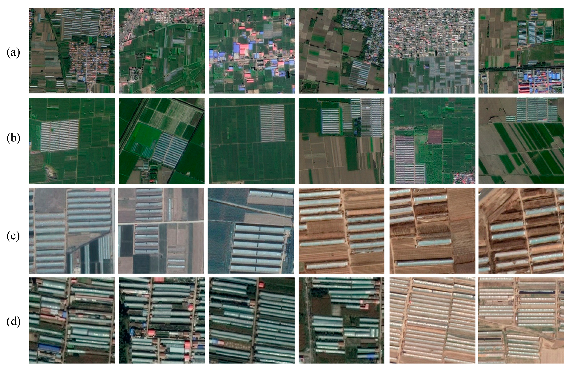
2.1. Data
2.2. Network Framework of Faster R-CNN, YOLO v3 and SSD
2.2.1. Faster R-CNN
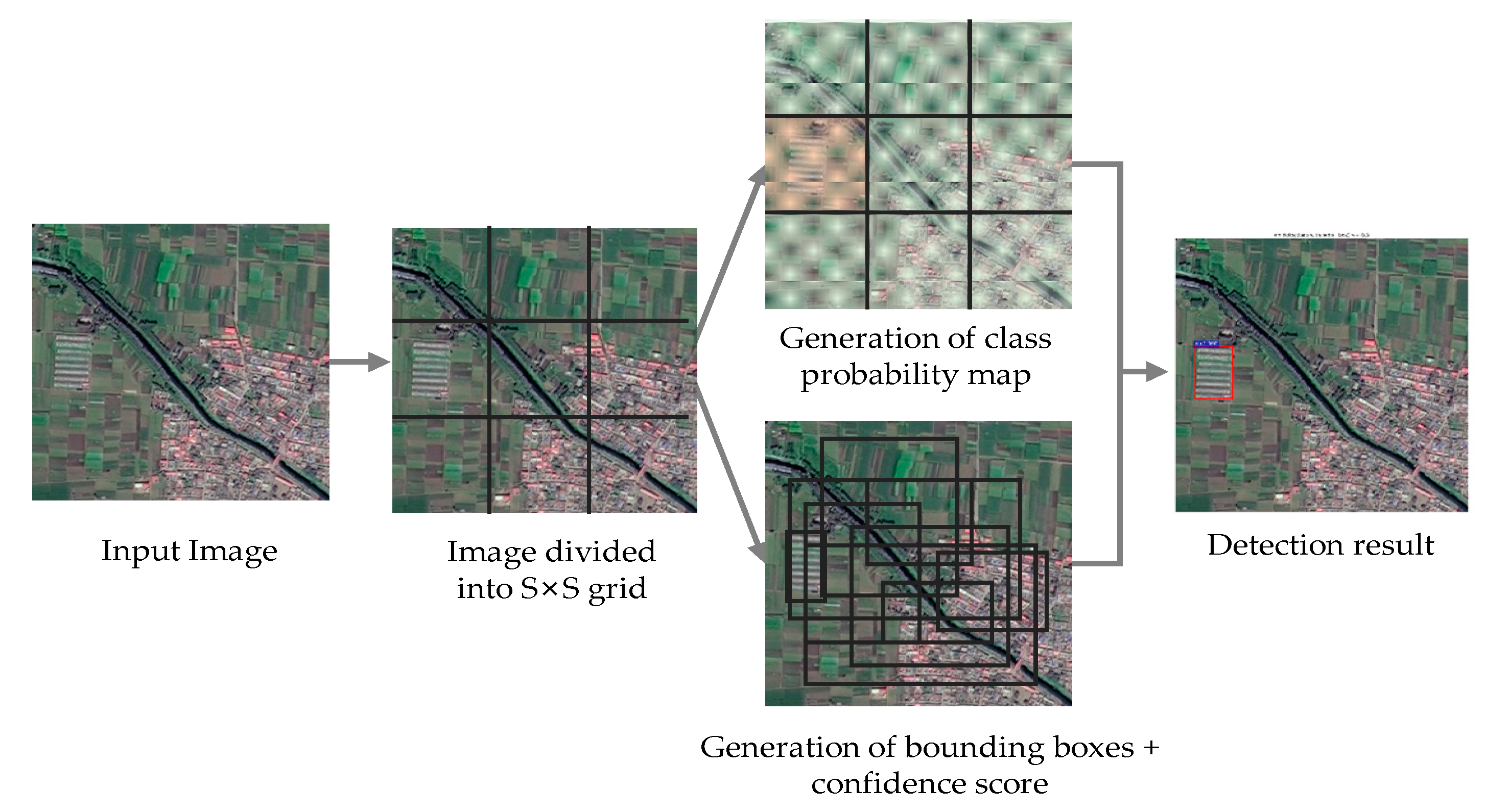
2.2.2. YOLO v3
2.2.3. SSD
2.3. Model Training
3. Results and Discussion
3.1. Evaluation Metrics
- (a)
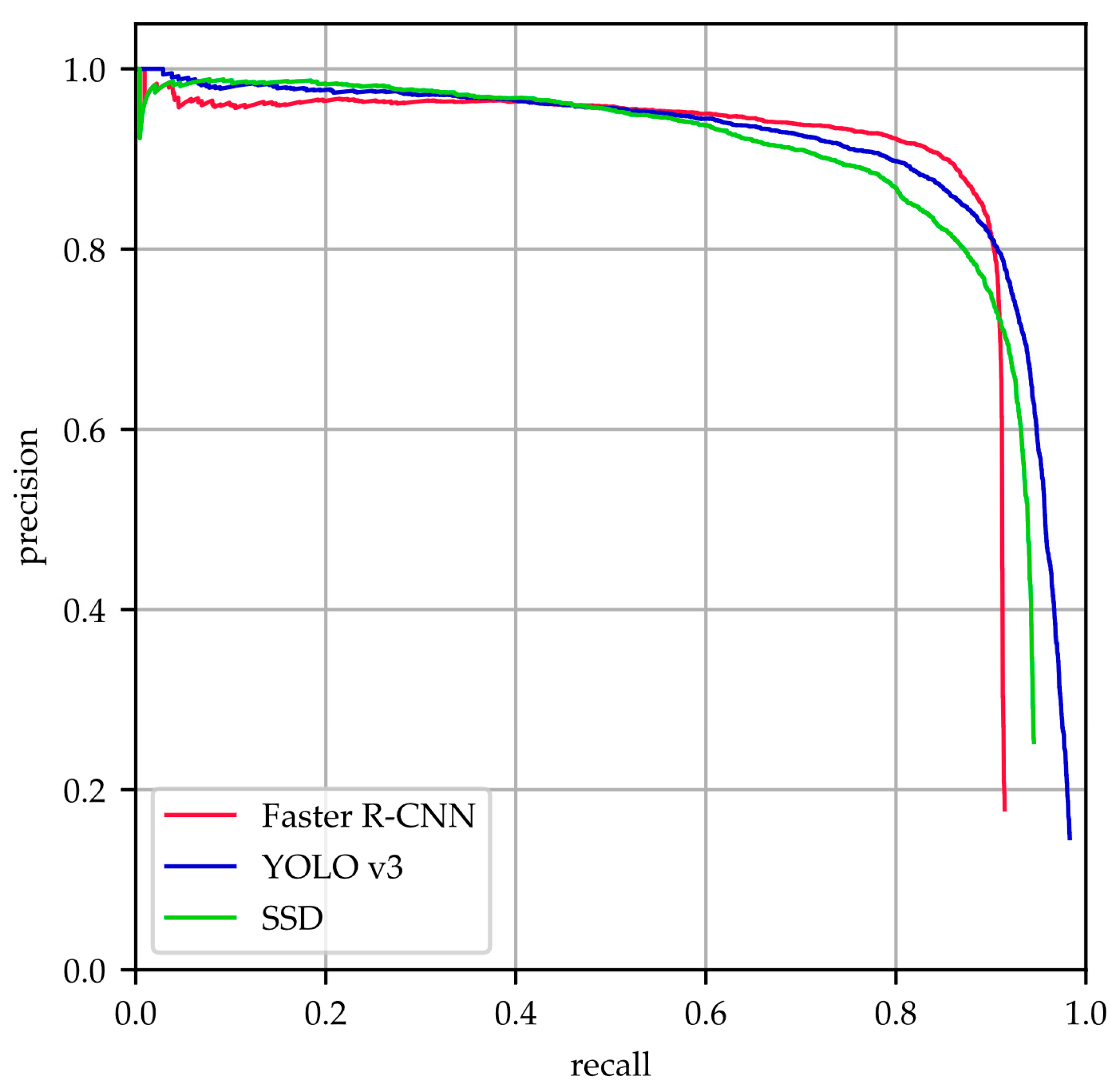
- Precision-recall curve (PRC) is composed of precision (P) and recall (R). It is a more conventional and objective judgment criterion in the field of object detection compared with individual precision or recall metric. The precision measures the fraction of correctly identified positives and detection results, while the recall measures the fraction of correctly identified positives and the total number of all ground truth samples. The precision and recall indicators are calculated as:where true positive (TP) indicates the total number of targets successfully detected by the model; false negative (FN) indicates the total number of targets that are falsely identified as other objects; false positive (FP) indicates the total number of predictions that identified other objects as targets.
- (b)
- Average precision (AP) is measured by the area under the PRC for each class. We use the mAP over all classes to evaluate the performance of the model. Since there are only two classes considered, namely AG and background, the mAP of the whole model is equal to the AP of the AG detection. Generally, the higher the mAP, the better the performance.
- (c)
- Frames per second (FPS) measures the number of images that are processed on the model per second. When running on the steady-state hardware, the larger the FPS, the faster the model detects.
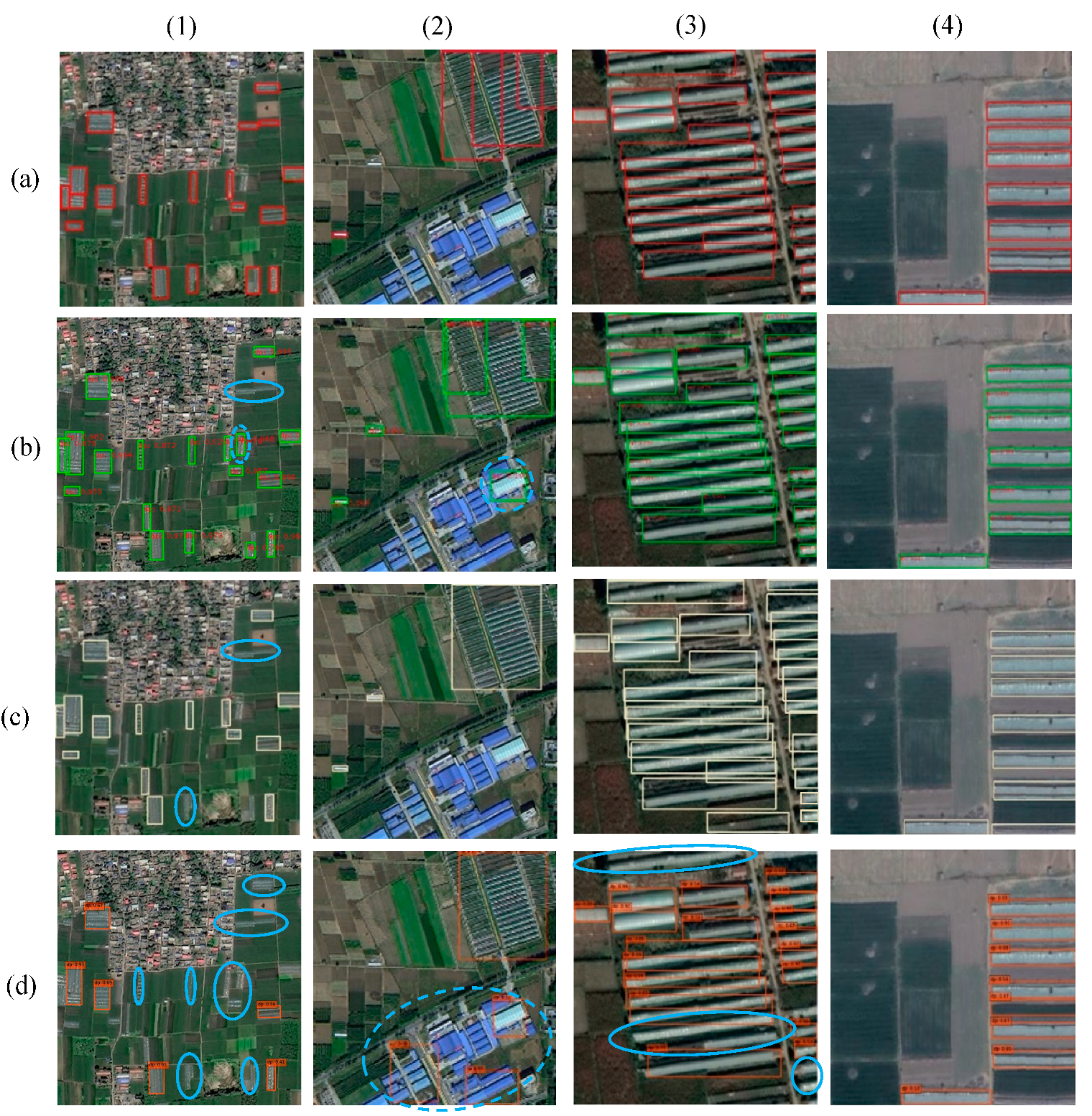
3.2. Visual Evaluation
3.3. Evaluation with Metrics
4. Conclusions
Author Contributions
Funding
Acknowledgments
Conflicts of Interest
References
- Cantliffe, D.J. Protected agriculture—A regional solution for water scarcity and production of high-value crops in the Jordan Valley. In Proceedings of the Water in the Jordan Valley: Technical Solutions and Regional Cooperation Conference, Norman, OK, USA, 13–14 November 2001; University of Oklahama: Norman, OK, USA, 2001. [Google Scholar]
- Levin, N.; Lugassi, R.; Ramon, U.; Braun, O.; Ben-Dor, E. Remote sensing as a tool for monitoring plasticulture in agricultural landscapes. Int. J. Remote Sens. 2007, 28, 183–202. [Google Scholar] [CrossRef]
- Picuno, P. Innovative material and improved technical design for a sustainable exploitation of agricultural plastic film. Polym. Plast. Technol. Eng. 2014, 53, 1000–1011. [Google Scholar] [CrossRef]
- Picuno, P.; Tortora, A.; Capobianco, R.L. Analysis of plasticulture landscapes in Southern Italy through remote sensing and solid modelling techniques. Landsc. Urban Plan. 2011, 100, 45–56. [Google Scholar] [CrossRef]
- Chaofan, W.; Jinsong, D.; Ke, W.; Ligang, M.; Tahmassebi, A.R.S. Object-based classification approach for greenhouse mapping using Landsat-8 imagery. Int. J. Agric. Biol. Eng. 2016, 9, 79–88. [Google Scholar]
- Knickel, K. Changes in Farming Systems, Landscape, and Nature: Key Success Factors of Agri-Environmental Schemes (AES). In Proceedings of the EUROMAB Symposium, Vienna, Austria, 15–16 September 1999. [Google Scholar]
- Du, X.M.; Wu, Z.H.; Zhang, Y.Q.; PEI, X.X. Study on changes of soil salt and nutrient in greenhouse of different planting years. J. Soil Water Conserv. 2007, 2, 78–80. [Google Scholar]
- Hanan, J.J.; Holley, W.D.; Goldsberry, K.L. Greenhouse Management; Springer Science & Business Media: New York, NY, USA, 2012. [Google Scholar]
- Arel, I.; Rose, D.C.; Karnowski, T.P. Deep machine learning-a new frontier in artificial intelligence research [research frontier]. IEEE Comput. Intell. Mag. 2010, 5, 13–18. [Google Scholar] [CrossRef]
- Bishop, C.M. Pattern Recognition and Machine Learning; Jordan, M., Kleinberg, J., Schölkopf, B., Eds.; Inf. Sci. Stat.: Cambridge, UK, 2007. [Google Scholar]
- Ma, Y.; Wu, H.; Wang, L.; Huang, B.; Ranjan, R.; Zomaya, A.; Jie, W. Remote sensing big data computing: Challenges and opportunities. Future Gener. Comput. Syst. 2015, 51, 47–60. [Google Scholar] [CrossRef]
- Benediktsson, J.A.; Chanussot, J.; Moon, W.M. Very High-Resolution Remote Sensing: Challenges and Opportunities. Proc. IEEE 2012, 100, 1907–1910. [Google Scholar] [CrossRef]
- LeCun, Y.; Bengio, Y.; Hinton, G. Deep Learning. Nature 2015, 521, 436–444. [Google Scholar] [CrossRef]
- Li, H. Deep learning for natural language processing: Advantages and challenges. Natl. Sci. Rev. 2017, 5, 24–26. [Google Scholar] [CrossRef]
- Otter, D.W.; Medina, J.R.; Kalita, J.K. A survey of the usages of deep learning for natural language processing. IEEE Trans. Neural Netw. Learn. Syst. 2020, 1–21. [Google Scholar] [CrossRef] [PubMed]
- Brunetti, A.; Buongiorno, D.; Trotta, G.F.; Bevilacqua, V. Computer vision and deep learning techniques for pedestrian detection and tracking: A survey. Neurocomputing 2018, 300, 17–33. [Google Scholar] [CrossRef]
- Silver, D.; Huang, A.; Maddison, C.J.; Guez, A.; Sifre, L.; Van Den Driessche, G.; Dieleman, S. Mastering the game of Go with deep neural networks and tree search. Nature 2016, 529, 484–489. [Google Scholar] [CrossRef] [PubMed]
- Chen, Y.; Fan, R.; Yang, X.; Wang, J.; Latif, A. Extraction of urban water bodies from high-resolution remote-sensing imagery using deep learning. Water 2018, 10, 585. [Google Scholar] [CrossRef]
- Gao, L.; Song, W.; Dai, J.; Chen, Y. Road extraction from high-resolution remote sensing imagery using refined deep residual convolutional neural network. Remote Sens. 2019, 11, 552. [Google Scholar] [CrossRef]
- Alshehhi, R.; Marpu, P.R.; Woon, W.L.; Dalla Mura, M. Simultaneous extraction of roads and buildings in remote sensing imagery with convolutional neural networks. ISPRS J. Photogramm. Remote Sens. 2017, 130, 139–149. [Google Scholar] [CrossRef]
- Kamel, A.; Sheng, B.; Yang, P.; Li, P.; Shen, R.; Feng, D.D. Deep convolutional neural networks for human action recognition using depth maps and postures. IEEE Trans. Syst. Man Cybern. Syst. 2018, 49, 1806–1819. [Google Scholar] [CrossRef]
- Xu, Y.; Xie, Z.; Feng, Y.; Chen, Z. Road extraction from high-resolution remote sensing imagery using deep learning. Remote Sens. 2018, 10, 1461. [Google Scholar] [CrossRef]
- Maggiori, E.; Tarabalka, Y.; Charpiat, G.; Alliez, P. Convolutional neural networks for large-scale remote-sensing image classification. IEEE Trans. Geosci. Remote Sens. 2016, 55, 645–657. [Google Scholar] [CrossRef]
- Pan, X.; Zhao, J. High-resolution remote sensing image classification method based on convolutional neural network and restricted conditional random field. Remote Sens. 2018, 10, 920. [Google Scholar] [CrossRef]
- Wang, Y.; Wang, C.; Zhang, H.; Dong, Y.; Wei, S. Automatic Ship Detection Based on RetinaNet Using Multi-Resolution Gaofen-3 Imagery. Remote Sens. 2019, 11, 531. [Google Scholar] [CrossRef]
- Chen, C.; Gong, W.; Chen, Y.; Li, W. Learning a two-stage CNN model for multi-sized building detection in remote sensing images. Remote Sens. Lett. 2019, 10, 103–110. [Google Scholar] [CrossRef]
- Koga, Y.; Miyazaki, H.; Shibasaki, R. A Method for Vehicle Detection in High-Resolution Satellite Images that Uses a Region-Based Object Detector and Unsupervised Domain Adaptation. Remote Sens. 2020, 12, 575. [Google Scholar] [CrossRef]
- Girshick, R.; Donahue, J.; Darrell, T.; Malik, J. Rich feature hierarchies for accurate object detection and semantic segmentation. In Proceedings of the IEEE Conference on Computer Vision and Pattern Recognition, Columbus, OH, USA, 20–23 June 2014. [Google Scholar]
- Girshick, R. Fast r-cnn. In Proceedings of the IEEE International Conference on Computer Vision, Santiago, Chile, 11–18 December 2015. [Google Scholar]
- Ren, S.; He, K.; Girshick, R.; Sun, J. Faster r-cnn: Towards real-time object detection with region proposal networks. IEEE Trans. Pattern Anal. Mach. Intell. 2017, 39, 1137–1149. [Google Scholar] [CrossRef] [PubMed]
- Liu, W.; Anguelov, D.; Erhan, D.; Szegedy, C.; Reed, S.; Fu, C.Y.; Berg, A.C. Ssd: Single shot multibox detector. In Proceedings of the European Conference on Computer Vision—ECCV2016, Amsterdam, The Netherlands, 8–16 October 2016. [Google Scholar]
- Redmon, J.; Divvala, S.; Girshick, R.; Farhadi, A. You only look once: Unified, real-time object detection. In Proceedings of the IEEE Conference on Computer Vision and Pattern Recognition, Las Vegas, NV, USA, 27–30 June 2016. [Google Scholar]
- Redmon, J.; Farhadi, A. YOLO9000: Better, faster, stronger. In Proceedings of the IEEE Conference on Computer Vision and Pattern Recognition, Honolulu, HI, USA, 21–26 July 2017. [Google Scholar]
- Redmon, J.; Farhadi, A. YOLOv3: An Incremental Improvement. Available online: https://arxiv.org/abs/1804.02767 (accessed on 31 August 2020).
- Everingham, M.; Van Gool, L.; Williams, C.K.; Winn, J.; Zisserman, A. The Pascal Visual Object Classes (VOC) Challenge. Int. J. Comput. Vis. 2010, 88, 303–338. [Google Scholar] [CrossRef]
- Deng, J.; Dong, W.; Socher, R.; Li, L.J.; Li, K.; Fei-Fei, L. ImageNet: A large-scale hierarchical image database. In Proceedings of the IEEE Conference on Computer Vision and Pattern Recognition, Miami, FL, USA, 20–25 June 2009; pp. 248–255. [Google Scholar]
- Lin, T.Y.; Maire, M.; Belongie, S.; Hays, J.; Perona, P.; Ramanan, D.; Zitnick, C.L. Microsoft COCO: Common Objects in Context. In Lecture Notes in Computer Science, Proceedings of the European Conference on Computer Vision—ECCV2014, Zurich, Switzerland, 6–12 September 2014; Springer: Cham, Switzerland, 2014; Volume 8693, pp. 740–755. [Google Scholar]
- Cheng, G.; Zhou, P.; Han, J. Learning rotation-invariant convolutional neural networks for object detection in VHR optical remote sensing images. IEEE Trans. Geosci. Remote Sens. 2016, 54, 7405–7415. [Google Scholar] [CrossRef]
- Guo, W.; Yang, W.; Zhang, H.; Hua, G. Geospatial object detection in high resolution satellite images based on multi-scale convolutional neural network. Remote Sens. 2018, 10, 131. [Google Scholar] [CrossRef]
- Zhang, S.; Wu, R.; Xu, K.; Wang, J.; Sun, W. R-CNN-Based Ship Detection from High Resolution Remote Sensing Imagery. Remote Sens. 2019, 11, 631. [Google Scholar] [CrossRef]
- Chen, Z.; Zhang, T.; Ouyang, C. End-to-end airplane detection using transfer learning in remote sensing images. Remote Sens. 2018, 10, 139. [Google Scholar] [CrossRef]
- Ma, H.; Liu, Y.; Ren, Y.; Yu, J. Detection of Collapsed Buildings in Post-Earthquake Remote Sensing Images Based on the Improved YOLOv3. Remote Sens. 2019, 12, 44. [Google Scholar] [CrossRef]
- Paisitkriangkrai, S.; Sherrah, J.; Janney, P.; Hengel, V.D. Effective semantic pixel labelling with convolutional networks and Conditional Random Fields. In Proceedings of the IEEE Conference on Computer Vision and Pattern Recognition Workshops, Boston, MA, USA, 7–12 June 2015; pp. 36–43. [Google Scholar]
- Simonyan, K.; Zisserman, A. Very Deep Convolutional Networks for Large-Scale Image Recognition. arXiv 2014, arXiv:1409.1556. [Google Scholar]
- West, J.; Ventura, D.; Warnick, S. Spring Research Presentation: A Theoretical Foundation for Inductive Transfer; Brigham Young University, College of Physical and Mathematical Sciences: Provo, UT, USA, 2007; Volume 1. [Google Scholar]
- Bochkovskiy, A.; Wang, C.Y.; Liao, H.Y.M. YOLOv4: Optimal Speed and Accuracy of Object Detection. arXiv 2020, arXiv:2004.10934. [Google Scholar]


| Data Source | Spatial Resolution | Number of Total Samples | Number of Target AGs | Number of Training Samples | Number of Validation Samples | Number of Test Samples |
|---|---|---|---|---|---|---|
| GF-1 | 2 m | 413 | 14,920 | 247 | 83 | 83 |
| GF-2 | 1 m | 964 | 3465 | 578 | 193 | 193 |
| Total | 1377 | 18,385 | 825 | 276 | 276 |
| Faster R-CNN | YOLO v3 | SSD | |
|---|---|---|---|
| Phases | RPN + Fast R-CNN detector | Concurrent bounding-box regression and classification | Concurrent bounding-box regression and classification |
| Neural Network Type | Fully convolutional | Fully convolutional | Fully convolutional |
| Backbone Feature Extractor | VGG-16 or other feature extractors | Darknet-53 (53 convolutional layers) | VGG-16 or other feature extractors |
| Location Detection | Anchor-based | Anchor-Based | Prior boxes/Default boxes |
| Anchor Box | 9 default boxes with different scales and aspect ratios | K-means from coco and VOC, 9 anchors boxes with different size | A fixed number of bounding boxes with different scales and aspect ratios in each feature map |
| IoU Thresholds | Two (at 0.3 and 0.7) | One (at 0.5) | One (at 0.5) |
| Loss Function | Softmax loss for classification; Smooth L1 for regression | Binary cross-entropy loss | Softmax loss for confidence; Smooth L1 Loss for localization |
| Input Size | Conserve the aspect ratio of the original image, and resized dimension ranges from smallest 500 to largest 1000 | Random multi-scale input | Resize original images to a fixed size (300 × 300 or 512 × 512) |
| Faster R-CNN | YOLO v3 | SSD | |
|---|---|---|---|
| mAP (GF-1& GF-2) | 86.0% | 90.4% | 84.9% |
| mAP (GF-1) | 64.0% | 73.0% | 60.9% |
| mAP (GF-2) | 88.3% | 93.2% | 87.9% |
| FPS | 12 | 73 | 35 |
© 2020 by the authors. Licensee MDPI, Basel, Switzerland. This article is an open access article distributed under the terms and conditions of the Creative Commons Attribution (CC BY) license (http://creativecommons.org/licenses/by/4.0/).
Share and Cite
Li, M.; Zhang, Z.; Lei, L.; Wang, X.; Guo, X. Agricultural Greenhouses Detection in High-Resolution Satellite Images Based on Convolutional Neural Networks: Comparison of Faster R-CNN, YOLO v3 and SSD. Sensors 2020, 20, 4938. https://doi.org/10.3390/s20174938
Li M, Zhang Z, Lei L, Wang X, Guo X. Agricultural Greenhouses Detection in High-Resolution Satellite Images Based on Convolutional Neural Networks: Comparison of Faster R-CNN, YOLO v3 and SSD. Sensors. 2020; 20(17):4938. https://doi.org/10.3390/s20174938
Chicago/Turabian StyleLi, Min, Zhijie Zhang, Liping Lei, Xiaofan Wang, and Xudong Guo. 2020. "Agricultural Greenhouses Detection in High-Resolution Satellite Images Based on Convolutional Neural Networks: Comparison of Faster R-CNN, YOLO v3 and SSD" Sensors 20, no. 17: 4938. https://doi.org/10.3390/s20174938
APA StyleLi, M., Zhang, Z., Lei, L., Wang, X., & Guo, X. (2020). Agricultural Greenhouses Detection in High-Resolution Satellite Images Based on Convolutional Neural Networks: Comparison of Faster R-CNN, YOLO v3 and SSD. Sensors, 20(17), 4938. https://doi.org/10.3390/s20174938