Blind First-Order Perspective Distortion Correction Using Parallel Convolutional Neural Networks


Abstract
:1. Introduction
- Our network architecture corrects perspective distortion and produces visually better images than other state-of-the-art methods. In terms of pixel-wise reconstruction error, our method outperforms other works.
- Our method, to the best of our knowledge, is the first attempt to estimate the transformation matrix for correcting an image rather than using a reconstruction-based approach. Our method is straightforward and the network design is simpler compared to other works that mainly rely on deep generative models such as GANs or encoder-decoder networks, which are notoriously difficult to train and prone to instability.
- Our method also recovers the original scale and proportion of the image. This is not observed in other works. Recovering the scale and proportion is beneficial for applications that perform distance measurements.
2. Related Work
2.1. Model-Based Techniques
2.2. Methods Using Low-Level Features
2.3. Learning-Based Methods
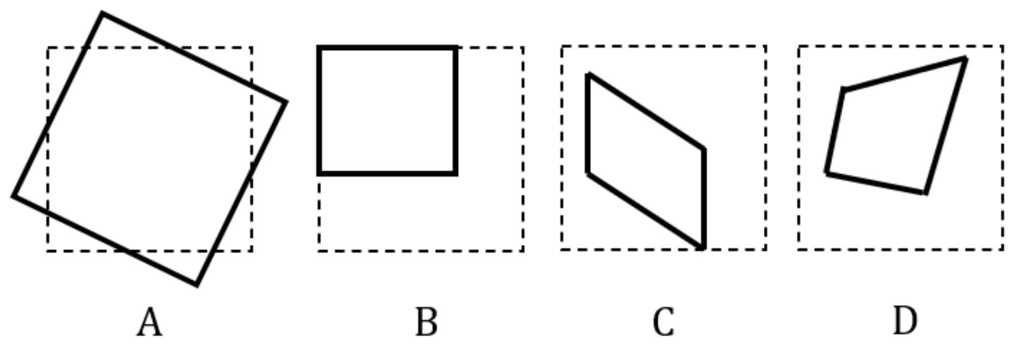
3. Empirical Analysis on the Transformation Matrix
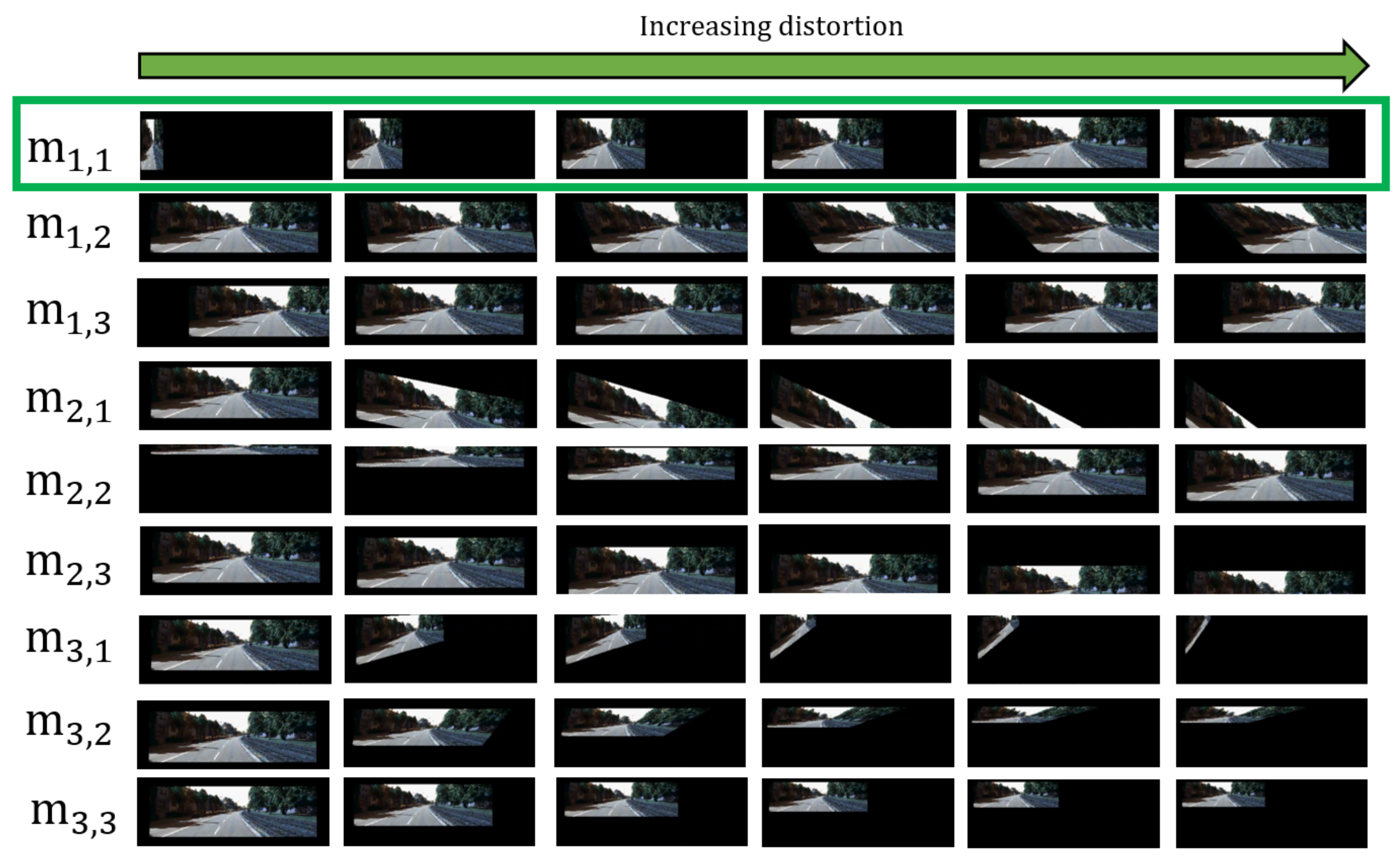
- Small changes in result in a sideways rotation along the Y axis. Small changes in result in a shearing operation, where the image’s bottom left and bottom right anchor points move sideways and upwards. Equation (3) shows that increasing and causes the and to shrink. This is represented as an element pair, .
- Based in Equation (3), , , deal with the scale of the image. The matrix entries, and , deal with the width and height of the image respectively. Since is part of the denominator, it changes both the width and height of the image. We do not need to use as input when training our network because and can be inferred instead. This is represented as an element pair, .
- Since is multiplied by y and is multiplied by x in Equation (3), this creates a shearing effect along and respectively. This is represented as an element pair, .
- Since no other term is multiplied with and in Equation (3), increasing these entries results in pixel-wise displacements along x and y respectively. These are not considered as input for the network as they are typically not observed in distorted images.
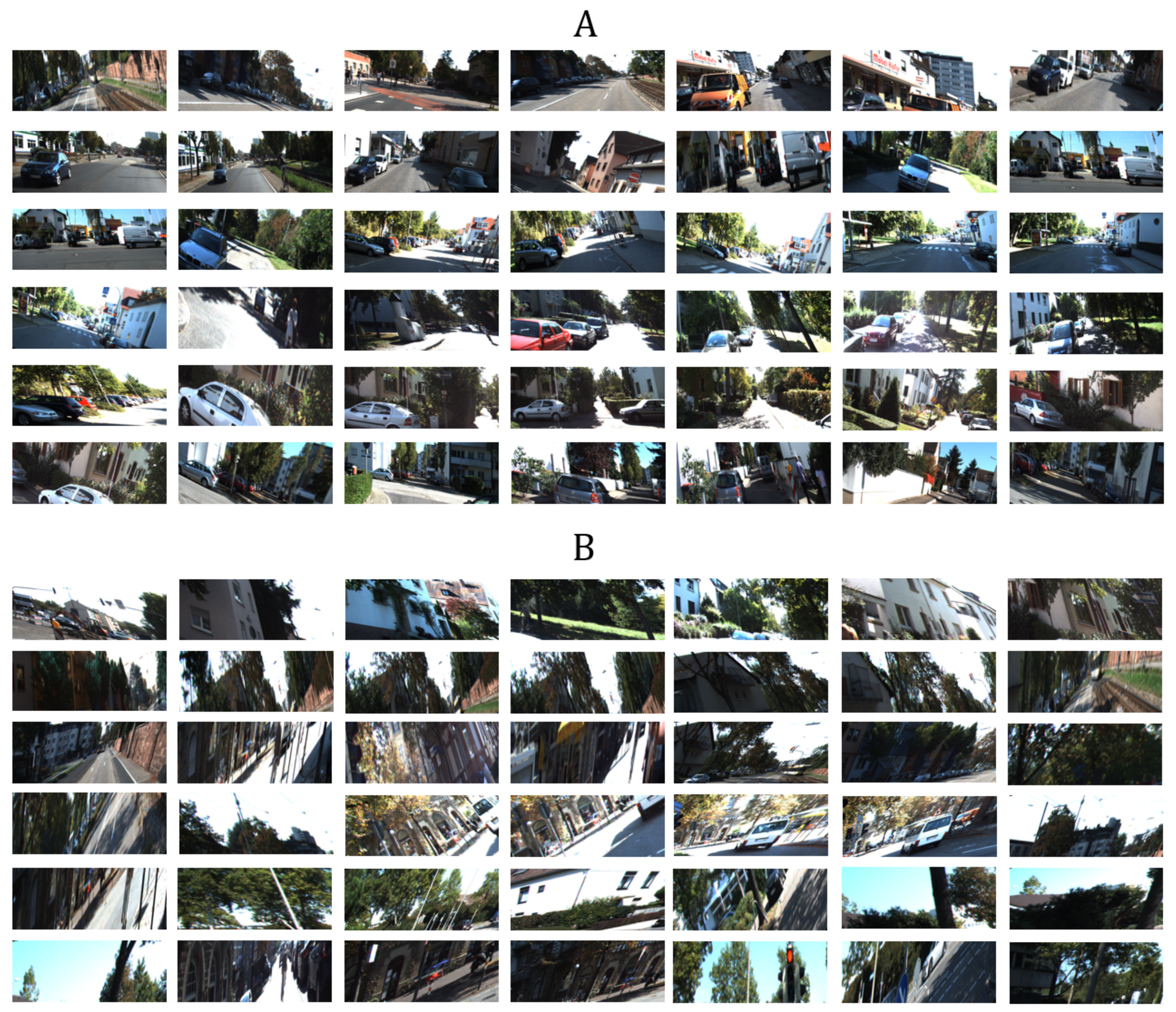
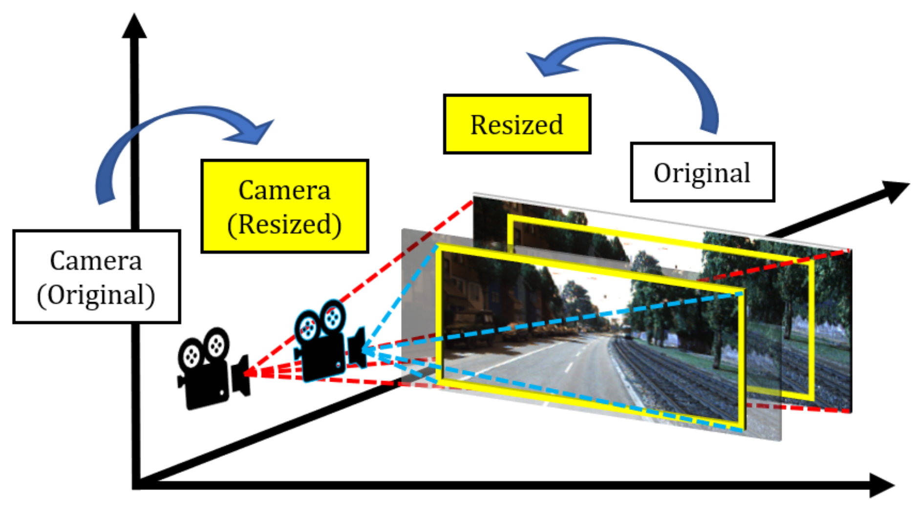
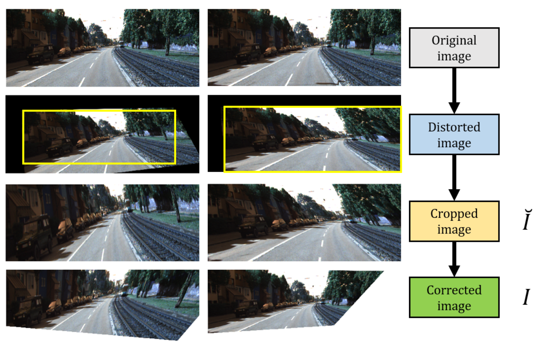
4. Synthetic Distortion Dataset: dKITTI
- Declare a bounding box B with a size of in terms of width and height. where W refers to the distorted image generated.
- Iteratively decrease until the number of zero pixels, P, becomes 0. B becomes the selected cropped image .
- Resize by bilinear interpolation such that where O is the original image.
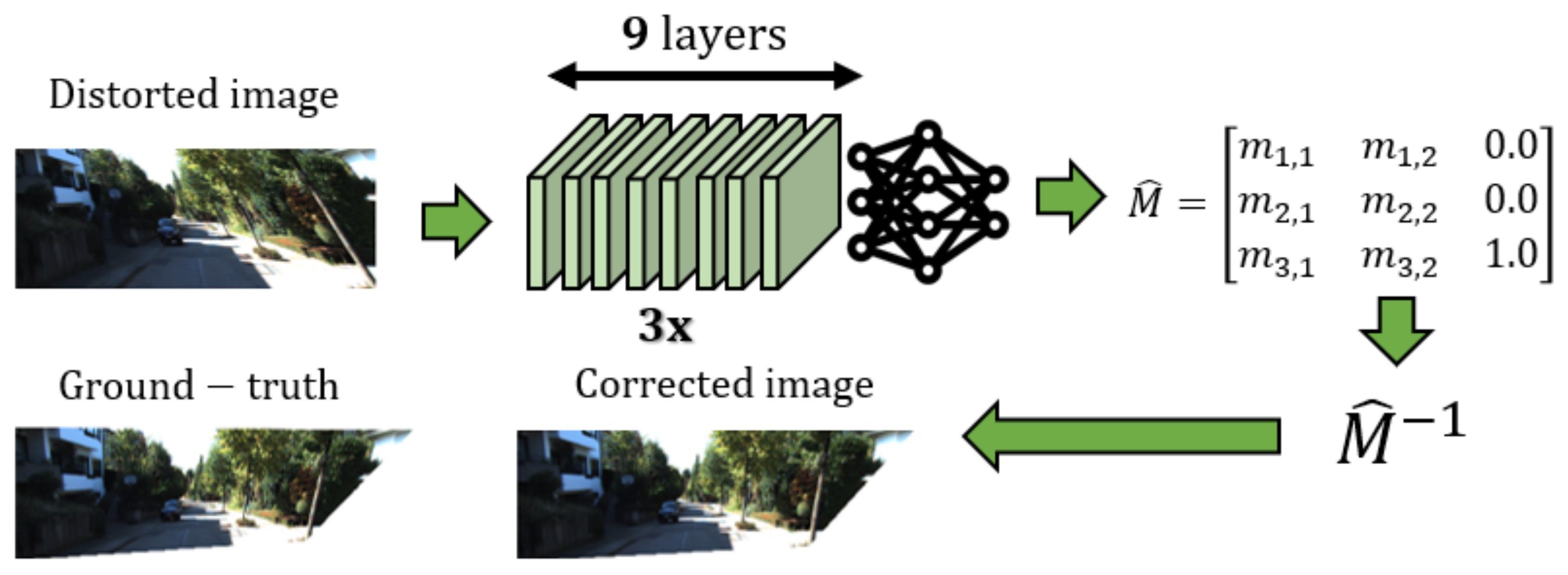
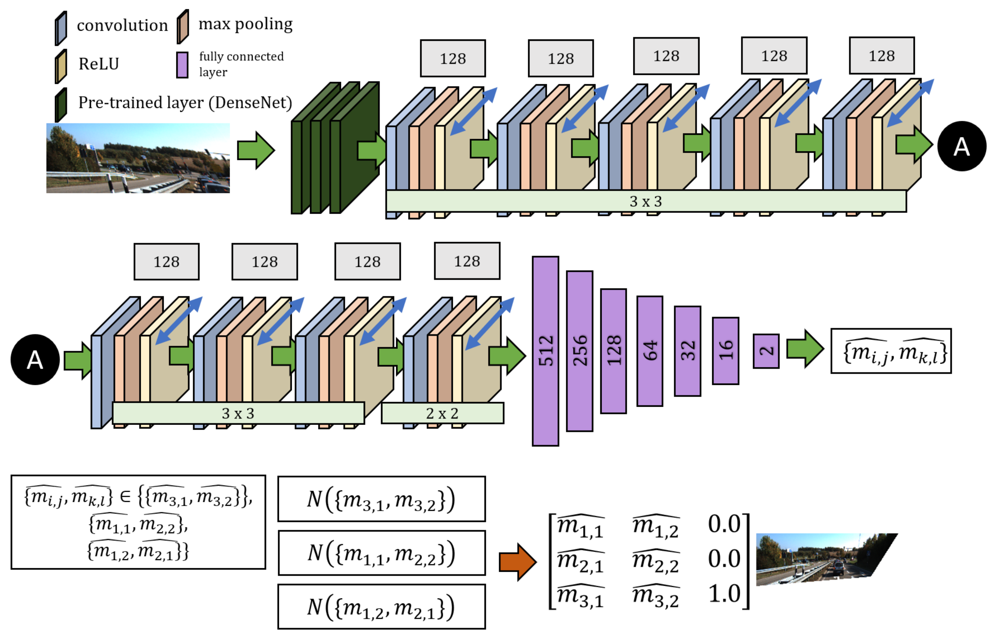
5. Proposed Network
5.1. Parallel CNN Model
5.2. Training Details
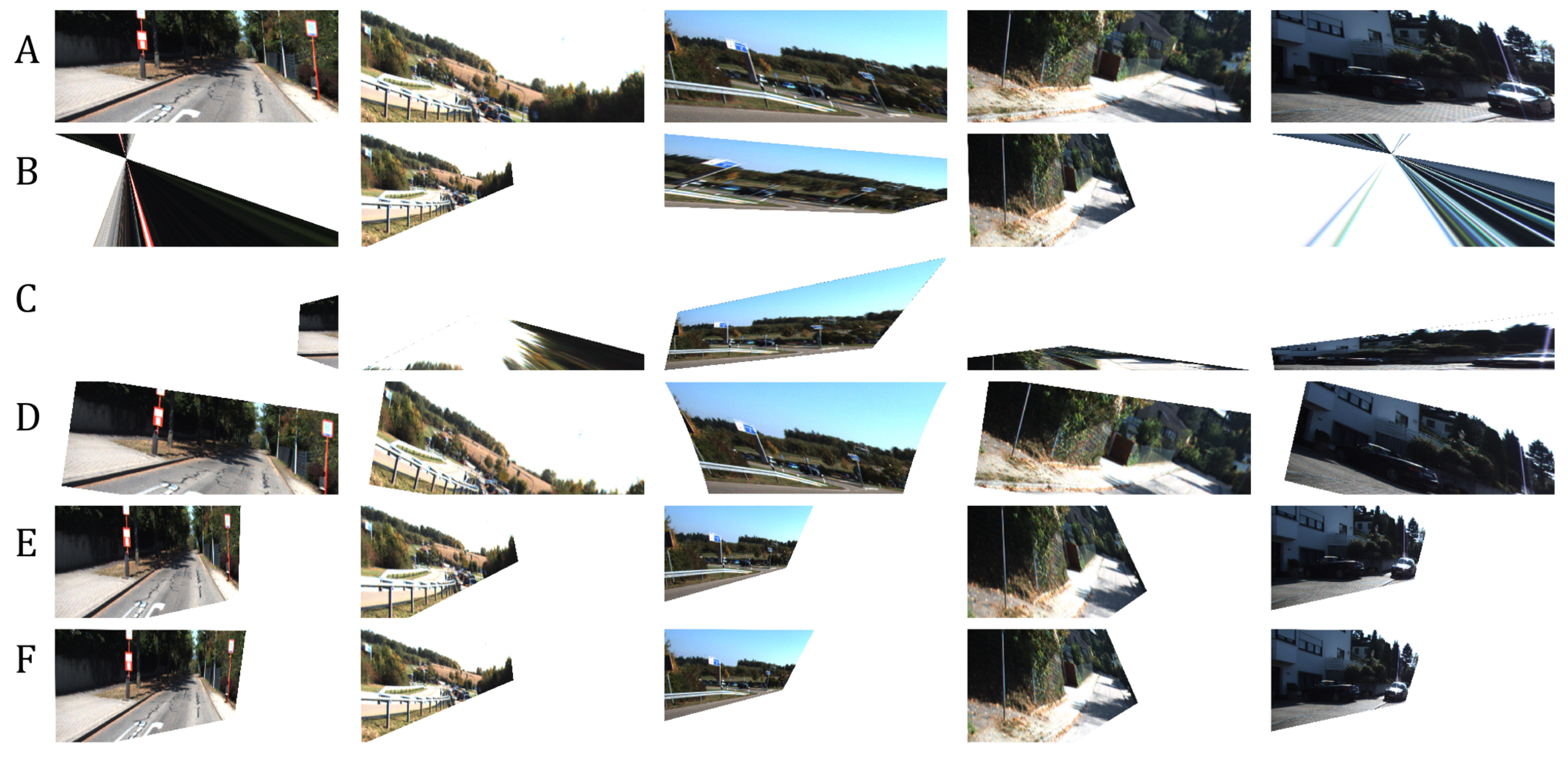
6. Evaluation
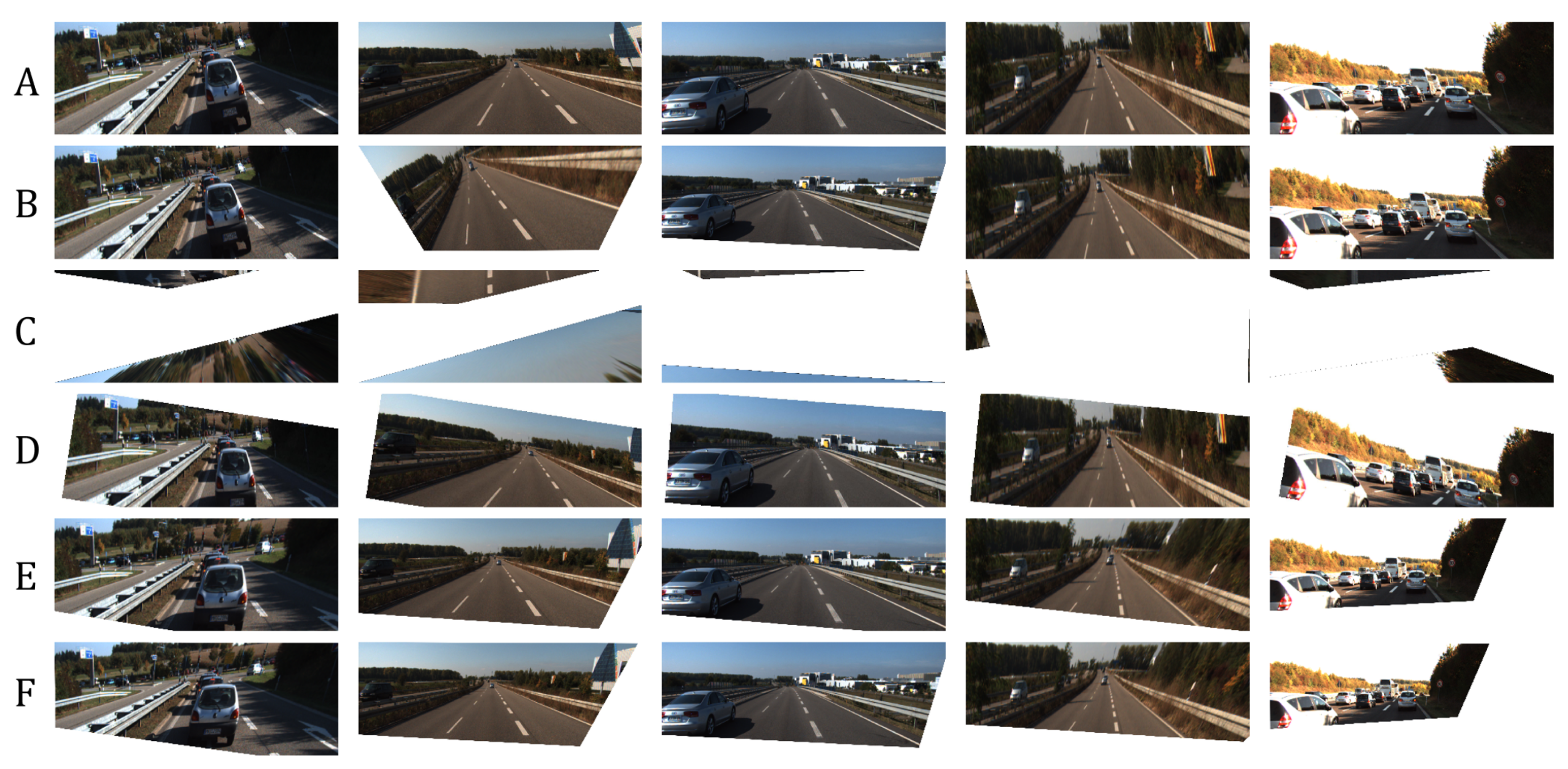
- Both methods do not consider the scaling of images as a possible factor in perspective distortion, unlike our method, as discussed in Section 3.
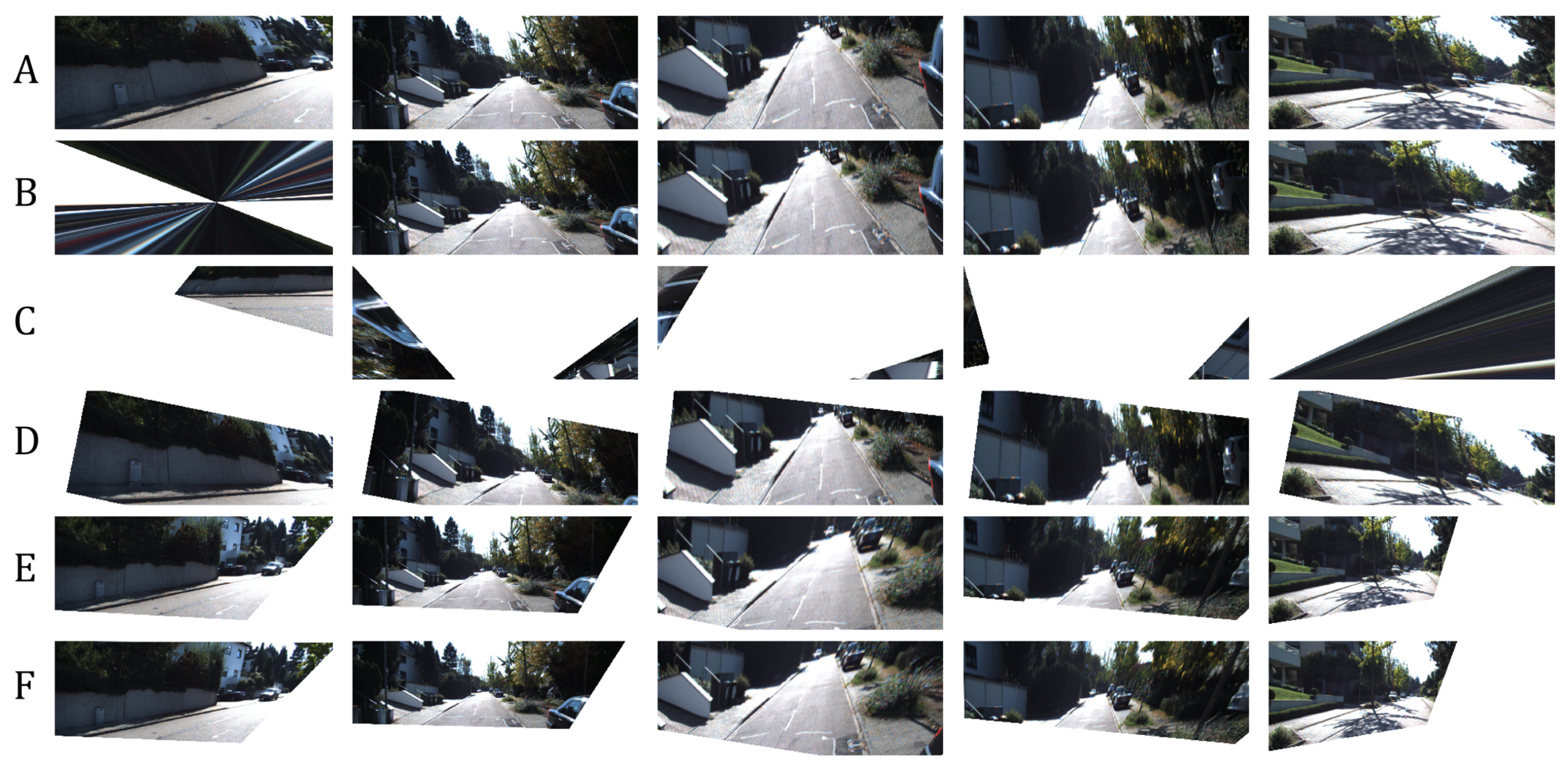
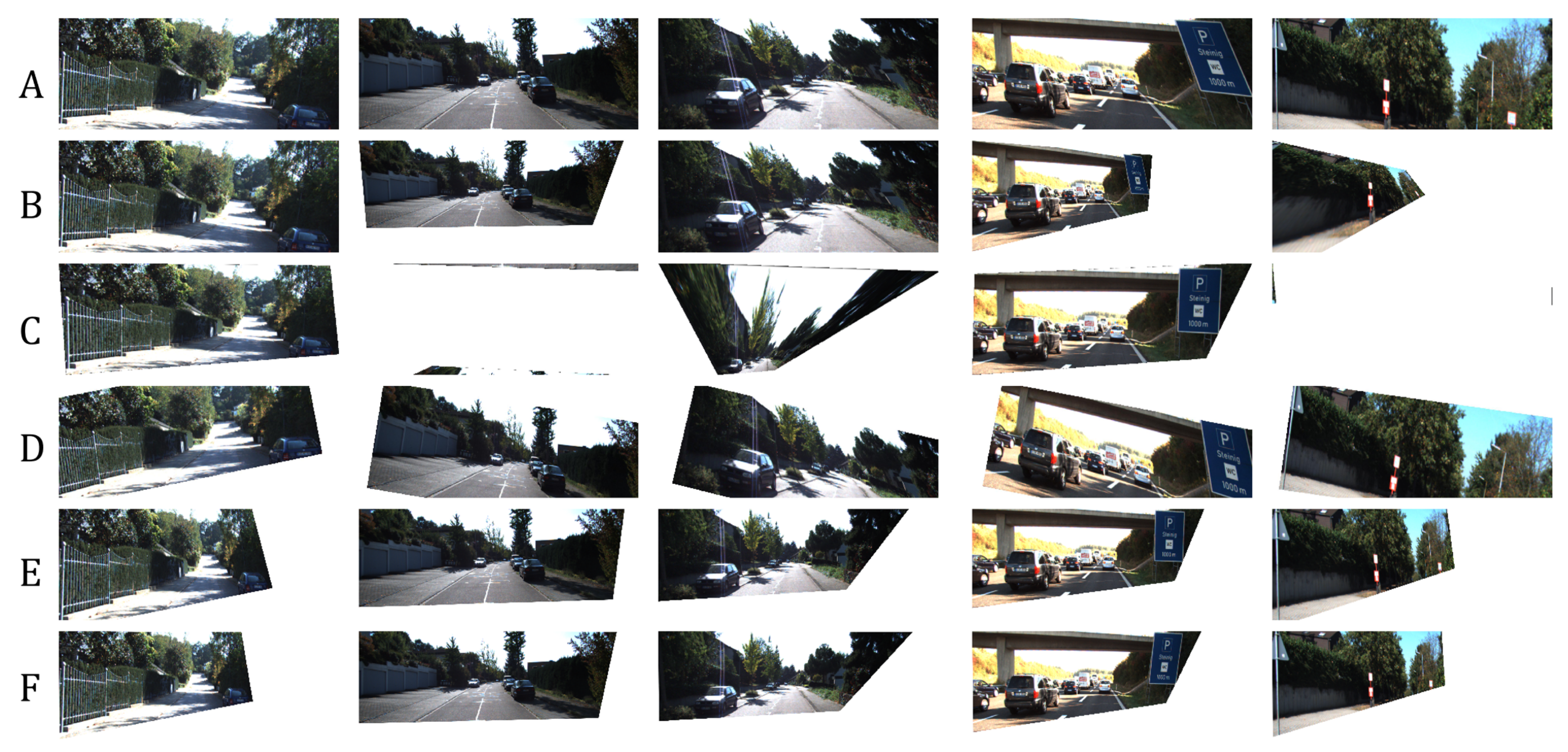
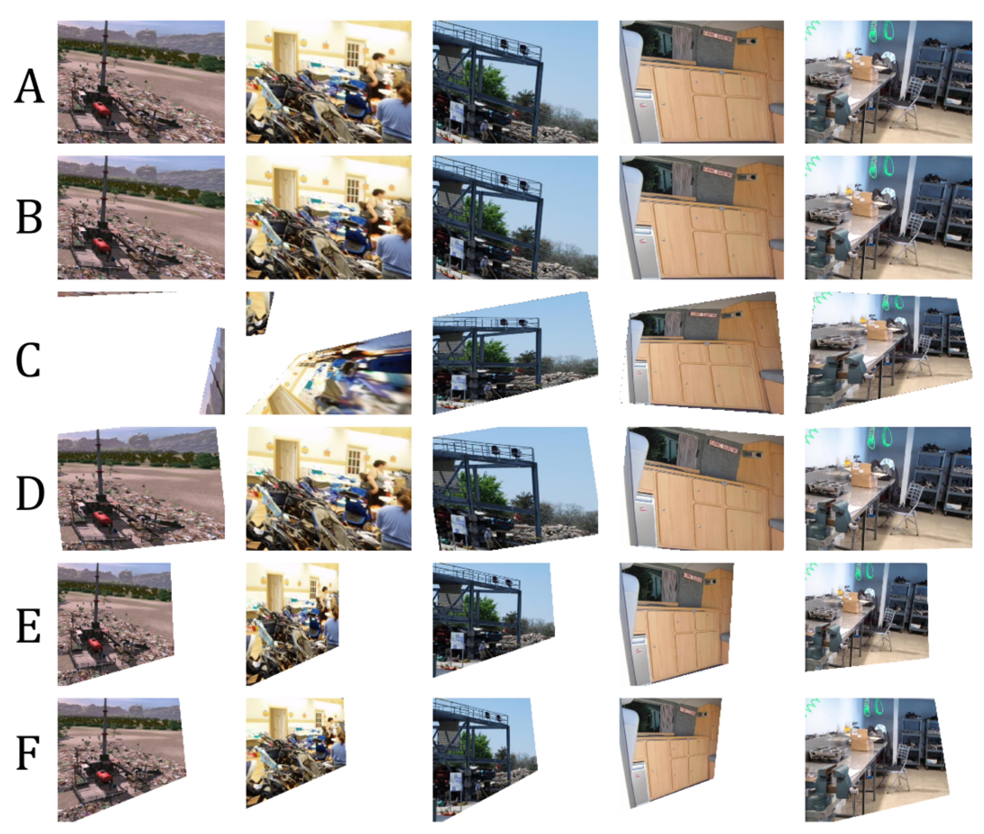
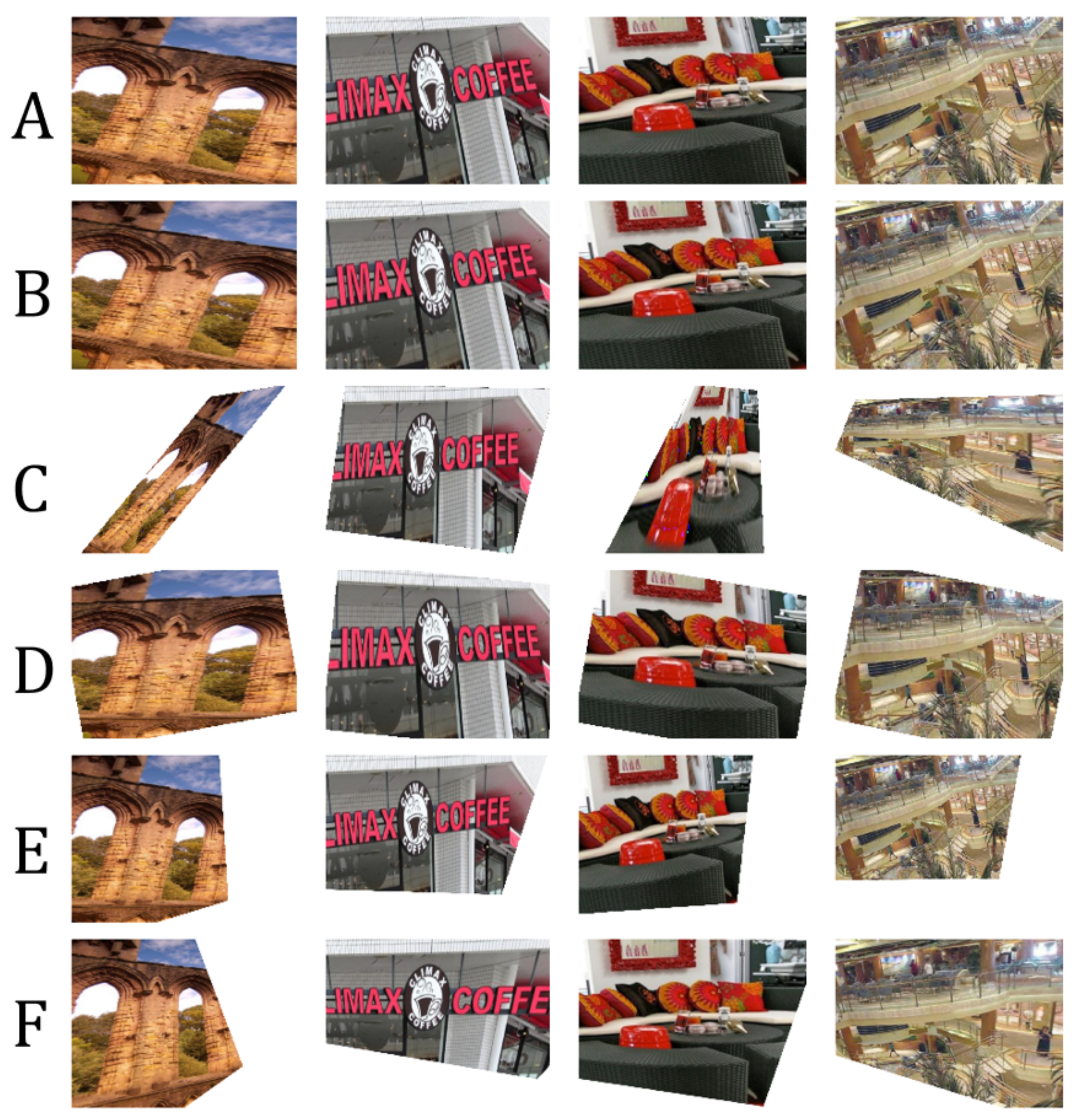
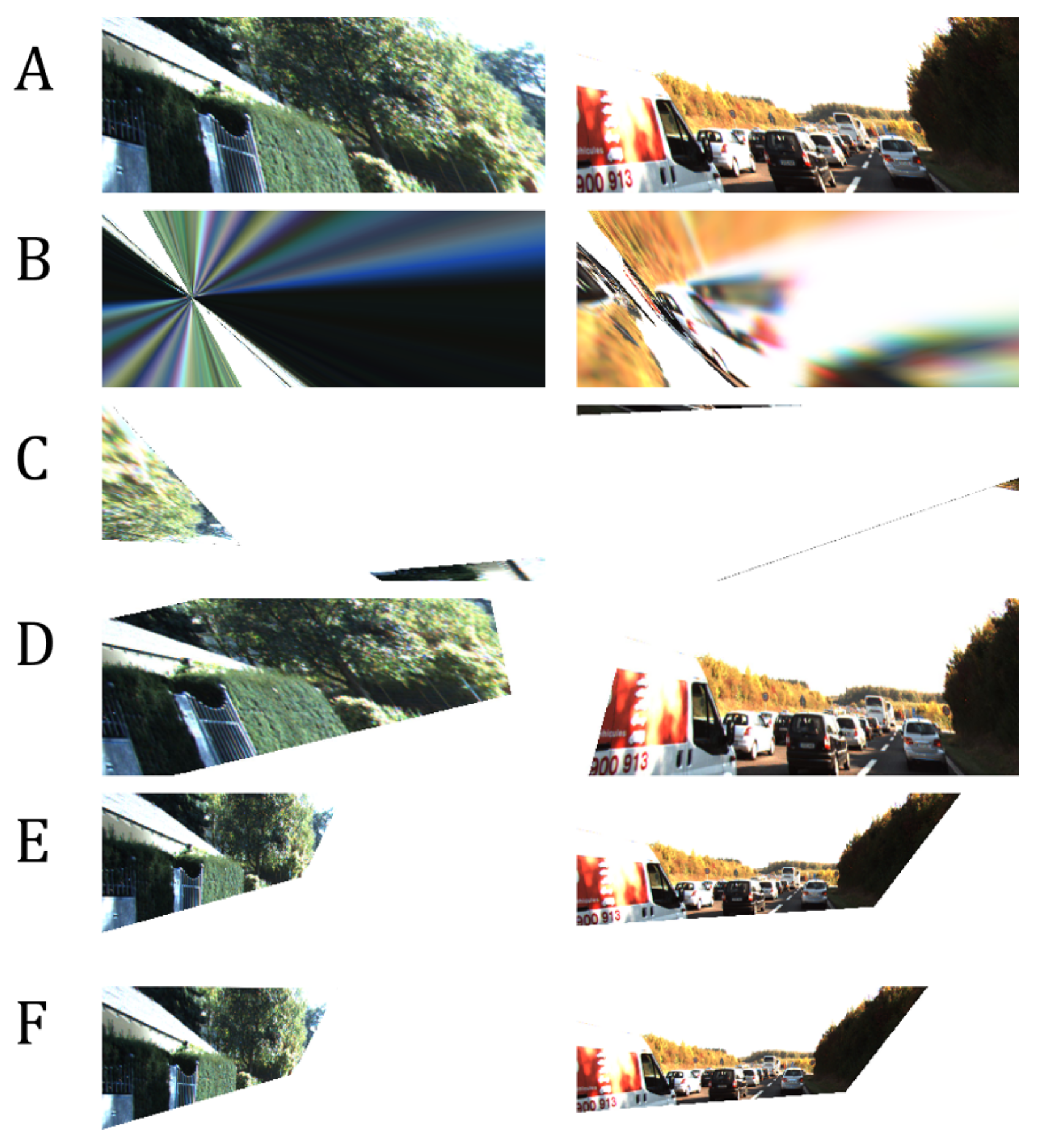
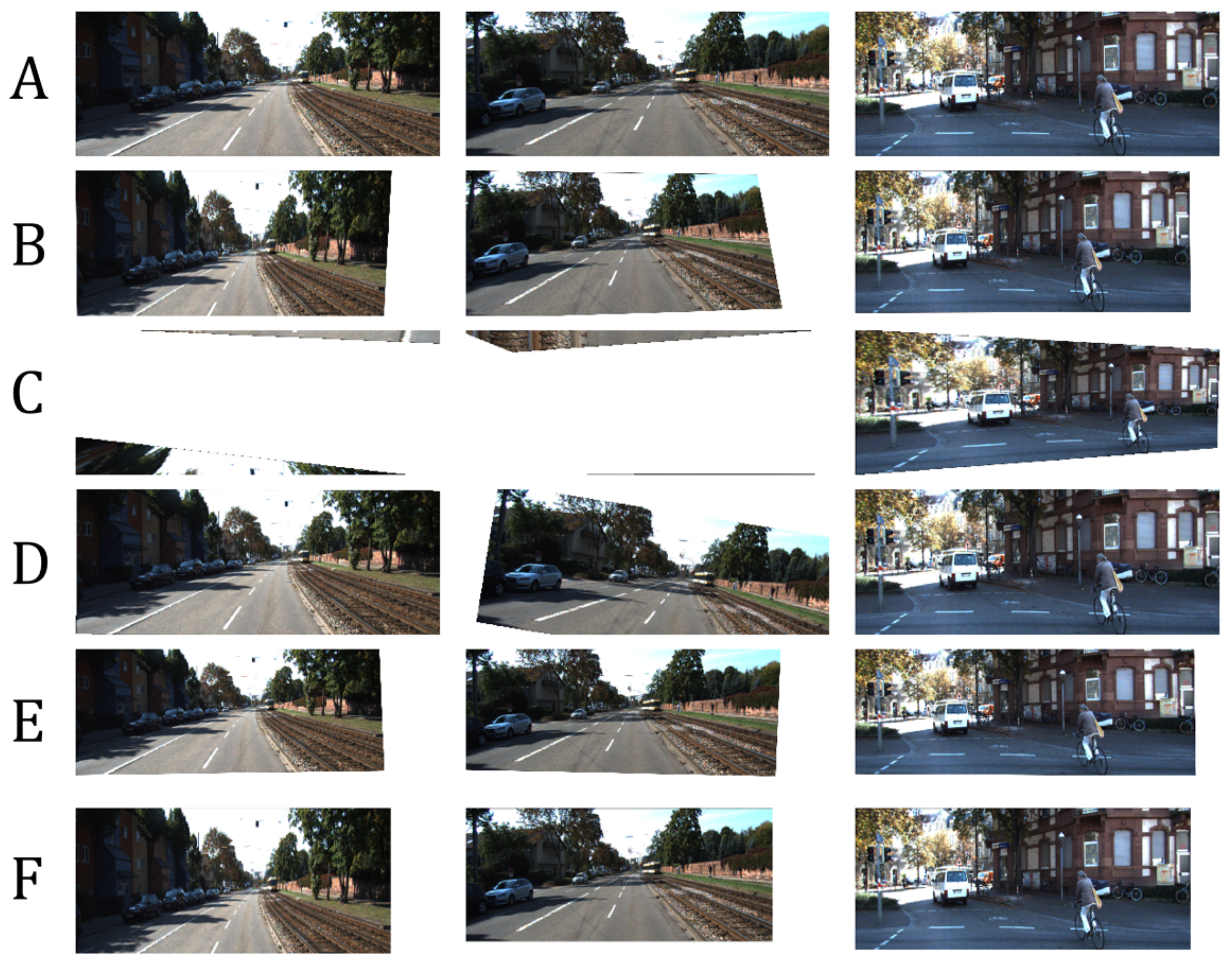
- Some images are misclassified as a different distortion type using the method of Li et al. [11]. For example in Figure 8, the third image of row A is misclassified as a barrel or pincushion distortion which resulted in a different corrected image. Our method covers more cases of perspective distortions. As seen in our results, our method consistently produces corrected images.
6.1. Experiment on Network Variants
6.2. Closeness of Estimations to Ground-Truth
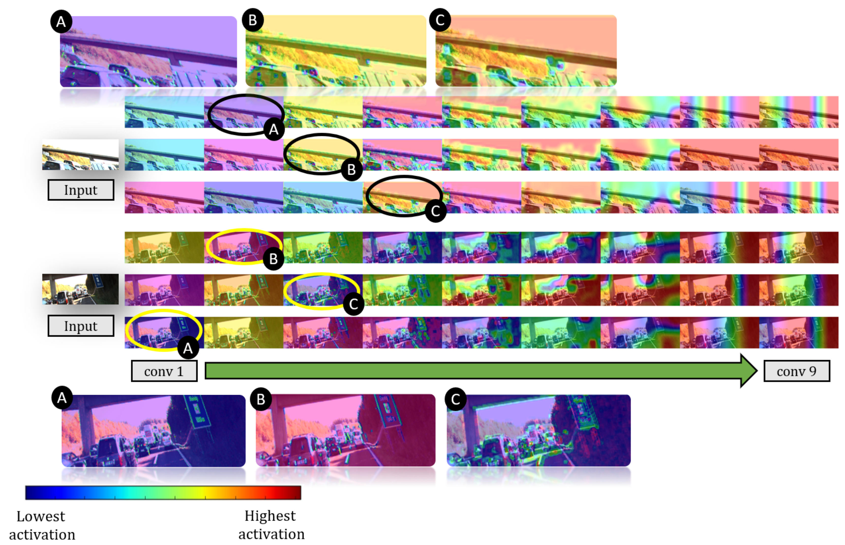
6.3. Activation Visualization
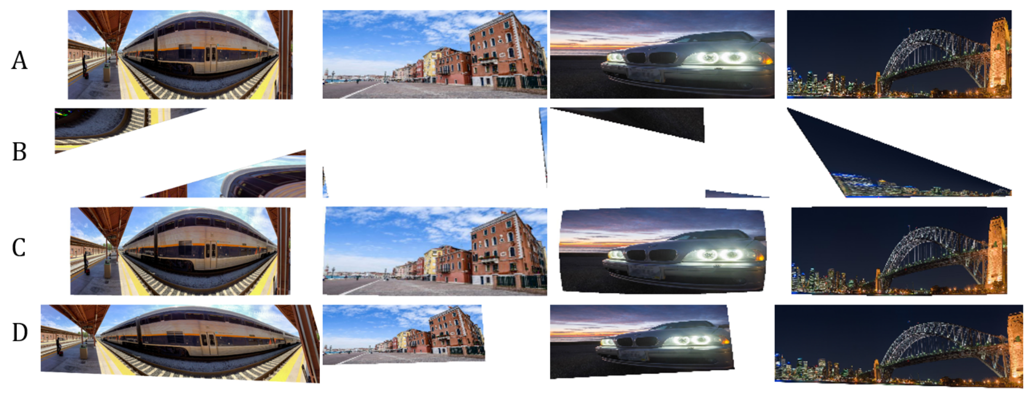
6.4. Model Generalization
6.5. Limitations
7. Conclusions
Author Contributions
Funding
Conflicts of Interest
Appendix A
References
- Sun, H.M. Method of Correcting an Image With Perspective Distortion and Producing an Artificial Image with Perspective Distortion. U.S. Patent 6,947,610, 20 September 2005. [Google Scholar]
- Dobbert, T. Matchmoving: The Invisible Art of Camera Tracking; Serious Skills; Wiley: Hoboken, NJ, USA, 2012. [Google Scholar]
- Carroll, R.; Agarwala, A.; Agrawala, M. Image warps for artistic perspective manipulation. In Proceedings of the ACM SIGGRAPH 2010, Los Angeles, CA, USA, 15–18 December 2010; pp. 1–9. [Google Scholar]
- Chang, C.; Liang, C.; Chuang, Y. Content-aware display adaptation and interactive editing for stereoscopic images. IEEE Trans. Multimed. 2011, 13, 589–601. [Google Scholar] [CrossRef]
- Yang, B.; Jin, J.S.; Li, F.; Han, X.; Tong, W.; Wang, M. A perspective correction method based on the bounding rectangle and least square fitting. In Proceedings of the 2016 13th International Computer Conference on Wavelet Active Media Technology and Information Processing (ICCWAMTIP), Chengdu, China, 16–18 December 2016; pp. 260–264. [Google Scholar] [CrossRef]
- Tan, C.L.; Zhang, L.; Zhang, Z.; Xia, T. Restoring warped document images through 3D shape modeling. IEEE Trans. Pattern Anal. Mach. Intell. 2006, 28, 195–208. [Google Scholar] [CrossRef]
- Ray, L. 2-D and 3-D image registration for medical, remote sensing, and industrial applications. J. Electron. Imaging 2005, 14, 9901. [Google Scholar] [CrossRef]
- Salimans, T.; Goodfellow, I.; Zaremba, W.; Cheung, V.; Radford, A.; Chen, X. Improved techniques for training GANs. In Proceedings of the 30th International Conference on Neural Information Processing Systems, Barcelona, Spain, 5–10 December 2016; Curran Associates Inc.: Red Hook, NY, USA, 2016; pp. 2234–2242. [Google Scholar]
- Srivastava, A.; Valkov, L.; Russell, C.; Gutmann, M.U.; Sutton, C. VEEGAN: Reducing mode collapse in gans using implicit variational learning. In Proceedings of the Advances in Neural Information Processing Systems 30, Long Beach, CA, USA, 4–9 December 2017; Guyon, I., Luxburg, U.V., Bengio, S., Wallach, H., Fergus, R., Vishwanathan, S., Garnett, R., Eds.; Curran Associates, Inc.: Red Hook, NY, USA, 2017; pp. 3308–3318. [Google Scholar]
- Zhao, Y.; Huang, Z.; Li, T.; Chen, W.; Legendre, C.; Ren, X.; Shapiro, A.; Li, H. Learning perspective undistortion of portraits. In Proceedings of the 2019 IEEE/CVF International Conference on Computer Vision (ICCV), Seoul, Korea, 27–28 October 2019. [Google Scholar] [CrossRef] [Green Version]
- Li, X.; Zhang, B.; Sander, P.V.; Liao, J. Blind geometric distortion correction on images through deep learning. In Proceedings of the 2019 IEEE Conference on Computer Vision and Pattern Recognition (CVPR), Long Beach, CA, USA, 15–20 June 2019. [Google Scholar]
- Li, X.; Zhang, B.; Liao, J.; Sander, P.V. Document rectification and illumination correction using a patch-based CNN. ACM Trans. Graph. 2019, 38. [Google Scholar] [CrossRef] [Green Version]
- Hartley, R.; Zisserman, A. Multiple View Geometry in Computer Vision, 2nd ed.; Cambridge University Press: New York, NY, USA, 2003. [Google Scholar]
- Tardif, J.P.; Sturm, P.; Trudeau, M.; Roy, S. Calibration of cameras with radially symmetric distortion. IEEE Trans. Pattern Anal. Mach. Intell. 2008, 31, 1552–1566. [Google Scholar] [CrossRef] [Green Version]
- Tsai, R. A versatile camera calibration technique for high-accuracy 3D machine vision metrology using off-the-shelf TV cameras and lenses. IEEE J. Robot. Autom. 1987, 3, 323–344. [Google Scholar] [CrossRef] [Green Version]
- Vasu, S.; Rajagopalan, A.N.; Seetharaman, G. Camera shutter-independent registration and rectification. IEEE Trans. Image Process. 2017, 27, 1901–1913. [Google Scholar] [CrossRef] [PubMed]
- Lowe, D.G. Distinctive image features from scale-invariant keypoints. Int. J. Comput. Vis. 2004, 60, 91–110. [Google Scholar] [CrossRef]
- Wang, A.; Qiu, T.; Shao, L. A simple method of radial distortion correction with centre of distortion estimation. J. Math. Imaging Vis. 2009, 35, 165–172. [Google Scholar] [CrossRef]
- Bukhari, F.; Dailey, M.N. Automatic radial distortion estimation from a single image. J. Math. Imaging Vis. 2013, 45, 31–45. [Google Scholar] [CrossRef]
- Fitzgibbon, A.W. Simultaneous linear estimation of multiple view geometry and lens distortion. In Proceedings of the 2001 IEEE Computer Society Conference on Computer Vision and Pattern Recognition, Kauai, HI, USA, 8–14 December 2001. [Google Scholar] [CrossRef]
- Chaudhury, K.; DiVerdi, S.; Ioffe, S. Auto-rectification of user photos. In Proceedings of the 2014 IEEE International Conference on Image Processing (ICIP), Paris, France, 27–30 October 2014; pp. 3479–3483. [Google Scholar]
- Santana-Cedrés, D.; Gomez, L.; Alemán-Flores, M.; Salgado, A.; Esclarín, J.; Mazorra, L.; Alvarez, L. Automatic correction of perspective and optical distortions. Comput. Vis. Image Underst. 2017, 161, 1–10. [Google Scholar] [CrossRef]
- Shih, Y.; Lai, W.S.; Liang, C.K. Distortion-free wide-angle portraits on camera phones. ACM Trans. Graph. 2019, 38, 1–12. [Google Scholar] [CrossRef] [Green Version]
- Zhang, Z. A flexible new technique for camera calibration. IEEE Trans. Pattern Anal. Mach. Intell. 2000, 22, 1330–1334. [Google Scholar] [CrossRef] [Green Version]
- Ramalingam, S.; Sturm, P.; Lodha, S.K. Generic self-calibration of central cameras. Comput. Vis. Image Underst. 2010, 114, 210–219. [Google Scholar] [CrossRef]
- Hartley, R.; Kang, S.B. Parameter-free radial distortion correction with center of distortion estimation. IEEE Trans. Pattern Anal. Mach. Intell. 2007, 29, 1309–1321. [Google Scholar] [CrossRef]
- Capel, D.; Zisserman, A. Computer vision applied to super resolution. IEEE Signal Process. Mag. 2003, 20, 75–86. [Google Scholar] [CrossRef] [Green Version]
- Zhang, H.; Carin, L. Multi-shot imaging: Joint alignment, deblurring and resolution-enhancement. In Proceedings of the IEEE Conference on Computer Vision and Pattern Recognition, Columbus, OH, USA, 23–28 June 2014; pp. 2925–2932. [Google Scholar]
- Del Gallego, N.P.; Ilao, J. Multiple-image super-resolution on mobile devices: An image warping approach. EURASIP J. Image Video Process. 2017, 2017, 8. [Google Scholar] [CrossRef] [Green Version]
- Rengarajan, V.; Rajagopalan, A.N.; Aravind, R.; Seetharaman, G. Image registration and change detection under rolling shutter motion blur. IEEE Trans. Pattern Anal. Mach. Intell. 2017, 39, 1959–1972. [Google Scholar] [CrossRef] [PubMed]
- Szeliski, R. Image alignment and stitching: A tutorial. Found. Trends Comput. Graph. Vis. 2007, 2, 1–104. [Google Scholar] [CrossRef]
- Brown, M.; Lowe, D.G. Automatic panoramic image stitching using invariant features. Int. J. Comput. Vis. 2007, 74, 59–73. [Google Scholar] [CrossRef] [Green Version]
- Zhang, F.; Liu, F. Parallax-tolerant image stitching. In Proceedings of the 2014 IEEE Conference on Computer Vision and Pattern Recognition, Columbus, OH, USA, 24–17 June 2014; pp. 3262–3269. [Google Scholar]
- Zomet, A.; Levin, A.; Peleg, S.; Weiss, Y. Seamless image stitching by minimizing false edges. IEEE Trans. Image Process. 2006, 15, 969–977. [Google Scholar] [CrossRef] [PubMed] [Green Version]
- He, K.; Chang, H.; Sun, J. Rectangling panoramic images via warping. ACM Trans. Graph. 2013, 32. [Google Scholar] [CrossRef]
- Shemiakina, J.; Konovalenko, I.; Tropin, D.; Faradjev, I. Fast projective image rectification for planar objects with Manhattan structure. In Proceedings of the Twelfth International Conference on Machine Vision (ICMV 2019), Amsterdam, The Netherlands, 16–18 November 2019; Osten, W., Nikolaev, D.P., Eds.; International Society for Optics and Photonics: Bellingham, WA, USA, 2020; Volume 11433, pp. 450–458. [Google Scholar] [CrossRef] [Green Version]
- Sean, P.; Sangyup, L.; Park, M. Automatic Perspective Control Using Vanishing Points. U.S. Patent 10,354,364, 16 July 2019. [Google Scholar]
- Gallagher, A.C. Using vanishing points to correct camera rotation in images. In Proceedings of the 2nd Canadian Conference on Computer and Robot Vision (CRV’05), Victoria, BC, Canada, 9–11 May 2005; pp. 460–467. [Google Scholar] [CrossRef]
- An, J.; Koo, H.I.; Cho, N.I. Rectification of planar targets using line segments. Mach. Vis. Appl. 2017, 28, 91–100. [Google Scholar] [CrossRef]
- Coughlan, J.M.; Yuille, A.L. The manhattan world assumption: Regularities in scene statistics which enable bayesian inference. In Proceedings of the NIPS 2000, Denver, CO, USA, 1 January 2000. [Google Scholar]
- Lee, H.; Shechtman, E.; Wang, J.; Lee, S. Automatic upright adjustment of photographs. In Proceedings of the 2012 IEEE Conference on Computer Vision and Pattern Recognition, Providence, RI, USA, 18–20 June 2012; pp. 877–884. [Google Scholar] [CrossRef] [Green Version]
- Cai, H.; Jiang, L.; Liu, B.; Deng, Y.; Meng, Q. Assembling convolution neural networks for automatic viewing transformation. IEEE Trans. Ind. Inform. 2019, 16, 587–594. [Google Scholar] [CrossRef]
- Zhai, M.; Workman, S.; Jacobs, N. Detecting vanishing points using global image context in a non-Manhattan world. In Proceedings of the 2016 IEEE Conference on Computer Vision and Pattern Recognition (CVPR), Las Vegas, NV, USA, 26 June–1 July 2016; pp. 5657–5665. [Google Scholar] [CrossRef] [Green Version]
- Das, S.; Mishra, G.; Sudharshana, A.; Shilkrot, R. The common fold: Utilizing the four-fold to dewarp printed documents from a single image. In Proceedings of the 2017 ACM Symposium on Document Engineering, Valletta, Malta, 4–7 September 2017; pp. 125–128. [Google Scholar]
- Das, S.; Ma, K.; Shu, Z.; Samaras, D.; Shilkrot, R. DewarpNet: Single-image document unwarping with stacked 3D and 2D regression networks. In Proceedings of the 2019 IEEE International Conference on Computer Vision (ICCV), Seoul, Korea, 27 October–2 November 2019. [Google Scholar]
- Ma, K.; Shu, Z.; Bai, X.; Wang, J.; Samaras, D. Docunet: Document image unwarping via a stacked U-Net. In Proceedings of the 2018 IEEE Conference on Computer Vision and Pattern Recognition, Salt Lake City, UT, USA, 18–23 June 2018; pp. 4700–4709. [Google Scholar]
- Long, J.; Shelhamer, E.; Darrell, T. Fully convolutional networks for semantic segmentation. In Proceedings of the 2015 IEEE Conference on Computer Vision and Pattern Recognition, Boston, MA, USA, 7–12 June 2015; pp. 3431–3440. [Google Scholar]
- Zhou, B.; Lapedriza, A.; Xiao, J.; Torralba, A.; Oliva, A. Learning deep features for scene recognition using places database. In Proceedings of the Advances in Neural Information Processing Systems 2014, Montreal, QC, Canada, 8–13 December 2014; pp. 487–495. [Google Scholar]
- Geiger, A.; Lenz, P.; Stiller, C.; Urtasun, R. Vision meets Robotics: The KITTI Dataset. Int. J. Robot. Res. 2013, 32, 1231–1237. [Google Scholar] [CrossRef] [Green Version]
- Szeliski, R. Computer Vision: Algorithms and Applications; Springer Science & Business Media: New York, NY, USA, 2010. [Google Scholar]
- Nixon, M.S.; Aguado, A.S. Chapter 4—Low-level feature extraction. In Feature Extraction and Image Processing for Computer Vision, 3rd ed.; Nixon, M.S., Aguado, A.S., Eds.; Academic Press: Oxford, UK, 2012; pp. 137–216. [Google Scholar]
- Huang, G.; Liu, Z.; Van Der Maaten, L.; Weinberger, K.Q. Densely connected convolutional networks. In Proceedings of the 2017 IEEE Conference on Computer Vision and Pattern Recognition (CVPR), Honolulu, HI, USA, 21–26 July 2017; pp. 2261–2269. [Google Scholar]
- Kingma, D.P.; Ba, J. Adam: A method for stochastic optimization. arXiv 2014, arXiv:cs.LG/1412.6980. [Google Scholar]
- Wang, Z.; Simoncelli, E.P.; Bovik, A.C. Multiscale structural similarity for image quality assessment. In Proceedings of the Thrity-Seventh Asilomar Conference on Signals, Systems & Computers, Pacific Grove, CA, USA, 9–12 November 2003; Volume 2, pp. 1398–1402. [Google Scholar]
- Dubrofsky, E. Homography Estimation. In Diplomová Práce; Univerzita Britské Kolumbie: Vancouver, BC, USA, 2009. [Google Scholar]
- Rublee, E.; Rabaud, V.; Konolige, K.; Bradski, G. ORB: An efficient alternative to SIFT or SURF. In Proceedings of the 2011 International Conference on Computer Vision, Barcelona, Spain, 6–13 November 2011; IEEE Computer Society: Washington, DC, USA, 2011; pp. 2564–2571. [Google Scholar] [CrossRef]
- Fischler, M.A.; Bolles, R.C. Random sample consensus: A paradigm for model fitting with applications to image analysis and automated cartography. Commun. ACM 1981, 24, 381–395. [Google Scholar] [CrossRef]
- He, K.; Zhang, X.; Ren, S.; Sun, J. Deep residual learning for image recognition. In Proceedings of the 2016 IEEE Conference on Computer Vision and Pattern Recognition (CVPR), Las Vegas, NV, USA, 27–30 June 2016; pp. 770–778. [Google Scholar]
- Selvaraju, R.R.; Cogswell, M.; Das, A.; Vedantam, R.; Parikh, D.; Batra, D. Grad-CAM: Visual explanations from deep networks via gradient-based localization. Int. J. Comput. Vis. 2019, 128, 336–359. [Google Scholar] [CrossRef] [Green Version]


| Low | High | |
|---|---|---|
| and | ||
| and | ||
| and |
| Method | Transformation Matrix Error | Pixel-Wise Error/Accuracy | ↓ Lower Is Better | |||||
|---|---|---|---|---|---|---|---|---|
| Abs. Rel. ↓ | Sq. Rel. ↓ | RMSE ↓ | Sq.Rel ↓ | RMSE ↓ | SSIM ↑ | Failure Rate ↓ | ||
| Dataset mean | 0.2665 | 0.6895 | 0.5294 | 0.00% | ↑ Higher is better | |||
| Homography estimation | 2.4457 | 3.1937 | 0.1838 | 0.4930 | 0.6781 | 13.90% | ||
| Li et al. [11] | N/A | N/A | N/A | 0.9963 | 0.0253 | 0.00% | ||
| Chaudhury et al. [21] | N/A | N/A | N/A | 0.9975 | 0.0148 | 0.00% | ||
| Ours | 0.0361 | 0.2520 | 0.7981 | 0.00% | ||||
| Pre-Trained Layer | Instances | Parallel? | |
|---|---|---|---|
| Model A | DenseNet | 3 | Yes |
| Model B | ResNet-161 | ||
| Model C | None | ||
| Model D | DenseNet | 1 | No |
| Model | Transformation Matrix Error | Model | Pixel-Wise Error/Accuracy | ↓ Lower Is Better | ||||
|---|---|---|---|---|---|---|---|---|
| Abs. Rel. ↓ | Sq. Rel. ↓ | RMSE ↓ | Sq.Rel ↓ | RMSE ↓ | SSIM ↑ | |||
| Model A | Model A | 0.0361 | 0.2520 | 0.7981 | ↑ Higher is better | |||
| Model B | Model B | 0.0688 | 0.3580 | 0.7562 | ||||
| Model C | Model C | 0.0397 | 0.2707 | 0.7956 | ||||
| Model D | Model D | 0.0577 | 0.3270 | 0.7803 | ||||
| Method | Transformation Matrix Error | Pixel-Wise Error/Accuracy | |||||
|---|---|---|---|---|---|---|---|
| Abs. Rel. ↓ | Sq. Rel. ↓ | RMSE ↓ | Sq.Rel ↓ | RMSE ↓ | SSIM ↓ | ||
| Dataset mean | 0.1054 | 0.5978 | 0.4886 | ↓ Lower is better | |||
| Homography estimation | 1.2790 | 5.4121 | 2.3264 | 0.0968 | 0.4745 | 0.4978 | |
| Li et al. [11] | N/A | N/A | N/A | 0.9969 | 0.0131 | ↑ Higher is better | |
| Chaudhury et al. [21] | N/A | N/A | N/A | 0.9982 | 0.0051 | ||
| Our method | 0.1122 | 0.6339 | 0.6574 | ||||
| Method | Transformation Matrix Error | Pixel-Wise Error/Accuracy | |||||
|---|---|---|---|---|---|---|---|
| Abs. Rel. ↓ | Sq. Rel. ↓ | RMSE ↓ | Sq.Rel ↓ | RMSE ↓ | SSIM ↑ | ||
| Dataset mean | 0.1433 | 0.5641 | 0.5805 | ↓ Lower is better | |||
| Homography estimation | 2.6514 | 3.7950 | 0.1522 | 0.5899 | 0.6178 | ||
| Li et al. [11] | N/A | N/A | N/A | 0.9956 | 0.0169 | ↑Higher is better | |
| Chaudhury et al. [21] | N/A | N/A | N/A | 0.9967 | 0.0096 | ||
| Our method | 0.1355 | 0.5851 | 0.6137 | ||||
© 2020 by the authors. Licensee MDPI, Basel, Switzerland. This article is an open access article distributed under the terms and conditions of the Creative Commons Attribution (CC BY) license (http://creativecommons.org/licenses/by/4.0/).
Share and Cite
Del Gallego, N.P.; Ilao, J.; Cordel, M., II. Blind First-Order Perspective Distortion Correction Using Parallel Convolutional Neural Networks. Sensors 2020, 20, 4898. https://doi.org/10.3390/s20174898
Del Gallego NP, Ilao J, Cordel M II. Blind First-Order Perspective Distortion Correction Using Parallel Convolutional Neural Networks. Sensors. 2020; 20(17):4898. https://doi.org/10.3390/s20174898
Chicago/Turabian StyleDel Gallego, Neil Patrick, Joel Ilao, and Macario Cordel, II. 2020. "Blind First-Order Perspective Distortion Correction Using Parallel Convolutional Neural Networks" Sensors 20, no. 17: 4898. https://doi.org/10.3390/s20174898
APA StyleDel Gallego, N. P., Ilao, J., & Cordel, M., II. (2020). Blind First-Order Perspective Distortion Correction Using Parallel Convolutional Neural Networks. Sensors, 20(17), 4898. https://doi.org/10.3390/s20174898