Low-Power Voltage Transformer Smart Frequency Modeling and Output Prediction up to 2.5 kHz, Using Sinc-Response Approach


Abstract
1. Introduction
2. LPVT Model
3. IR Test Method vs. SR Test Method
3.1. IR Test Method
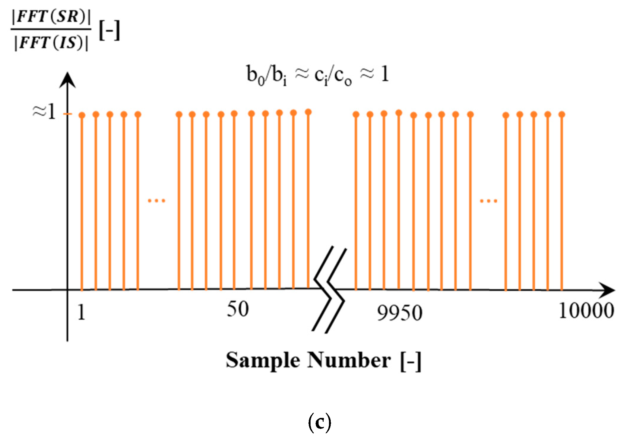
3.2. SR Test Method
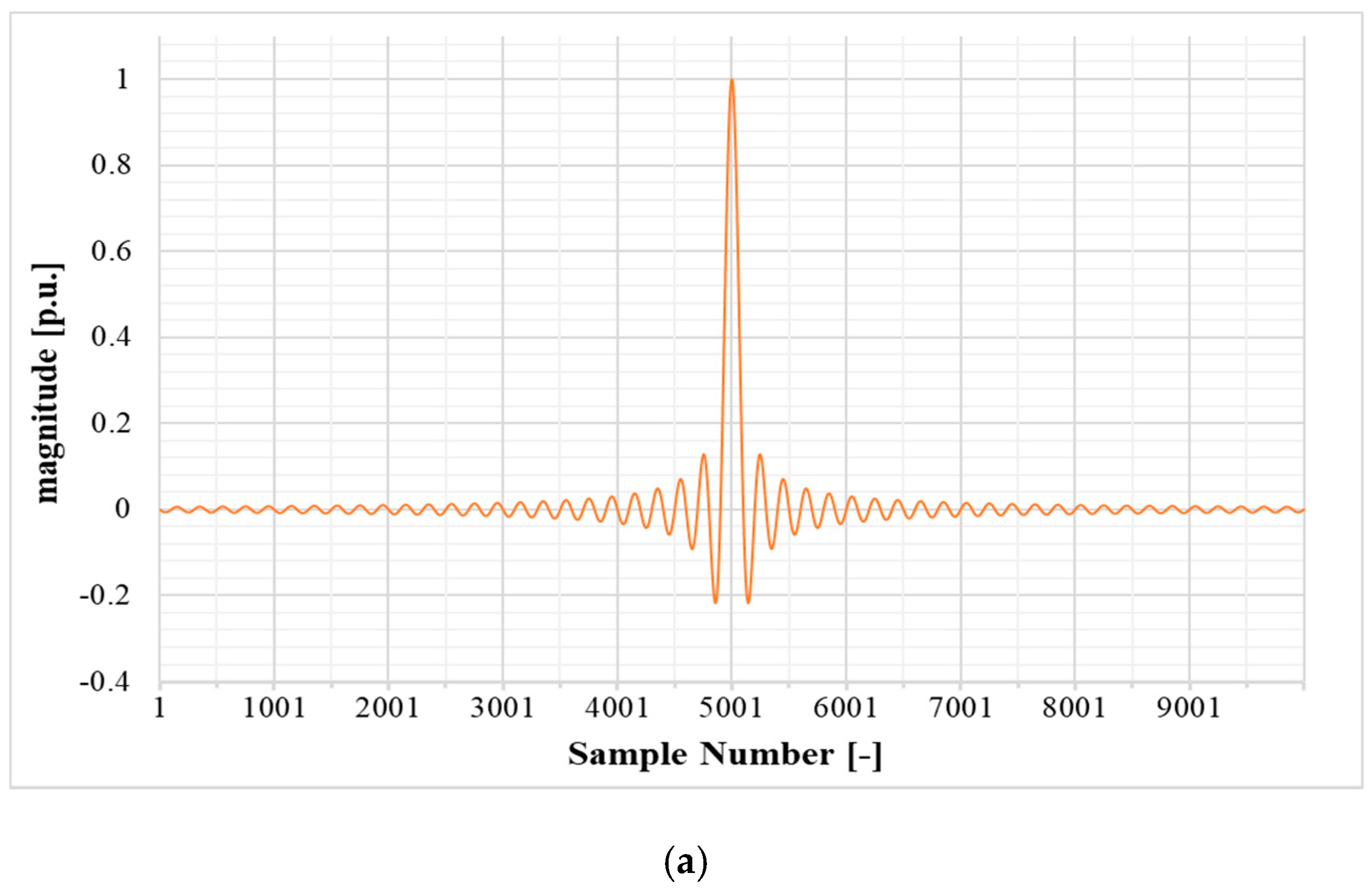
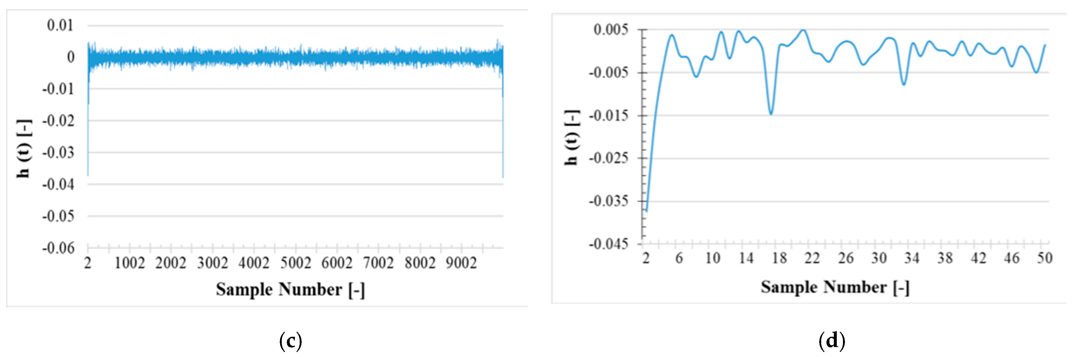
4. Sinc-Signal Design
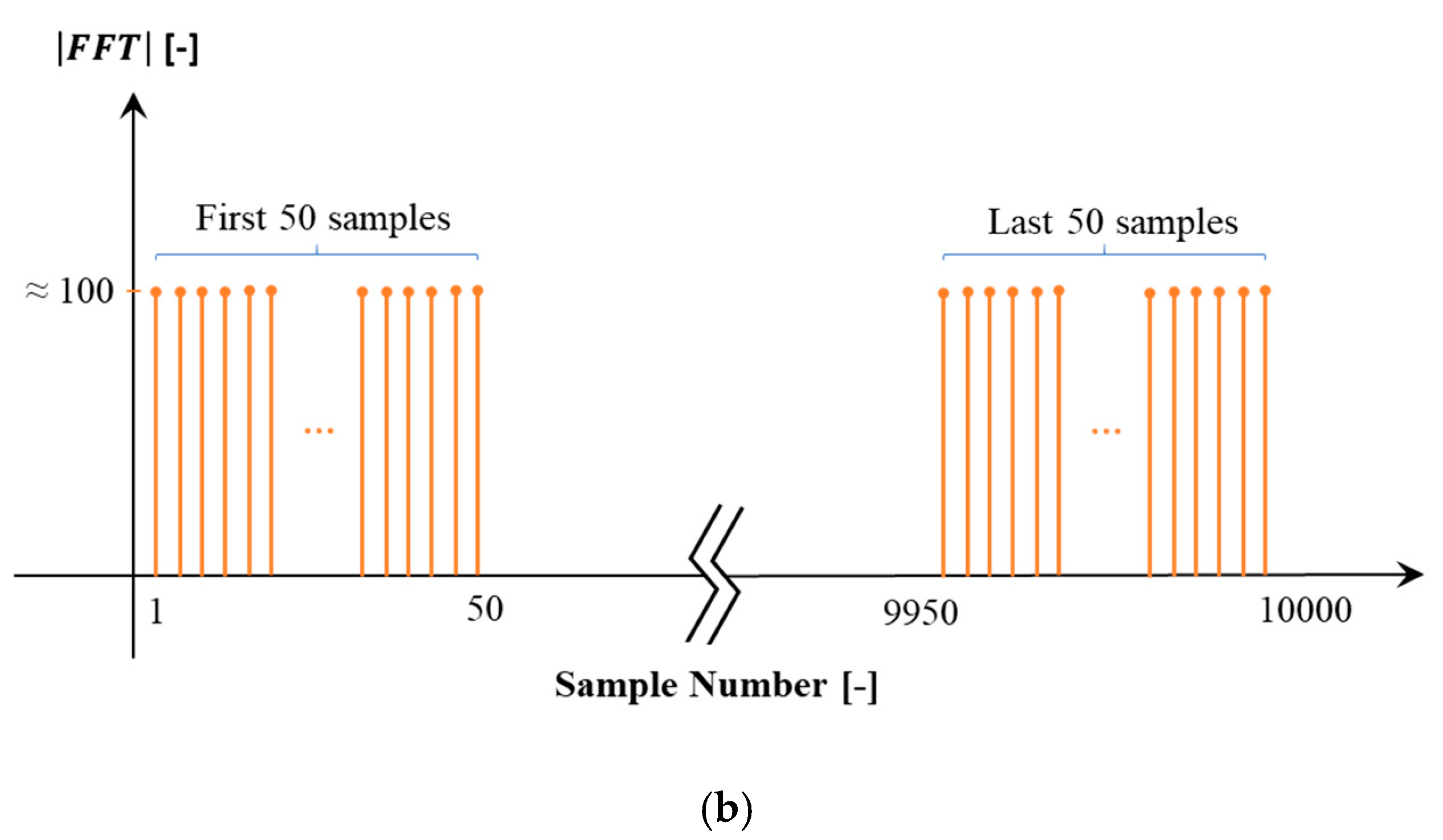
4.1. Sinc Function Fourier-Transform Analysis
- [Hz]: the sinc signal repetition frequency in time domain;
- To [s]: the period of the sinc signal (1/);
- [Sa/s]: sampling frequency of the DAQ;
- [s]: the sampling time (1/);
- N: the number of samples in only one period of the sinc signal.
4.2. Sinc Function Characteristic
4.3. Sinc Function Fourier Series Coefficients
5. Experimental Test Setup
- Agilent 33250A 80 MHz function/arbitrary signal generator used to generate the designed sinc signal;
- Passive capacitive LPVT under test with rated voltage and 0.5 accuracy class;
- Resistive–capacitive reference voltage divider with rated voltage, ratio K and 0.1 accuracy class to measure the primary signal. It is used as a reference;
- NI 9222 data-acquisition board with ±10-V range and 500 kSa/s sampling frequency. Its accuracy features are: ±0.02% gain error and ±0.01% offset error.
6. Experimental Tests
6.1. SR Test Procedure
6.2. SF Test Procedure
6.3. DW Test Procedure
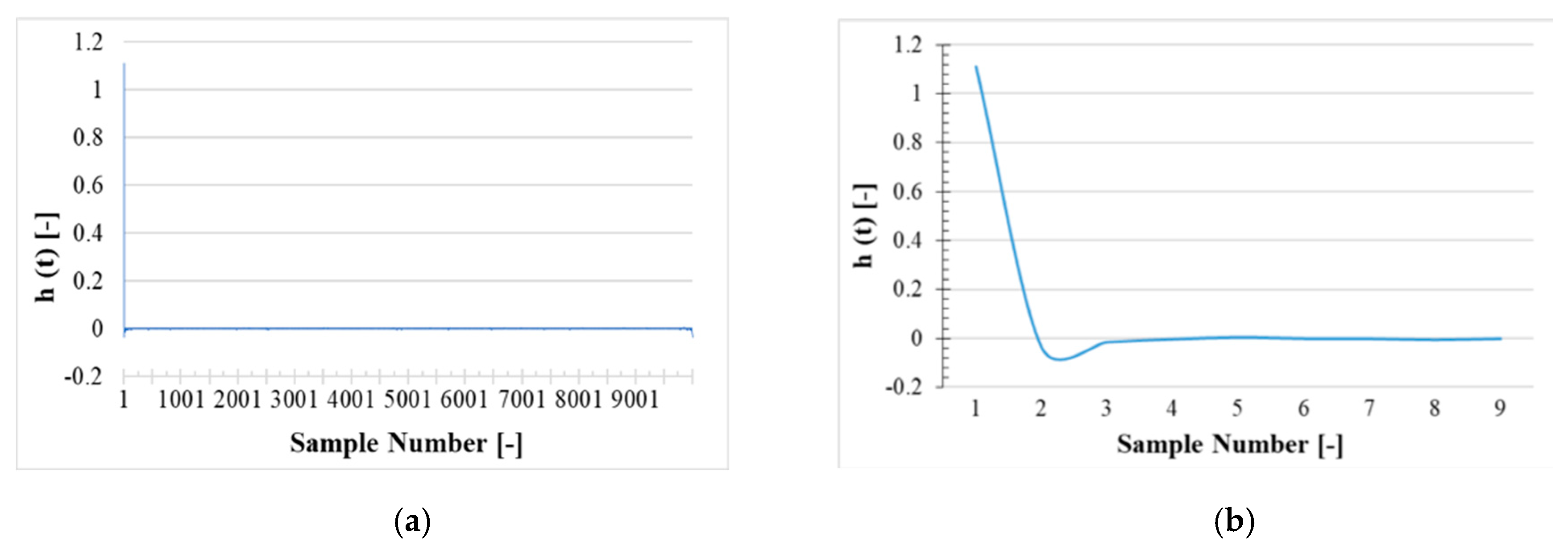
6.4. Output Prediction and Validation
Filtered Transfer Function
7. Results
7.1. SR Experimental Test Results
7.2. Transfer Functions
7.3. SF Experimental Test Results
7.4. DW Experimental Test Results
7.5. Output Prediction and Validation
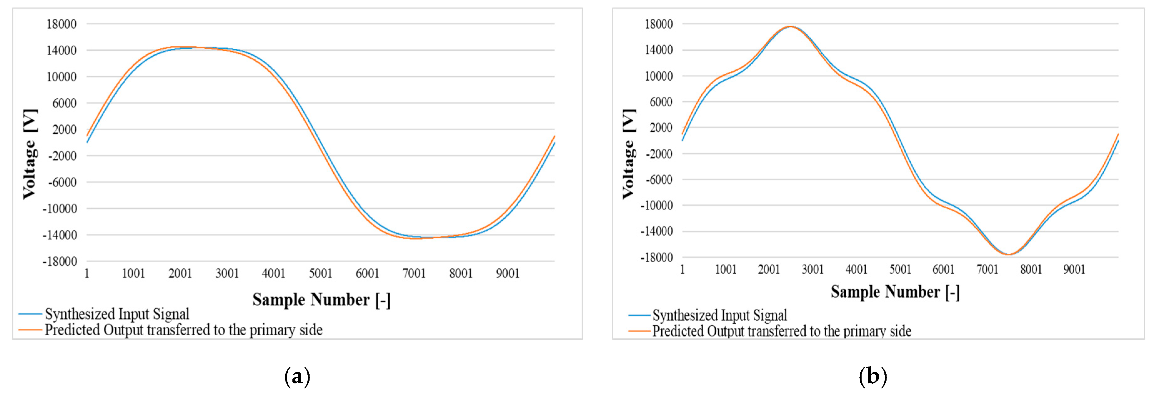
7.5.1. SF Test Prediction
7.5.2. DW Test Prediction
- The SR approach was validated with typical tests methods like SF and DW. By means of and it was demonstrated the high accuracy and validity of the proposed SR test;
- The SR test combined with the mathematical convolution were implemented to estimate the output of the LPVT under test plus its two main accuracy indices: and ;
- All experimental tests were compared with the associated estimated ones demonstrating that, in all cases, the proposed approach provides very accurate results.
8. Conclusions
Author Contributions
Funding
Conflicts of Interest
References
- Crotti, G.; Gallo, D.; Giordano, D.; Landi, C.; Luiso, M. Non-conventional instrument current transformer test set for industrial applications. In Proceedings of the 2014 IEEE International Workshop on Applied Measurements for Power Systems Proceedings (AMPS), Aachen, Germany, 24–26 September 2014; pp. 7–11. [Google Scholar]
- Jiang, H.S.; Yu, X.; Wang, H.J. Electronic current transformer test method research. Appl. Mech. Mater. 2014, 530–531, 310–315. [Google Scholar] [CrossRef]
- Radek, J.; Vaclav, P.; Eddy, D.R.; Stefaan, M. Low-power voltage transformers for use with separable connectors in MV secondary gas-insulated switchgear: New challenge for standardization. Cired Open Access Proc. J. 2017, 2017, 289–292. [Google Scholar]
- Roccato, P.; Sardi, A.; Pasini, G.; Peretto, L.; Tinarelli, R. Traceability of MV low power instrument transformer LPIT. In Proceedings of the 2013 IEEE International Workshop on Applied Measurements for Power Systems, Aachen, Germany, 25–27 September 2013; pp. 13–18. [Google Scholar]
- Kerr, B.; Peretto, L.; Uzelac, N.; Scala, E. Integration challenges of high-accuracy LPIT into MV recloser. Cired-Open Access Proc. J. 2017, 1, 260–263. [Google Scholar] [CrossRef][Green Version]
- Crotti, D.G.; Giordano, C.; Cherbaucich, P. Mazza Calibration of non-conventional instrument transformers. In Proceedings of the Conference on Precision Electromagnetic Measurements, Washington, DC, USA, 1–6 July 2012. [Google Scholar]
- Ren, W.; Yuan, Y.; Hu, X.; Yang, Z.; Zhang, Y. Steady-state error calibration technology for electronic instrument transformer. In Proceedings of the 9th IET International Conference on Advances in Power System Control, Operation and Management (APSCOM 2012), Hong Kong, China, 18–21 November 2012. [Google Scholar]
- Mingotti, A.; Peretto, L.; Tinarelli, R.; Ghaderi, A. Uncertainty Analysis of a Test Bed for Calibrating Voltage Transformers vs. Temperature. Sensors 2019, 19, 4472. [Google Scholar] [CrossRef] [PubMed]
- Mingotti, A.; Peretto, L.; Tinarelli, R.; Ghaderi, A. Uncertainty sources analysis of a calibration system for the accuracy vs. temperature verification of voltage transformers. J. Phys. Conf. Ser. 2018, 1065, 052041. [Google Scholar] [CrossRef]
- Draxler, K.; Styblikova, R. Calibrating an Instrument Voltage Transformer to achieve reduced uncertainty. In Proceedings of the IEEE Instrumentation and Measurement Technology Conference, Singapore, 5–7 May 2009. [Google Scholar]
- Cataliotti, A.; Cosentino, V.; Crotti, G.; Delle Femine, A.; Di Cara, D.; Gallo, D.; Giordano, D.; Landi, C.; Luiso, M.; Modarres, M.; et al. Compensation of Nonlinearity of Voltage and Current Instrument Transformers. IEEE Trans. Instrum. Meas. 2019, 68, 5. [Google Scholar] [CrossRef]
- Močnik, J.; Humar, J.; Žemva, A. A non-conventional instrument transformer. Meas. J. Int. Meas. Confed. 2013, 46, 4114–4120. [Google Scholar] [CrossRef]
- Schmid, J.; Kunde, K. Application of non-conventional voltage and currents sensors in high voltage transmission and distribution systems. In Proceedings of the SMFG 2011-IEEE International Conference on Smart Measurements for Grids, Bologna, Italy, 14–16 November 2011; pp. 64–68. [Google Scholar]
- Wang, H.; Guan, Y.; Feng, S.; Hang, S.; Hu, C. Analysis on the fault of an 110kV independent electronic current transformer. In Proceedings of the 2015 International Conference on Intelligent Transportation, Big Data and Smart City, Halong Bay, Vietnam, 19–20 December 2015; pp. 117–120. [Google Scholar]
- Zhang, H.; Shao, H.; Wang, J. The research on additional errors of voltage transformer connected in series. IEEE Access 2020, 8, 29188–29195. [Google Scholar] [CrossRef]
- IEC 61869-6:2016. Instrument Transformers-Part 6: Additional General Requirements for Low-Power Instrument Transformers; Swiss Standards: Winterthur, Switzerland, 2016.
- Bui, A.T.; Sixdenier, F.; Morel, L.; Burais, N. Characterization and Modeling of a Current Transformer Working Under Thermal Stress. IEEE Trans. Magn. 2012, 10, 2600–2604. [Google Scholar] [CrossRef]
- Nikolić, B.; Khan, S. Modelling and optimisation of design of non-conventional instrument transformers. J. Phys. Conf. Ser. 2019, 1379, 012057. [Google Scholar] [CrossRef]
- Ghaderi, A.; Mingotti, A.; Peretto, L.; Tinarelli, R. Inductive Current Transformer Core Parameters Behaviour vs. Temperature Under Different Working Conditions. Available online: https://www.imeko.org/publications/tc4-2019/IMEKO-TC4-2019-024.pdf (accessed on 28 August 2020).
- Ghaderi, A.; Mingotti, A.; Peretto, L.; Tinarelli, R. Procedure for Ratio Error and Phase Displacement Prediction of Inductive Current Transformers at Different Operating Conditions. In Proceedings of the IEEE International Instrumentation and Measurement Technology Conference (I2MTC), Dubrovnik, Croatia, 25–28 May 2020. [Google Scholar]
- Yan, Y.; Chen, M.; Cheng, Y.; Kong, J.; Ji, H.; Song, A. A Nanosecond High Voltage Impulse Protector for Small Signal Measurement Device. In Proceedings of the Second International Conference on Intelligent System Design and Engineering Application, Sanya, China, 6–7 January 2012. [Google Scholar]
- Shoichiro, S.; Akira, N.; Yoichi, H. Dynamic impulse response model for nonlinear acoustic system and its application to acoustic echo canceller. In Proceedings of the 2012 Second International Conference on Intelligent System Design and Engineering Application, New Paltz, NY, USA, 18–21 October 2009. [Google Scholar]
- Wu, J.J.; Huang, J.J.; Qian, T.; Tang, W.H. Using impulse with appropriate repetition frequency in IFRA test to diagnosis winding deformation in transformer. In Proceedings of the IEEE International Conference on High Voltage Engineering and Application (ICHVE), Chengdu, China, 19–22 September 2016. [Google Scholar]
- Wu, J.J.; Huang, J.J.; Qian, T.; Tang, W.H. Study on Nanosecond Impulse Frequency Response for Detecting Transformer Winding Deformation Based on Morlet Wavelet Transform. In Proceedings of the International Conference on Power System Technology (POWERCON), Guangzhou, China, 6–8 November 2018. [Google Scholar]
- Martin, D.; Tomislav, Ž.; Gabrijel, K. Finite-Impulse-Response Modeling of Voltage Instrument Transformers Applicable for Fast Front Transients Simulations. J. Energy 2018, 67, 8–14. [Google Scholar]
- Lamedica, R.; Pompili, M.; Cauzillo, B.A.; Sangiovanni, S.; Calcara, L.; Ruvio, A. Instrument Voltage Transformer time-response to fast impulse. In Proceedings of the 17th International Conference on Harmonics and Quality of Power (ICHQP), Belo Horizonte, Brazil, 16–19 October 2016. [Google Scholar]
- Buchhagen, C.; Fischer, M.; Hofmann, L.; Däumling, H. Metrological determination of the frequency response of inductive voltage transformers up to 20 kHz. In Proceedings of the IEEE Power & Energy Society General Meeting, Vancouver, BC, Canada, 21–25 July 2013. [Google Scholar]
- Seljeseth, H.; Saethre, E.A.; Ohnstad, T.; Lien, I. Voltage transformer frequency response. Measuring harmonics in Norwegian 300 kV and 132 kV power systems. In Proceedings of the 8th International Conference on Harmonics and Quality of Power, Athens, Greece, 14–16 October 1998. [Google Scholar]
- Klatt, M.; Meyer, J.; Elst, M.; Schegner, P. Frequency Responses of MV voltage transformers in the range of 50 Hz to 10 kHz. In Proceedings of the 14th International Conference on Harmonics and Quality of Power—ICHQP 2010, Bergamo, Italy, 26–29 September 2010. [Google Scholar]
- Zhao, S.; Li, H.; Crossley, P.; Ghassemi, F. Test and analysis of harmonic responses of high voltage instrument voltage transformers. In Proceedings of the 12th IET International Conference on Developments in Power System Protection (DPSP 2014), Copenhagen, Denmark, 31 March–3 April 2014. [Google Scholar]
- Kaczmarek, M.; Brodecki, D.; Nowicz, R. Analysis of operation of voltage transformers during interruptions and dips of primary voltage. In Proceedings of the 10th International Conference on Electrical Power Quality and Utilisation, Lodz, Poland, 15–17 September 2009. [Google Scholar]
- Liu, Y.; Lin, F.; Zhang, Q.; Zhong, H. Design and construction of a rogowski coil for measuring wide pulsed current. IEEE Sens. J. 2010, 11, 123–130. [Google Scholar] [CrossRef]
- Yang, Q.; Su, P.; Chen, Y. Comparison of Impulse Wave and Sweep Frequency Response Analysis Methods for Diagnosis of Transformer Winding Faults. Energies 2017, 10, 431. [Google Scholar] [CrossRef]
- Gómez, P.; De León, F.; Hernández, I.A. Impulse-Response Analysis of Toroidal Core Distribution Transformers for Dielectric Design. Available online: http://engineering.nyu.edu/power/sites/engineering.nyu.edu.power/files/uploads/Impulse-Response%20Analysis%20of%20Toroidal%20Core%20Distribution%20Transformers%20for%20Dielectric%20Design.pdf (accessed on 28 August 2020).
- Mingotti, A.; Peretto, L.; Tinarelli, R. Smart Characterization of Rogowski Coils by Using a Synthetized Signal. Sensors 2020, 20, 3359. [Google Scholar] [CrossRef] [PubMed]
- Trek Model 20/20C-HSHigh-Speed High-Voltage Power Amplifier. Available online: http://www.trekinc.com/pdf/20-20C-HSSales.pdf (accessed on 28 August 2020).


| Output Voltage Range | 0 to 20–kV DC or AC Peak | DC Voltage Gain | 20,000 V/1 V |
|---|---|---|---|
| Input voltage range | 0 to 10–V DC or AC peak | Drift with time | <50 ppm/h |
| DC voltage gain accuracy | <0.1% of full scale | Slew rate | 800 V/µs |
| Drift with temperature | <100 ppm/°C | Signal bandwidth | DC to 5.2 kHz |
| f (Hz) | ε (%) | Δφ (rad) | ||
|---|---|---|---|---|
| Mean Value | Mean Value | |||
| 50 | 0.015 | 0.02 | 0.0647 | 0.0001 |
| 150 (3rd harmonic) | 0.28 | 0.01 | 0.0187 | 0.0001 |
| 250 (5th harmonic) | 0.246 | 0.009 | 0.00947 | 0.00009 |
| 350 (7th harmonic) | 0.212 | 0.008 | 0.00548 | 0.00008 |
| 500 | 0.166 | 0.008 | 0.00244 | 0.00008 |
| 1000 | 0.069 | 0.007 | 0.00115 | 0.00007 |
| f (Hz) | ε (%) | Δφ (rad) | ||
|---|---|---|---|---|
| Mean Value | Mean Value | |||
| 50 | 0.1435 | 0.0002 | 0.064691 | 0.000002 |
| 500 | 0.1638 | 0.0002 | 0.002444 | 0.000002 |
| 1000 | 0.0761 | 0.0002 | 0.001190 | 0.000002 |
| Test | Component | ε (%) | Δφ (rad) | ||
|---|---|---|---|---|---|
| Mean Value | Mean Value | ||||
| 50 Hz + 3rd | 50 Hz | 0.1475 | 0.0002 | 0.064736 | 0.000001 |
| 150 Hz | 0.3103 | 0.0008 | 0.018602 | 0.000008 | |
| 50 Hz + 5th | 50 Hz | 0.1396 | 0.0001 | 0.064723 | 0.000001 |
| 250 Hz | 0.2692 | 0.0007 | 0.009485 | 0.000007 | |
| 50 Hz + 7th | 50 Hz | 0.1406 | 0.0002 | 0.064721 | 0.000001 |
| 350 Hz | 0.2327 | 0.0006 | 0.005461 | 0.000006 | |
| 50 Hz + all | 50 Hz | 0.1409 | 0.0001 | 0.064719 | 0.000001 |
| 150 Hz | 0.3083 | 0.0008 | 0.01857 | 0.00001 | |
| 250 Hz | 0.2691 | 0.0008 | 0.009433 | 0.000007 | |
| 350 Hz | 0.2302 | 0.0007 | 0.005462 | 0.000007 | |
| f (Hz) | SR Experimental Test Results | SF Prediction Results by Simulation | ||
|---|---|---|---|---|
| ε (%) | Δφ (rad) | (%) | (rad) | |
| 50 | 0.15 | 0.0647 | 0.15 | 0.0647 |
| 500 | 0.166 | 0.00244 | 0.166 | 0.00244 |
| 1000 | 0.069 | −0.00115 | 0.069 | −0.00115 |
| Test | Component | ||
|---|---|---|---|
| 50 Hz + 3rd | 50 Hz | 0.15 | 0.0647 |
| 150 Hz | 0.28 | 0.0187 | |
| 50 Hz + 5th | 50 Hz | 0.15 | 0.0647 |
| 250 Hz | 0.246 | 0.00947 | |
| 50 Hz + 7th | 50 Hz | 0.15 | 0.0647 |
| 350 Hz | 0.212 | 0.00548 | |
| 50 Hz + all | 50 Hz | 0.15 | 0.0647 |
| 150 Hz | 0.28 | 0.0187 | |
| 250 Hz | 0.246 | 0.00947 | |
| 350 Hz | 0.212 | 0.00548 |
© 2020 by the authors. Licensee MDPI, Basel, Switzerland. This article is an open access article distributed under the terms and conditions of the Creative Commons Attribution (CC BY) license (http://creativecommons.org/licenses/by/4.0/).
Share and Cite
Ghaderi, A.; Mingotti, A.; Peretto, L.; Tinarelli, R. Low-Power Voltage Transformer Smart Frequency Modeling and Output Prediction up to 2.5 kHz, Using Sinc-Response Approach. Sensors 2020, 20, 4889. https://doi.org/10.3390/s20174889
Ghaderi A, Mingotti A, Peretto L, Tinarelli R. Low-Power Voltage Transformer Smart Frequency Modeling and Output Prediction up to 2.5 kHz, Using Sinc-Response Approach. Sensors. 2020; 20(17):4889. https://doi.org/10.3390/s20174889
Chicago/Turabian StyleGhaderi, Abbas, Alessandro Mingotti, Lorenzo Peretto, and Roberto Tinarelli. 2020. "Low-Power Voltage Transformer Smart Frequency Modeling and Output Prediction up to 2.5 kHz, Using Sinc-Response Approach" Sensors 20, no. 17: 4889. https://doi.org/10.3390/s20174889
APA StyleGhaderi, A., Mingotti, A., Peretto, L., & Tinarelli, R. (2020). Low-Power Voltage Transformer Smart Frequency Modeling and Output Prediction up to 2.5 kHz, Using Sinc-Response Approach. Sensors, 20(17), 4889. https://doi.org/10.3390/s20174889