A Grey Model and Mixture Gaussian Residual Analysis-Based Position Estimator in an Indoor Environment


Abstract
1. Introduction
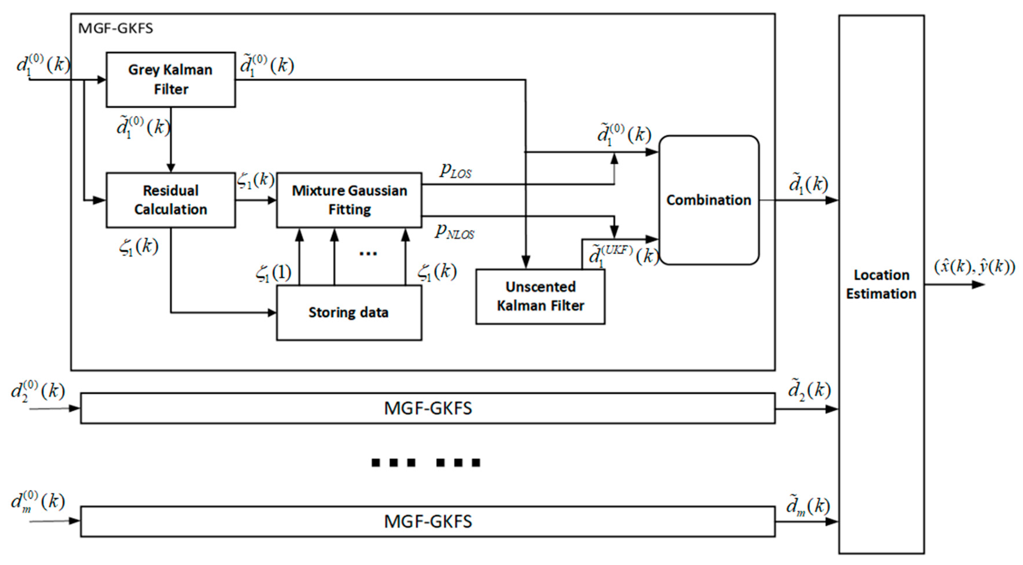
- GKF is proposed to pre-process the measured distance. It could mitigate the process noise caused by target random moving speed and direction. If the propagation path is NLOS, the adverse distance measurement error interference can also be effectively alleviated. After pre-processing, the localization accuracy significantly improves the IMM algorithm.
- Since GKF greatly reduces noise interference, the residual could be calculated by subtracting the pre-processed value from measurement, which is closer to the true measurement error.
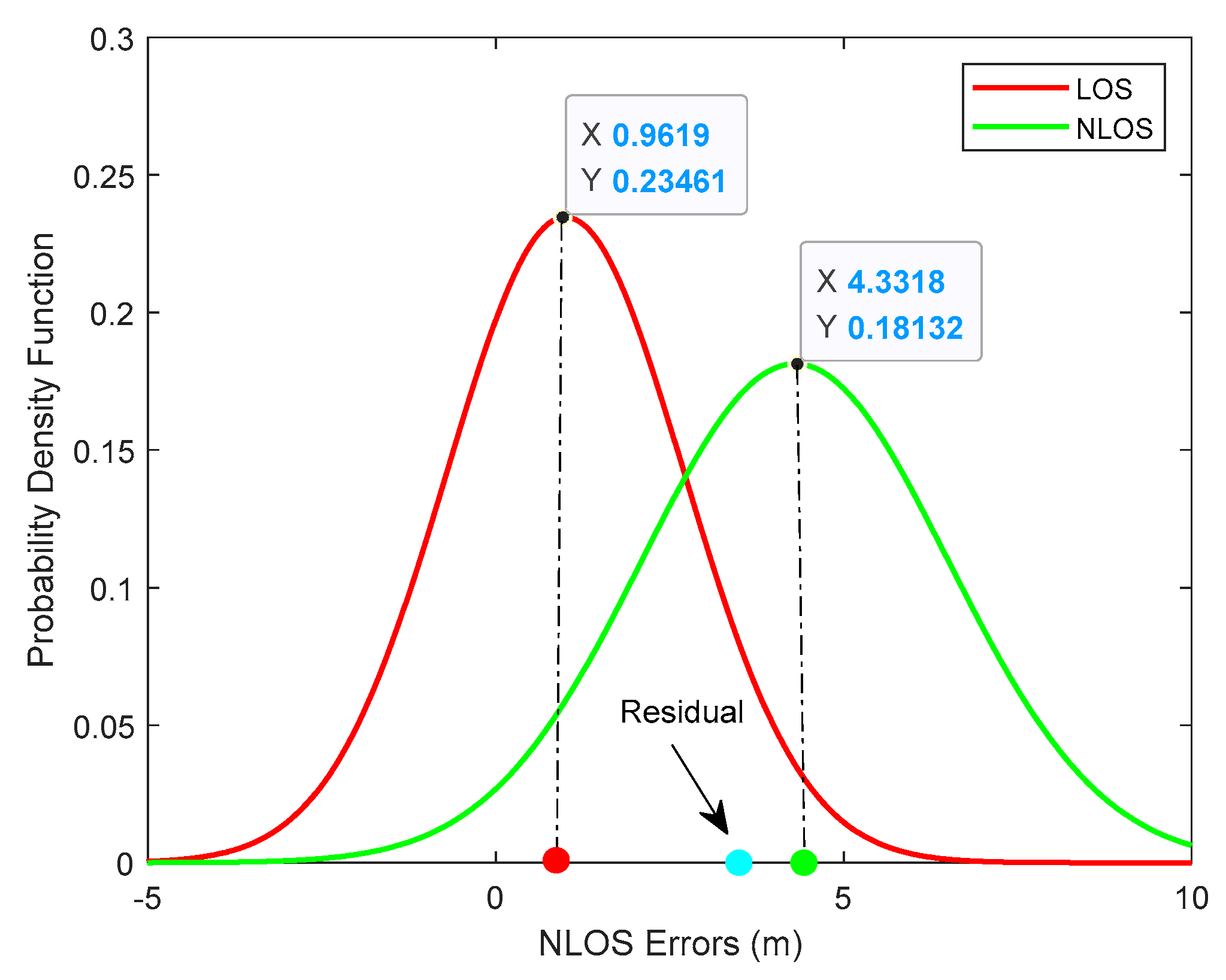
- A soft NLOS identification method is proposed to give the probability of conditions based on residual analysis. Only one measurement needs to be done at a certain time step, instead of taking multiple measurements in a traditional probabilistic weighting algorithm based on a Gaussian mixture model (GMM) [11].
- We adopt a TOA ranging method based on UWB in 2D scenario. The proposed algorithm could apply to other range-based localization model such as RSS and AOA. The entire algorithm is not supported by any priori knowledge.
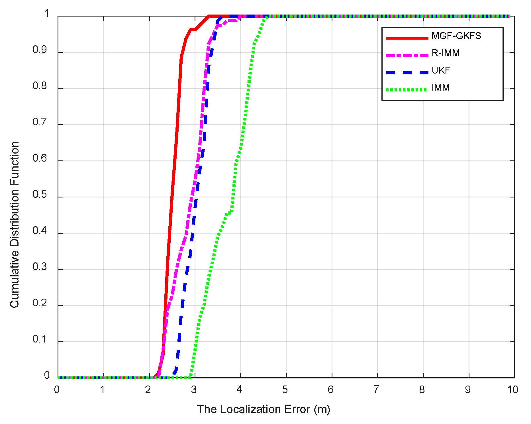
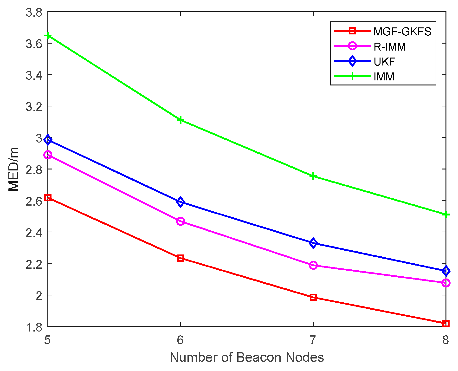
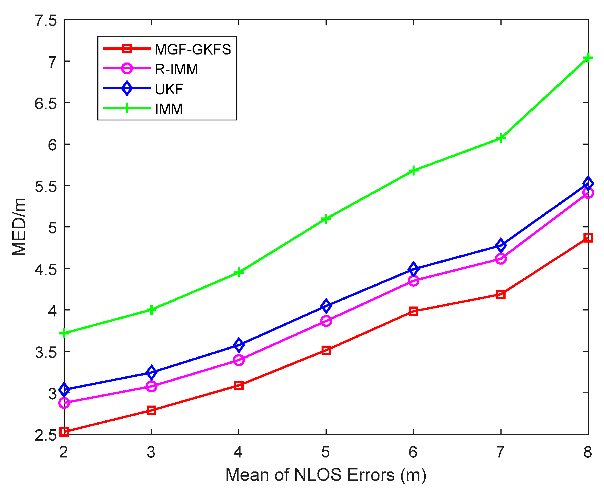
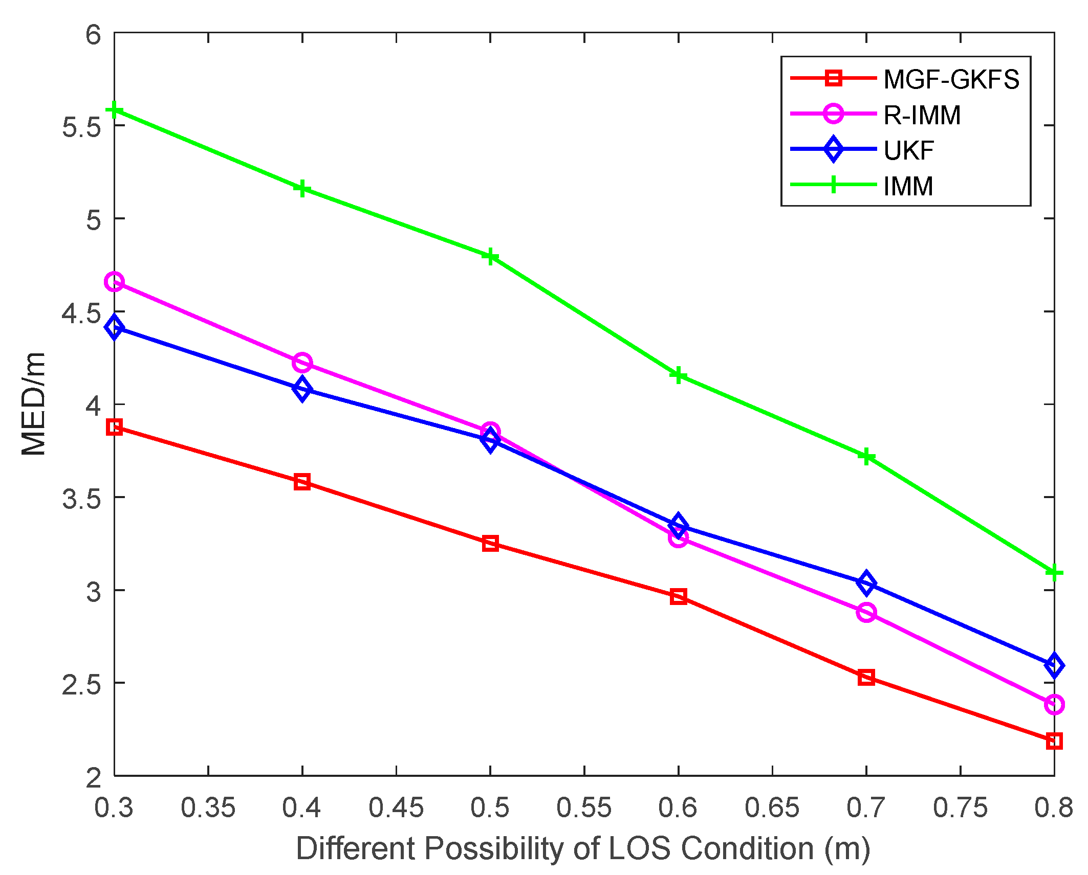
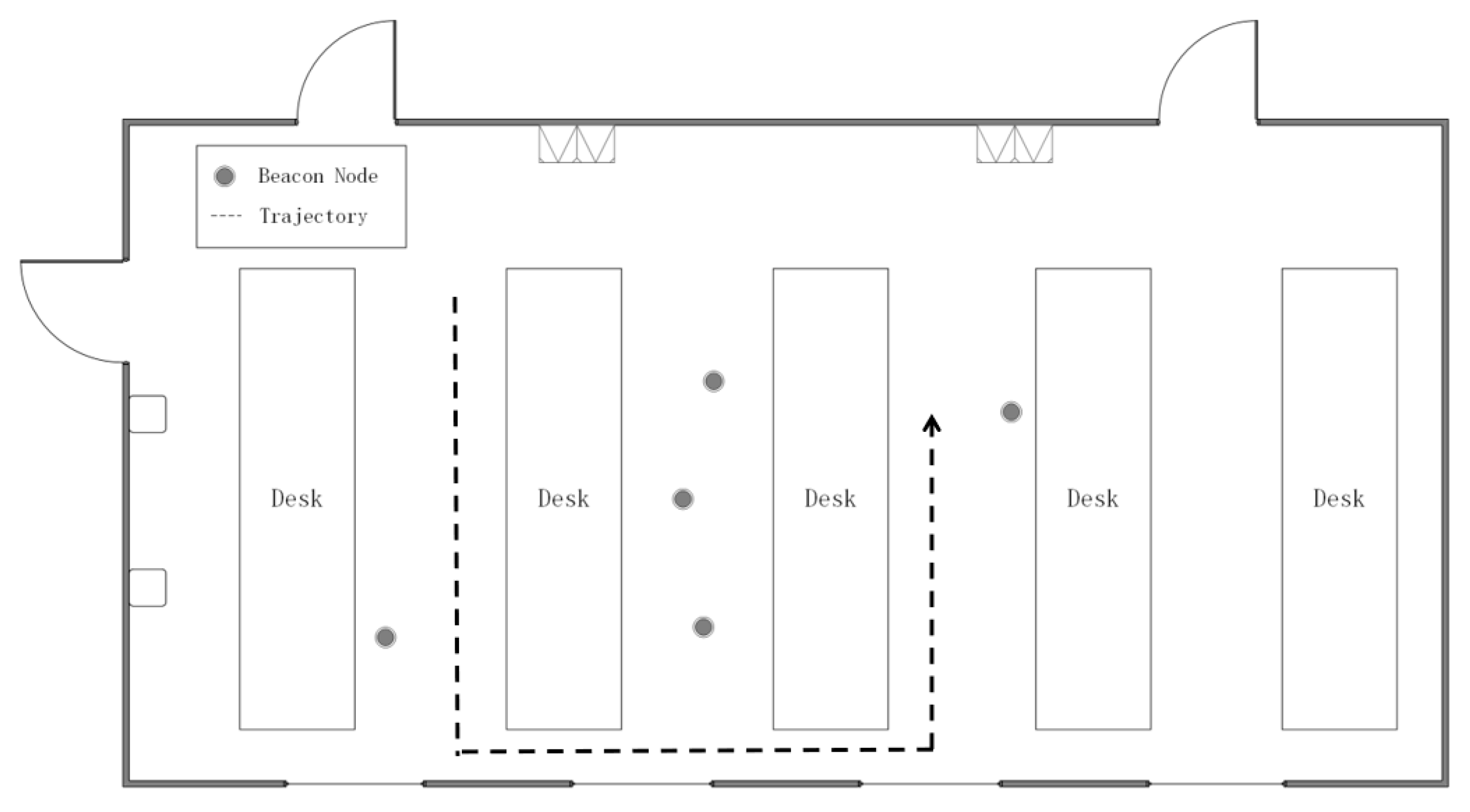
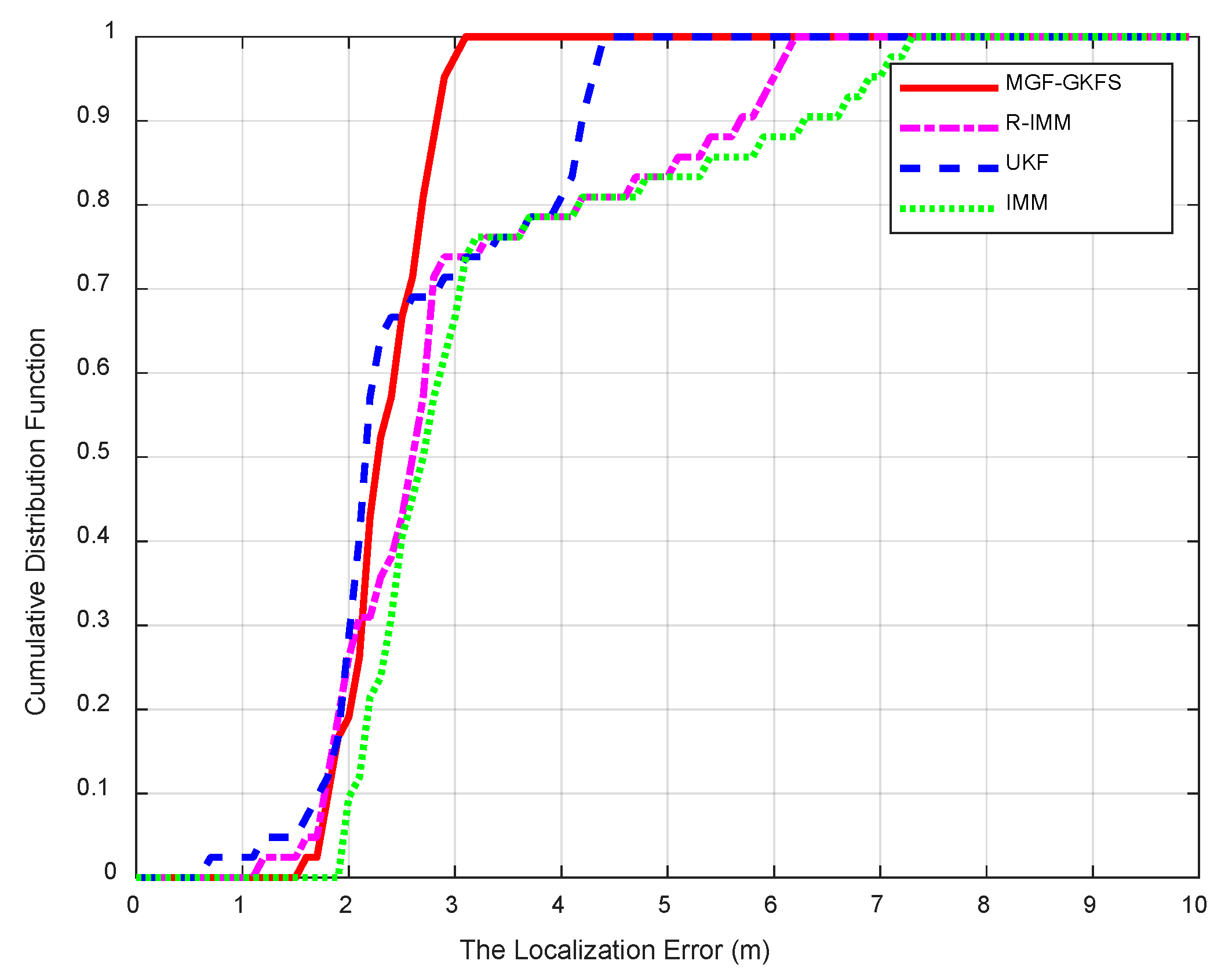
- Full-scale simulations and experiments are conducted to validate the robustness of our algorithm under various NLOS distributions. An actual scenario experiment proves good performance compared to R-IMM, unscented Kalman filter (UKF) and interacting multiple model (IMM).
- MGF-GKFS is based on the distance filtering so it can be easily extended to 3D scenes.
2. Notations
3. Related Works
4. Background
4.1. Signal Model
4.2. A Brief Introduction to the Gaussian Mixture Model (GMM)
5. Proposed Method
5.1. General Concept
5.1.1. The State Equation
5.1.2. The Measurement Equation
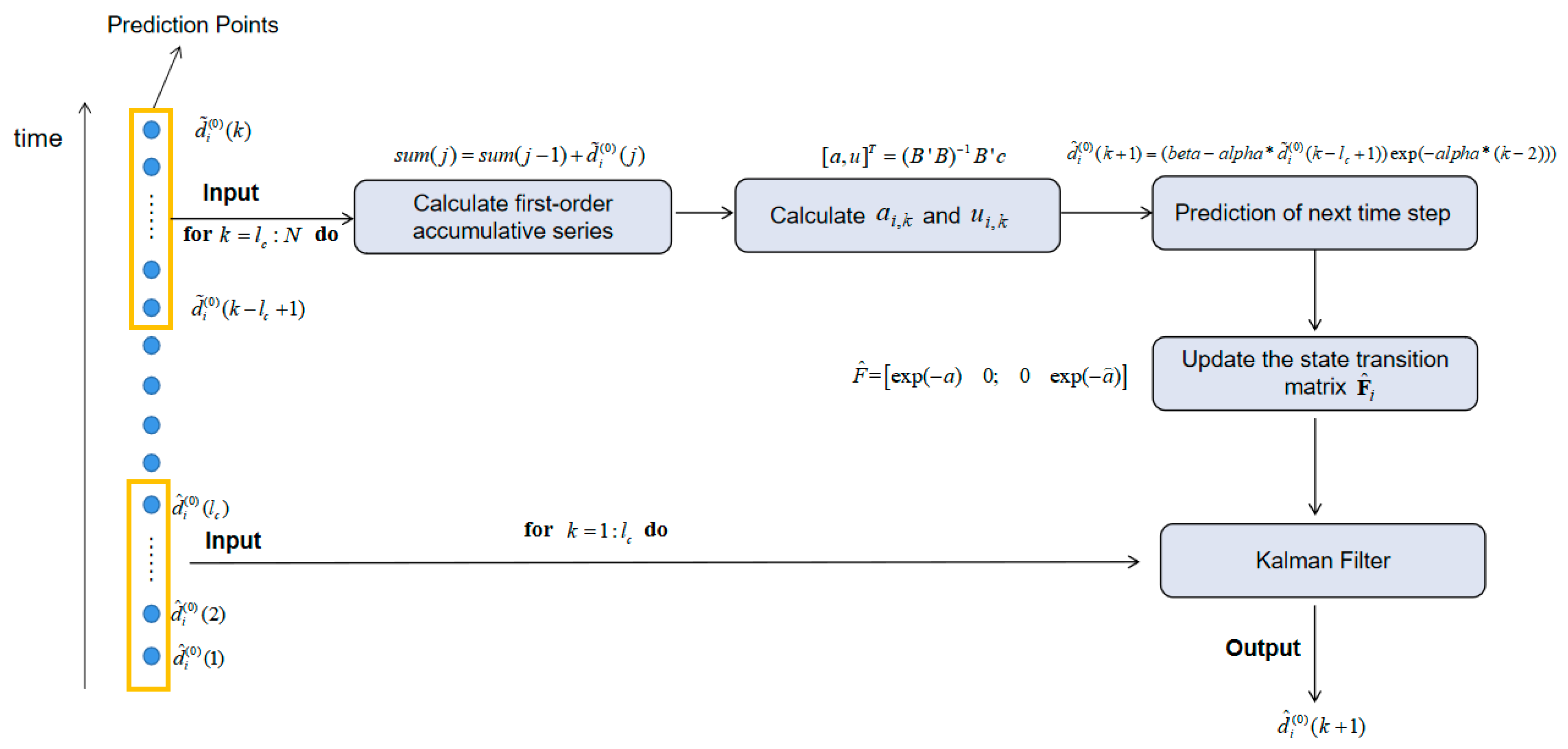
5.2. Grey Kalman Filter (GKF)
| Algorithm 1. The pre-processing for the measurements based on grey Kalman filter (GKF) |
| Input: |
| Output: |
| begin |
| fori = 1: M do |
| for do |
| for j= do |
| end for |
| end for |
| for do |
| end for |
| end for |
| end |
5.3. Mixture Gaussian Fitting (MGF)
- E-step. Calculate the probability that the residual value belongs to the j-th Gaussian distribution as Equation (38).
- M-step. Calculate the partial derivative of the Equation (36) and let the derivative function equal to zero. Solve unknown parameters of Gaussian distribution as Equations (39)–(41).
| Algorithm 2. Pseudocode of mixture Gaussian fitting (MGF) |
| Input: |
| Output: |
| begin |
| fordo |
| for do |
| end for |
| end for |
| end |
5.4. Unscented Kalman Filter (UKF)
5.5. Data Fusion and Position Estimation
6. Simulation and Experiment Results
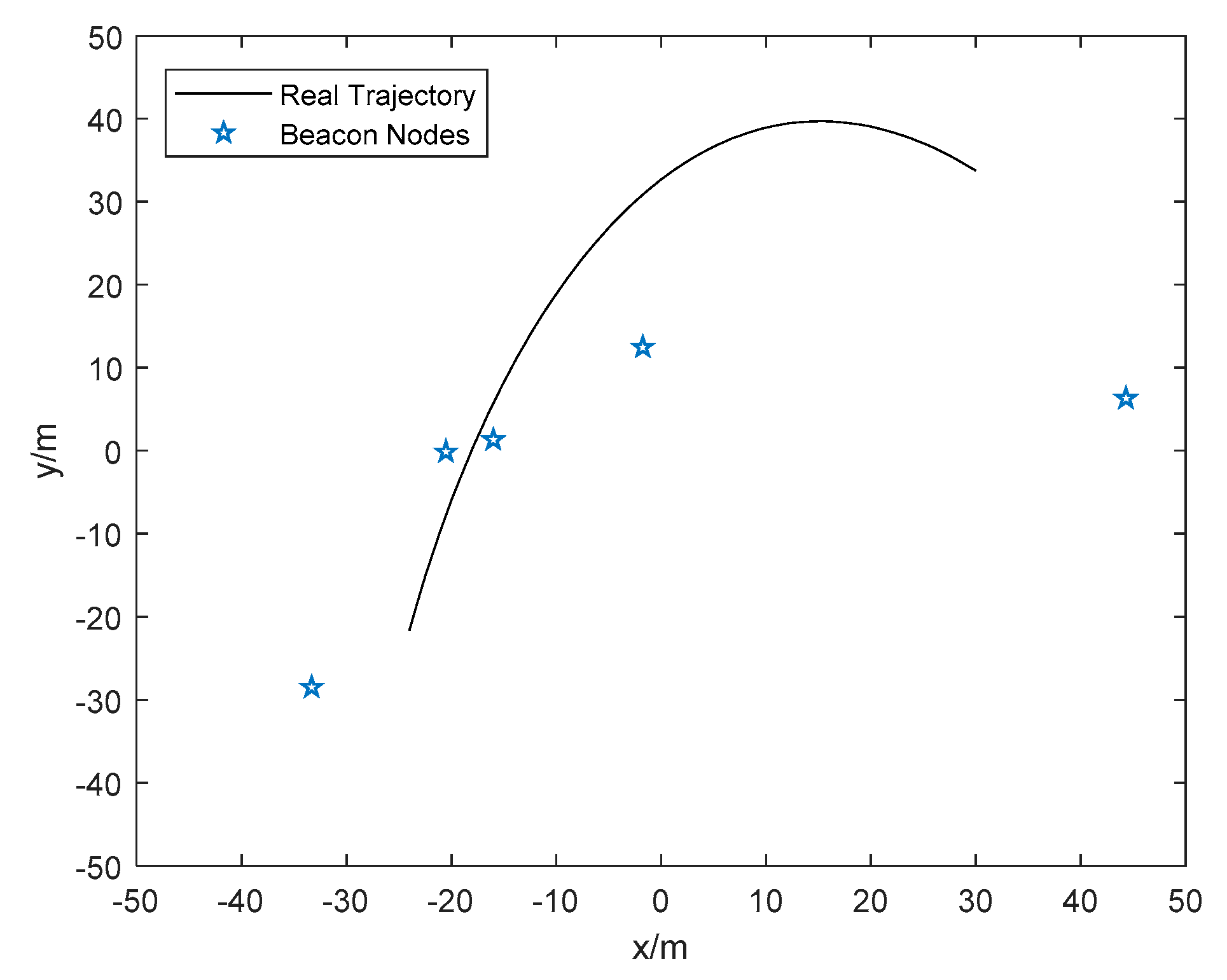
6.1. Simulation Results
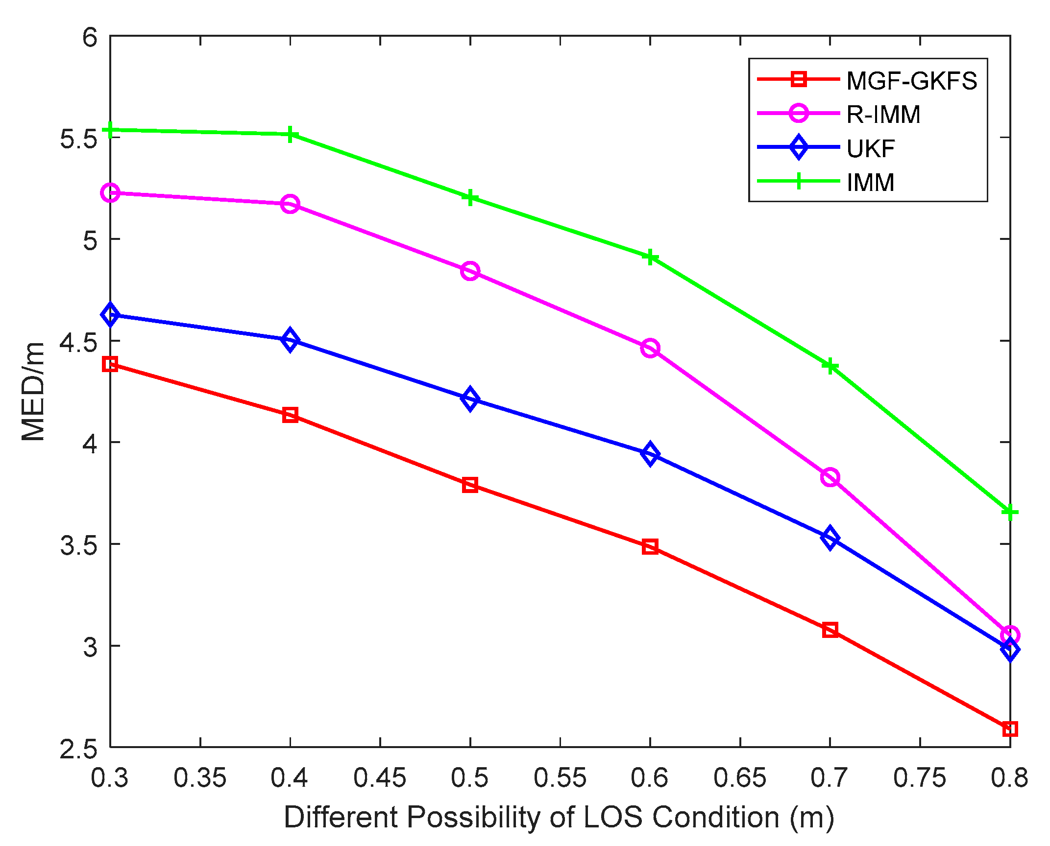
6.1.1. Gaussian Distribution
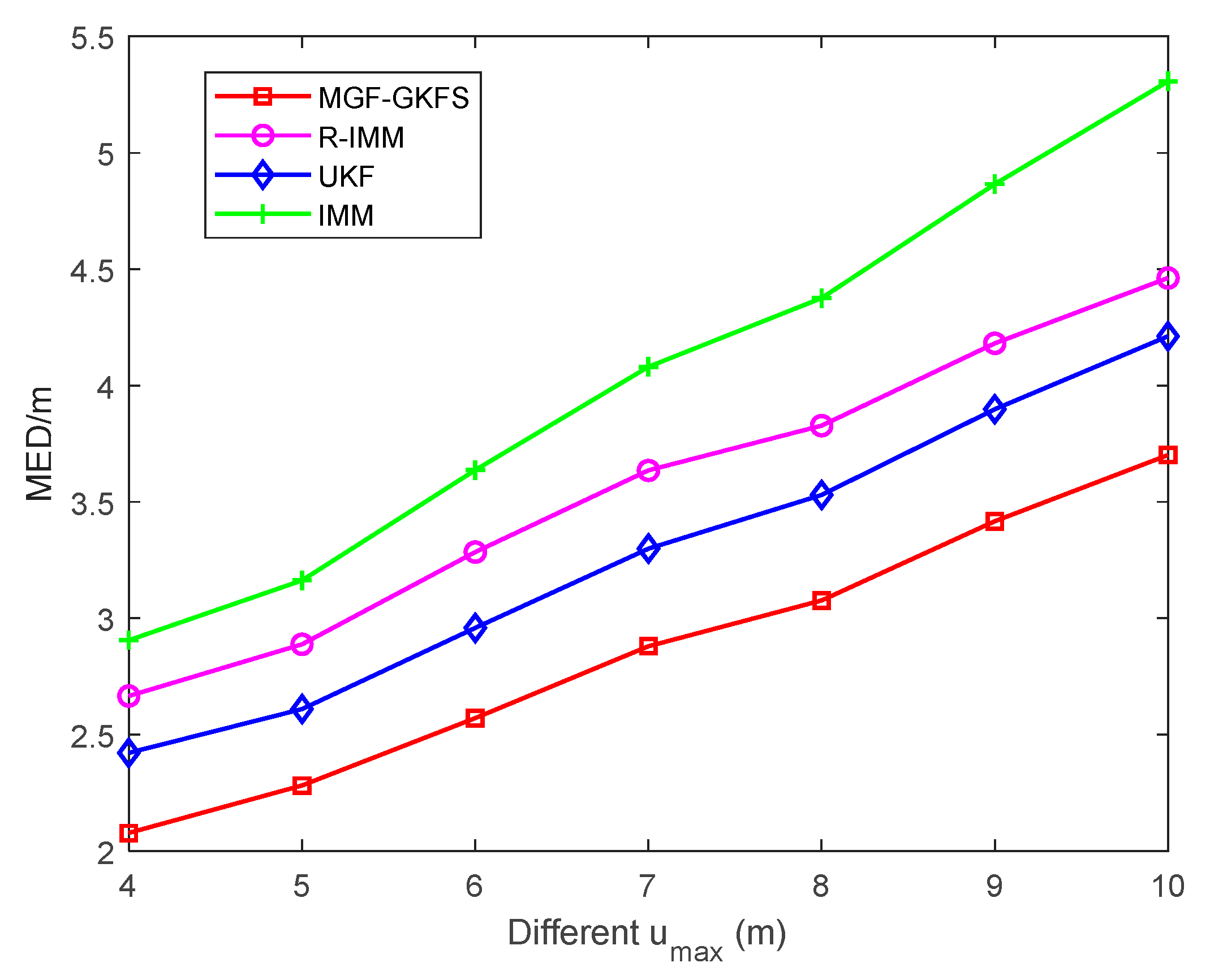
6.1.2. Uniform Distribution
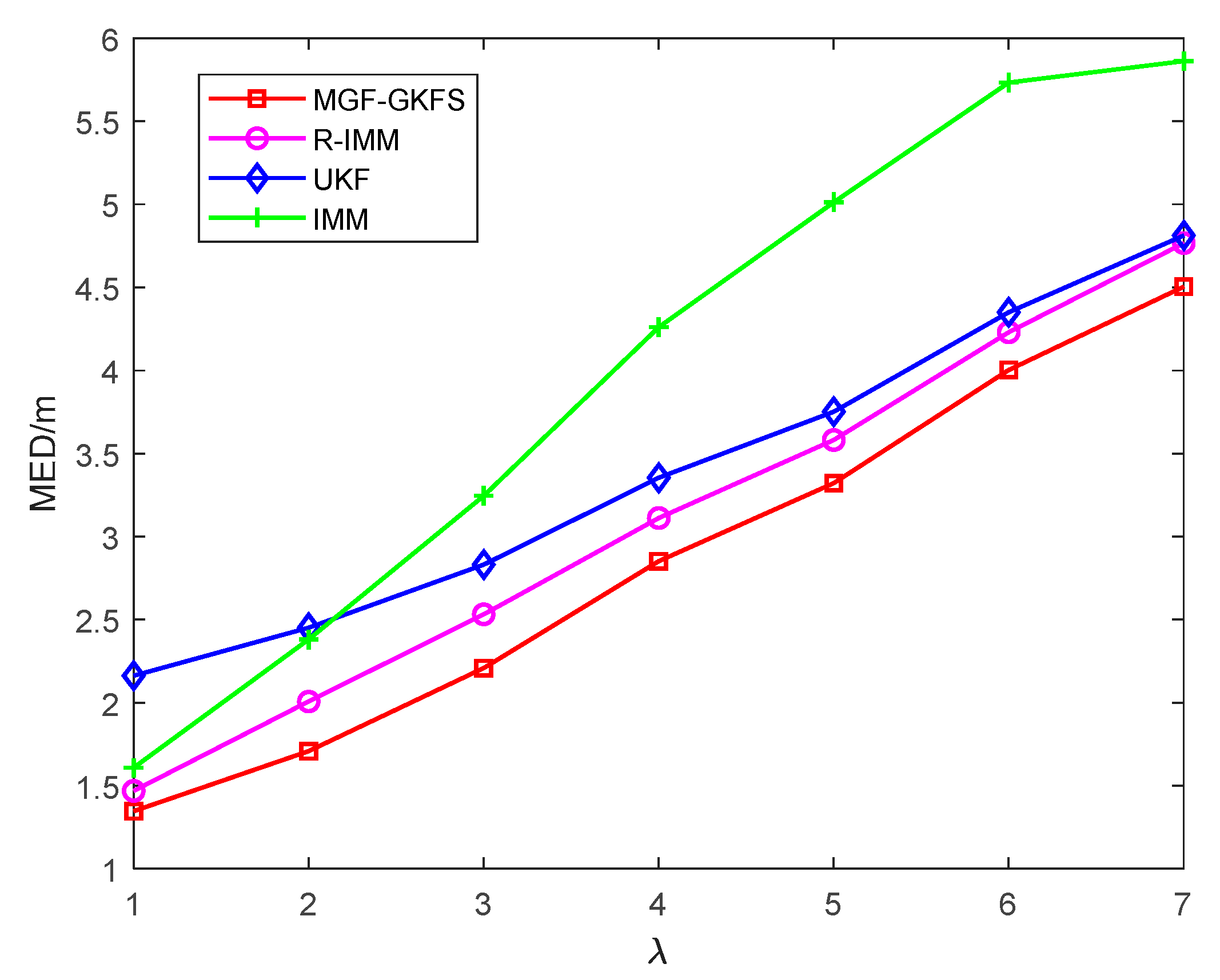
6.1.3. Exponential Distribution
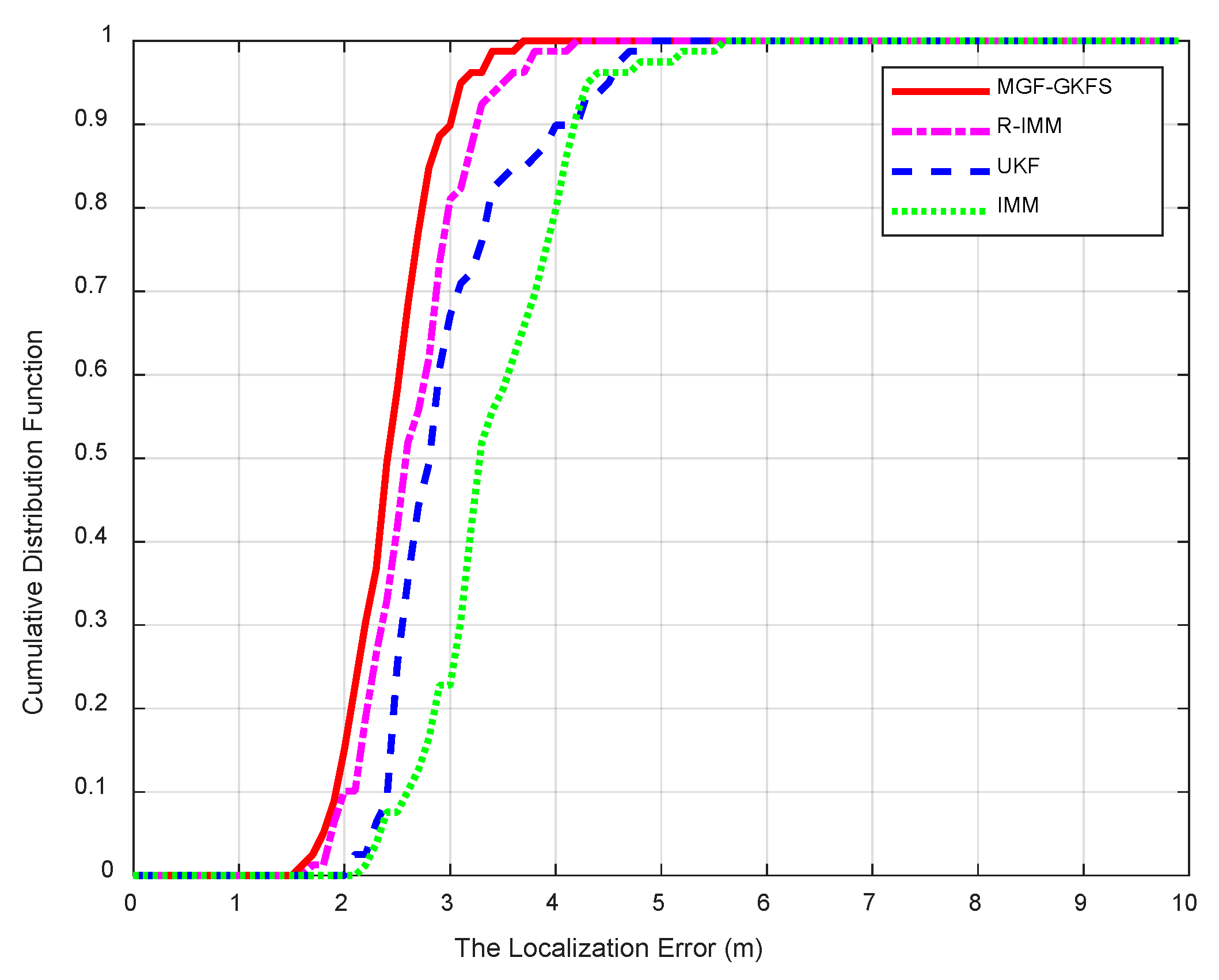
6.2. Experiment Results
6.3. Computational Analysis
7. Conclusions
Author Contributions
Funding
Conflicts of Interest
References
- Wang, Y.; Jie, H.H.; Cheng, L. A fusion localization method based on a robust extended kalman filter and track-quality for wireless sensor networks. Sensors 2019, 19, 3638. [Google Scholar] [CrossRef] [PubMed]
- Saeed, N.; Al-Naffouri, T.Y.; Alouini, M. Outlier detection and optimal anchor placement for 3-d underwater optical wireless sensor network localization. IEEE Trans. Commun. 2019, 67, 611–622. [Google Scholar] [CrossRef]
- Wang, T.; Xiong, H.; Ding, H.; Zheng, L. TDOA-based joint synchronization and localization algorithm for asynchronous wireless sensor networks. IEEE Trans. Commun. 2020, 68, 1981–1990. [Google Scholar] [CrossRef]
- Cheng, L.; Li, Y.F.; Wang, Y.; Bi, Y.Y.; Feng, L.; Xue, M.K. A triple-filter NLOS localization algorithm based on fuzzy c-means for wireless sensor networks. Sensors 2019, 19, 1215. [Google Scholar] [CrossRef]
- Hammes, U.; Zoubir, A.M. Robust Mobile Terminal Tracking in NLOS Environments Based on Data Association. IEEE Trans. Signal Process. 2010, 58, 5872–5882. [Google Scholar] [CrossRef]
- Tian, Q.; Wang, K.; Salcic, Z. A Low-Cost INS and UWB Fusion Pedestrian Tracking System. IEEE Sens. J. 2019, 19, 3733–3740. [Google Scholar] [CrossRef]
- Guvenc, I.; Chong, C.C. A survey on TOA based wireless localization and NLOS mitigation techniques. IEEE Commun. Surv. Tutor. 2009, 11, 107–124. [Google Scholar] [CrossRef]
- Cheng, L.; Wu, C.D.; Zhang, Y.Z. Indoor robot localization based on wireless sensor networks. IEEE Trans. Consum. Electron. 2011, 57, 1099–1104. [Google Scholar] [CrossRef]
- Cheng, L.; Hang, J.Q.; Wang, Y.; Bi, Y.Y. A fuzzy c-means and hierarchical voting based RSSI quantify localization method for wireless sensor network. IEEE Access 2019, 7, 47411–47422. [Google Scholar] [CrossRef]
- Amundson, I.; Sallai, J.; Koutsoukos, X.; Ledeczi, A. Mobile sensor waypoint navigation via RF-based angle of arrival localization. Int. J. Distrib. Sens. Netw. 2012, 8, 842107. [Google Scholar] [CrossRef]
- Cheng, L.; Wang, Y.; Wu, H.; Hu, N.; Wu, C.D. Non-parametric location estimation in rough wireless environments for wireless sensor network. Sens. Actuators A Phys. 2015, 224, 57–64. [Google Scholar] [CrossRef]
- Xu, K.; Liu, H.; Liu, D.; Huang, X.; Hou, F. Linear programming algorithms for sensor networks node localization. In Proceedings of the 2016 IEEE International Conference on Consumer Electronics (ICCE), Las Vegas, NV, USA, 7–11 January 2016; pp. 536–537. [Google Scholar]
- Xie, S.; Hu, Y.; Wang, Y. An improved E-Min-Max localization algorithm in wireless sensor networks. In Proceedings of the 2014 IEEE International Conference on Consumer Electronics, Shenzhen, China, 9–13 April 2014; pp. 1–4. [Google Scholar]
- Area-based, vs. multilateration localization: A comparative study of estimated position error. In Proceedings of the 2017 13th International Wireless Communications and Mobile Computing Conference (IWCMC), Valencia, Spain, 26–30 June 2017; pp. 1138–1143. [Google Scholar]
- Tomic, S.; Beko, M. A bisection-based approach for exact target localization in NLOS environments. Signal Process. 2018, 143, 328–335. [Google Scholar] [CrossRef]
- Tomic, S.; Beko, M.; Dinis, R.; Montezuma, P. A robust bisection-based estimator for TOA-based target localization in NLOS environments. IEEE Commun. Lett. 2017, 21, 2488–2491. [Google Scholar] [CrossRef]
- Tomic, S.; Beko, M. A robust NLOS bias mitigation technique for RSS-TOA-based target localization. IEEE Signal Process. Lett. 2019, 26, 64–68. [Google Scholar] [CrossRef]
- Yu, X.S.; Hu, N.; Xu, M.; Wu, M.C. A novel NLOS mobile node localization method in wireless sensor network. In Proceedings of the 4th International Conference on Communications, Signal Processing, and Systems, Chengdu, China, 23–24 October 2015; Volume 386, pp. 541–549. [Google Scholar]
- Yang, X.F. NLOS mitigation for UWB localization based on sparse pseudo-input gaussian process. IEEE Sens. J. 2018, 18, 4311–4316. [Google Scholar] [CrossRef]
- Guo, Q.; Ke, W.; Tang, W.C. Wireless positioning method based on dynamic objective function under mixed LOS/NLOS conditions. In Proceedings of the 2018 Ubiquitous Positioning, Indoor Navigation and Location-Based Services (UPINLBS), Wuhan, China, 22–23 March 2018; pp. 1–4. [Google Scholar]
- Han, K.; Xing, H.S.; Deng, Z.L.; Du, Y.C. A RSSI/PDR-based probabilistic position selection algorithm with NLOS identification for indoor localisation. ISPRS Int. J. Geo Inf. 2018, 7, 232. [Google Scholar] [CrossRef]
- Sun, J.L.; Wu, Z.L.; Yang, Z.D. SVM-CNN-based fusion algorithm for vehicle navigation considering atypical observations. IEEE Signal Process. Lett. 2019, 26, 212–216. [Google Scholar] [CrossRef]
- Miura, H.; Sakamoto, J.; Matsuda, N.; Taki, H.; Abe, N.; Hori, S. Adequate RSSI determination method by making use of SVM for indoor localization. In Proceedings of the 10th Knowledge-Based Intelligent Information and Engineering Systems, Bournemouth, UK, 9–11 October 2006; Volume 4252, pp. 628–636. [Google Scholar]
- Zou, H.; Huang, B.; Lu, X.; Jiang, H.; Xie, L. A robust indoor positioning system based on the procrustes analysis and weighted extreme learning machine. IEEE Trans. Wirel. Commun. 2016, 15, 1252–1266. [Google Scholar] [CrossRef]
- Yang, X.F.; Zhao, F.; Chen, T.J. NLOS identification for UWB localization based on import vector machine. AEU Int. J. Electron. Commun. 2018, 87, 128–133. [Google Scholar] [CrossRef]
- Julier, S.J.; Uhlmann, J.K. Unscented filtering and nonlinear estimation. Proc. IEEE 2004, 3, 401–422. [Google Scholar] [CrossRef]
- Feng, H.L.; Cai, Z.W. Target tracking based on improved square root cubature particle filter via underwater wireless sensor networks. IET Commun. 2019, 13, 1008–1015. [Google Scholar] [CrossRef]
- Chen, B.S.; Yang, C.Y.; Liao, J.F. Mobile location estimator in a rough wireless environment using extended kalman-based IMM and data fusion. IEEE Trans. Veh. Technol. 2004, 58, 1157–1169. [Google Scholar]
- Hammes, U.; Zoubir, A.M. Robust MT tracking based on M-estimation and interacting multiple model algorithm. IEEE Trans. Signal Process. 2011, 59, 3398–3409. [Google Scholar] [CrossRef]
- Hammes, U.; Wolsztynski, E.; Zoubir, A.M. Robust tracking and geolocation for wireless networks in NLOS Environments. IEEE J. Sel. Top. Signal Process. 2009, 3, 889–901. [Google Scholar] [CrossRef]
- Yuan, J.W.; Shi, Z.K. A method of vehicle tracking based on GM(1,1). Control Decis. 2006, 21, 300–304. [Google Scholar]
- Fu, Q.; Xiao, Y.S.; Yin, H.L. Object tracking algorithm based on grey innovation model GM(1,1) of fixed length. In Proceedings of the 2009 World Congress on Computer Science and Information Engineering, LOS Angeles, CA, USA, 31 March–2 April 2009; Volume 6, pp. 615–618. [Google Scholar]
- Huo, L.; Wang, Z.L. A target tracking algorithm using Grey Model predicting Kalman Filter in wireless sensor networks. In Proceedings of the 2017 IEEE International Conference on Internet of Things (iThings) and IEEE Green Computing and Communications (GreenCom) and IEEE Cyber, Physical and Social Computing (CPSCom) and IEEE Smart Data (SmartData), Exeter, UK, 21–23 June 2017; pp. 604–610. [Google Scholar]


| Symbol | Explanation | Symbol | Explanation |
|---|---|---|---|
| M | the number of beacon nodes | N | total time |
| the measured distance | the variance of sensor noise | ||
| the measured velocity | the initial state transition matrix | ||
| the updated state transition matrix in grey Kalman filter(GKF) | the state vector | ||
| the measurement vector | observation matrix | ||
| process noise | measurement noise | ||
| constant series length of predicting points | the filtered distance of GKF | ||
| the n-th element of original series of distance | original series of distance | ||
| the n-th element of accumulative series of distance | accumulative series of distance | ||
| development coefficient | grey effect coefficient | ||
| the n-th element of predicted series of distance | predicted series of distance | ||
| the n-th element of predicted accumulative series of distance | predicted accumulative series | ||
| accumulative series value of speed | the variance matrix of the state vector | ||
| the residual value between the measured distance and the filtered distance processed by GKF | the mean value of j-th single Gaussian distribution | ||
| the likelihood function of EM algorithm | G | the number of single Gaussian distribution | |
| the distribution parameter set of j-th single Gaussian distribution | the probability function that the residual value belongs to j-th Gaussian distribution at iteration t | ||
| the Euclidean distance between the current residual value and the small mean Gaussian distribution centre | the Euclidean distance between the current residual value and the big mean Gaussian distribution centre | ||
| the probability of LOS condition | the probability of NLOS condition | ||
| the final filtered distance | the filtered distance of UKF |
| Description | Notation | Default Values |
|---|---|---|
| The number of beacon nodes | M | 5 |
| The probability of line of sight (LOS )condition | 0.7 | |
| The sensor noise | 1 | |
| The total time of target moving | K | 80 |
| The number of Monte Carlo running | 1000 | |
| Gaussian distribution | ||
| Uniform distribution | ||
| Exponential distribution |
| Algorithm | Multiplications |
|---|---|
| MGF-GKFS | |
| R-IMM | |
| UKF | 59 |
| IMM | 98 |
| Algorithm | Running Time/s |
|---|---|
| MGF-GKFS | 0.0521 |
| R-IMM | 0.0221 |
| UKF | 0.0032 |
| IMM | 0.0128 |
© 2020 by the authors. Licensee MDPI, Basel, Switzerland. This article is an open access article distributed under the terms and conditions of the Creative Commons Attribution (CC BY) license (http://creativecommons.org/licenses/by/4.0/).
Share and Cite
Wang, Y.; Ren, W.; Cheng, L.; Zou, J. A Grey Model and Mixture Gaussian Residual Analysis-Based Position Estimator in an Indoor Environment. Sensors 2020, 20, 3941. https://doi.org/10.3390/s20143941
Wang Y, Ren W, Cheng L, Zou J. A Grey Model and Mixture Gaussian Residual Analysis-Based Position Estimator in an Indoor Environment. Sensors. 2020; 20(14):3941. https://doi.org/10.3390/s20143941
Chicago/Turabian StyleWang, Yan, Wenjia Ren, Long Cheng, and Jijun Zou. 2020. "A Grey Model and Mixture Gaussian Residual Analysis-Based Position Estimator in an Indoor Environment" Sensors 20, no. 14: 3941. https://doi.org/10.3390/s20143941
APA StyleWang, Y., Ren, W., Cheng, L., & Zou, J. (2020). A Grey Model and Mixture Gaussian Residual Analysis-Based Position Estimator in an Indoor Environment. Sensors, 20(14), 3941. https://doi.org/10.3390/s20143941