Encoding Time Series as Multi-Scale Signed Recurrence Plots for Classification Using Fully Convolutional Networks


Abstract
1. Introduction
2. Approaches
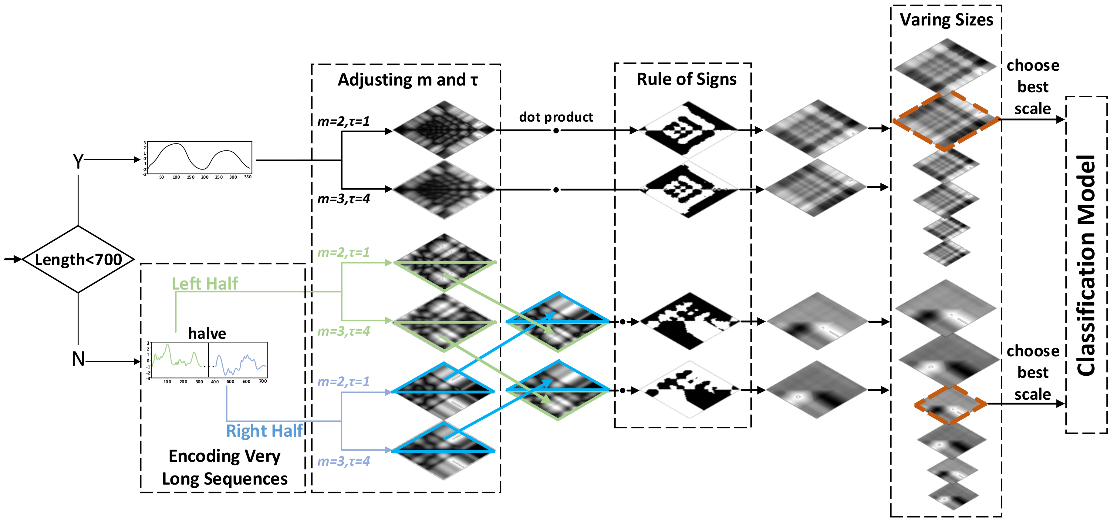
2.1. Proposed MS-RP
2.1.1. Review of RP
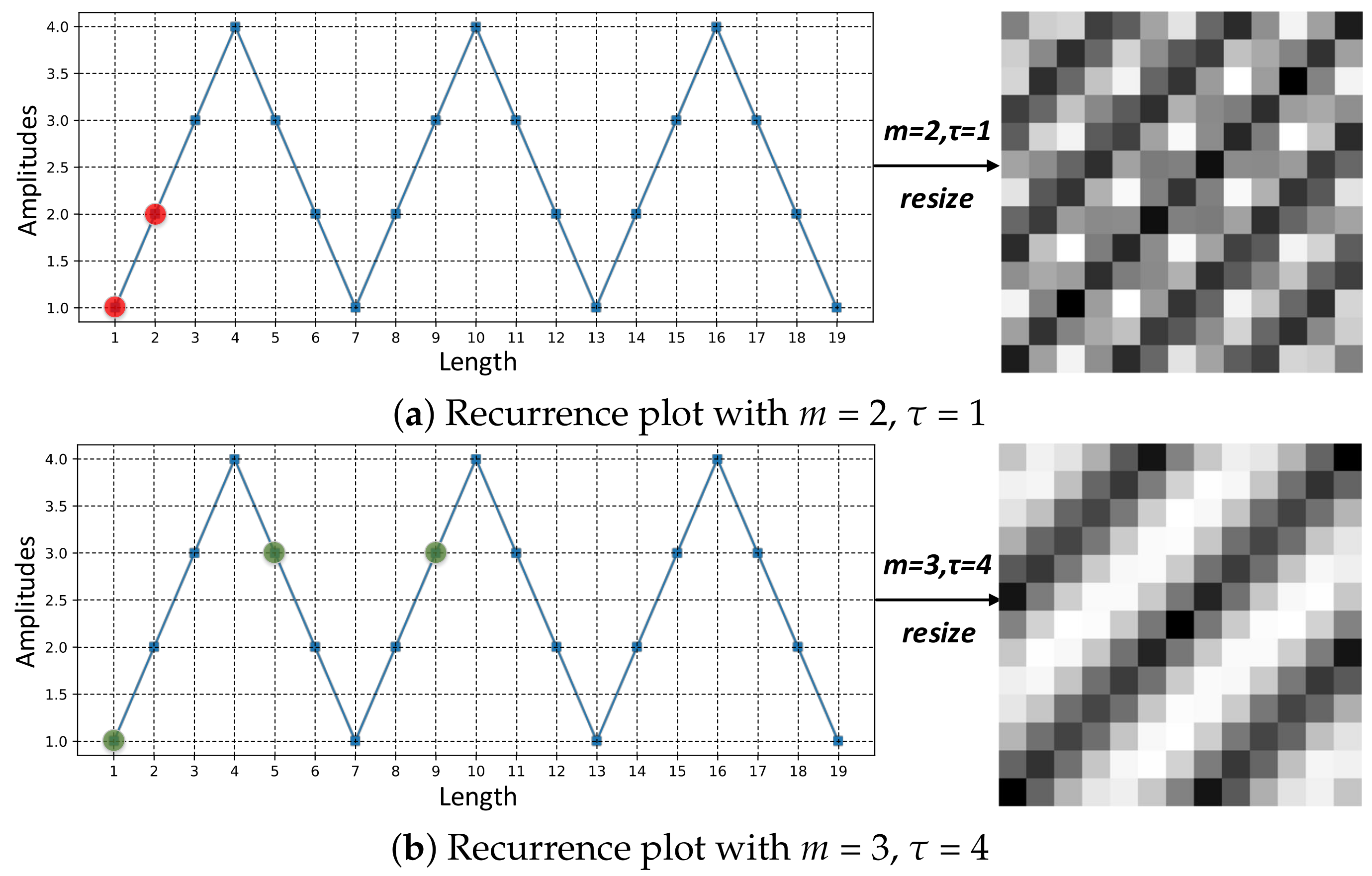
2.1.2. Multi-Scale RP: An Improvement of RP
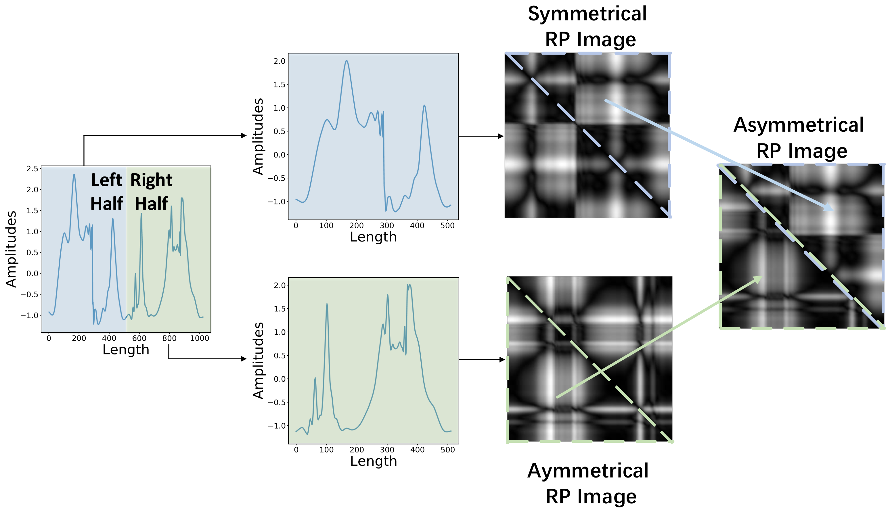
2.1.3. Asymmetrical RP for Encoding Very Long Sequences
2.1.4. Rule of Signs
2.2. Classification Using FCN on MS-RP Images
3. Experiments and Analysis
3.1. Experimental Setup
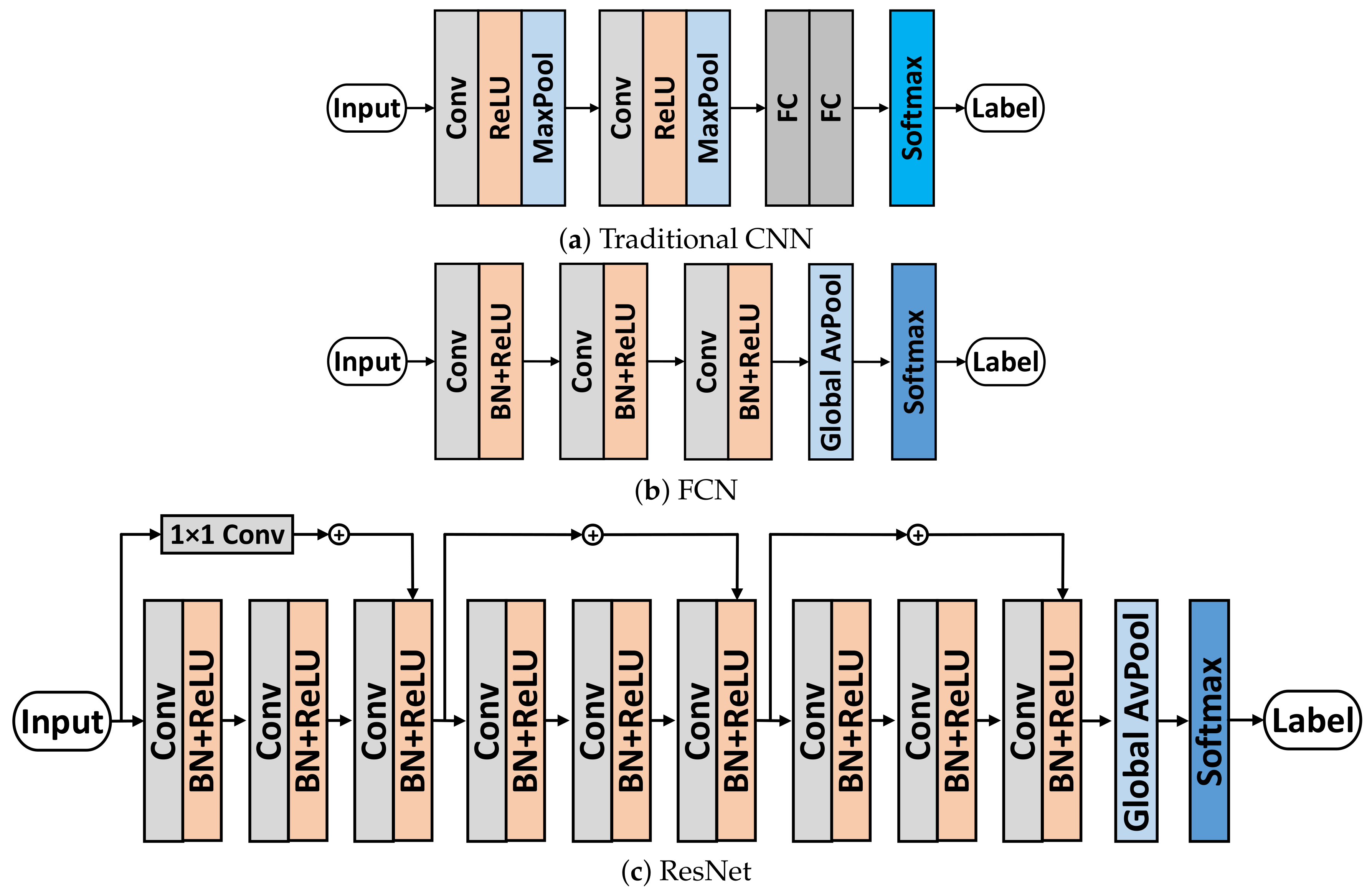
- FCN and ResNet: These two models are proposed in [19], which have been regarded as the strong baseline and best DNN-based classifiers for TSC.
- RP-CNN: [26] combines RP with a traditional CNN, which is similar to our proposed approach. We take it as the baseline for methods encoding time series as images. The RP image sizes are consistent with our approach for fairness, and (m, ) of RP are (3, 4). The architecture of traditional CNN is shown in Figure 7a. The traditional CNN consists of two convolutional layers (32 channels, 3 × 3 kernel), two pooling layers (2 × 2 Max Pooling), two FC layers (125 neurons), and a Softmax layer.
- RP-FCN: This model combines RP and FCN into one frame work. It is provided by us for comparison between RP and MS-RP.
- HIVE-COTE: This model ensembles five different features with various heterogeneous classifiers [17]; it achieves state-of-the-art performance among traditional time series classification methods.
- FCN Residual Classification Flow (FCN-RCF): [20] decomposes sequences as multiple frequencies of subsequences through fine-grained wavelet, and FCN are then applied to handle these subsequences. This model achieves very strong performances.
- ALSTM-FCN: This model combines FCN and ALSTM in one framework [21]. ALSTM supplements important temporal information for FCN, which obviously improves classification performance. The proposed ALSTM-FCN achieves state-of-the-art performance among DNN based methods.
3.2. Results and Analysis
3.3. Visualization
4. Conclusions
Author Contributions
Funding
Conflicts of Interest
References
- Ying, T.; Shi, Y. Data Mining and Big Data. IEEE Trans. Knowl. Data Eng. 2016, 26, 97–107. [Google Scholar]
- Bagnall, A.; Lines, J.; Bostrom, A.; Large, J.; Keogh, E. The great time series classification bake off: A review and experimental evaluation of recent algorithmic advances. Data Min. Knowl. Discov. 2017, 31, 606–660. [Google Scholar] [CrossRef] [PubMed]
- Fawaz, H.I.; Forestier, G.; Weber, J.; Idoumghar, L.; Muller, P.A. Deep learning for time series classification: A review. Data Min. Knowl. Discov. 2019, 33, 917–963. [Google Scholar] [CrossRef]
- Senin, P.; Malinchik, S. Sax-vsm: Interpretable time series classification using sax and vector space model. In Proceedings of the 2013 IEEE 13th International Conference on Data Mining, Dallas, TX, USA, 7–10 December 2013; IEEE: Piscataway, NJ, USA, 2013; pp. 1175–1180. [Google Scholar]
- Hills, J.; Lines, J.; Baranauskas, E.; Mapp, J.; Bagnall, A. Classification of time series by shapelet transformation. Data Min. Knowl. Discov. 2014, 28, 851–881. [Google Scholar] [CrossRef]
- Grabocka, J.; Schilling, N.; Wistuba, M.; Schmidt-Thieme, L. Learning time-series shapelets. In Proceedings of the 20th ACM SIGKDD International Conference on Knowledge Discovery and Data Mining, New York, NY, USA, 24–27 August 2014; pp. 392–401. [Google Scholar]
- Schäfer, P. The BOSS is concerned with time series classification in the presence of noise. Data Min. Knowl. Discov. 2015, 29, 1505–1530. [Google Scholar] [CrossRef]
- Zhu, H.; Hu, J.; Chang, S.; Lu, L. ShakeIn: Secure user authentication of smartphones with single-handed shakes. IEEE Trans. Mob. Comput. 2017, 16, 2901–2912. [Google Scholar] [CrossRef]
- Yao, L.; Li, Y.; Li, Y.; Zhang, H.; Huai, M.; Gao, J.; Zhang, A. DTEC: Distance Transformation Based Early Time Series Classification. In Proceedings of the 2019 SIAM International Conference on Data Mining, Calgary, AB, Canada, 2–4 May 2019; pp. 486–494. [Google Scholar]
- Roychoudhury, S.; Zhou, F.; Obradovic, Z. Leveraging Subsequence-orders for Univariate and Multivariate Time-series Classification. In Proceedings of the 2019 SIAM International Conference on Data Mining, Calgary, AB, Canada, 2–4 May 2019; pp. 495–503. [Google Scholar]
- Sakoe, H.; Chiba, S. Dynamic programming algorithm optimization for spoken word recognition. IEEE Trans. Acoust. Speech Signal Process. 1978, 26, 43–49. [Google Scholar] [CrossRef]
- Jeong, Y.S.; Jeong, M.K.; Omitaomu, O.A. Weighted dynamic time warping for time series classification. Pattern Recognit. 2011, 44, 2231–2240. [Google Scholar] [CrossRef]
- Lines, J.; Bagnall, A. Time series classification with ensembles of elastic distance measures. Data Min. Knowl. Discov. 2015, 29, 565–592. [Google Scholar] [CrossRef]
- Tan, C.W.; Herrmann, M.; Forestier, G.; Webb, G.I.; Petitjean, F. Efficient search of the best warping window for dynamic time warping. In Proceedings of the 2018 SIAM International Conference on Data Mining, San Diego, CA, USA, 3–5 May 2018; pp. 225–233. [Google Scholar]
- Tan, C.W.; Petitjean, F.; Webb, G.I. Elastic bands across the path: A new framework and method to lower bound DTW. In Proceedings of the 2019 SIAM International Conference on Data Mining, Calgary, AB, Canada, 2–4 May 2019; pp. 522–530. [Google Scholar]
- Bagnall, A.; Lines, J.; Hills, J.; Bostrom, A. Time-series classification with COTE: The collective of transformation-based ensembles. IEEE Trans. Knowl. Data Eng. 2015, 27, 2522–2535. [Google Scholar] [CrossRef]
- Lines, J.; Taylor, S.; Bagnall, A. Time series classification with HIVE-COTE: The hierarchical vote collective of transformation-based ensembles. ACM Trans. Knowl. Discov. Data (TKDD) 2018, 12, 52. [Google Scholar] [CrossRef]
- Cui, Z.; Chen, W.; Chen, Y. Multi-scale convolutional neural networks for time series classification. arXiv 2016, arXiv:1603.06995. [Google Scholar]
- Wang, Z.; Yan, W.; Oates, T. Time series classification from scratch with deep neural networks: A strong baseline. In Proceedings of the 2017 international joint conference on neural networks (IJCNN), Anchorage, AK, USA, 14–19 May 2017; IEEE: Piscataway, NJ, USA, 2017; pp. 1578–1585. [Google Scholar]
- Wang, J.; Wang, Z.; Li, J.; Wu, J. Multilevel wavelet decomposition network for interpretable time series analysis. In Proceedings of the 24th ACM SIGKDD International Conference on Knowledge Discovery & Data Mining, London, UK, 19–23 August 2018; pp. 2437–2446. [Google Scholar]
- Karim, F.; Majumdar, S.; Darabi, H.; Chen, S. LSTM fully convolutional networks for time series classification. IEEE Access 2017, 6, 1662–1669. [Google Scholar] [CrossRef]
- Wang, Z.; Oates, T. Encoding time series as images for visual inspection and classification using tiled convolutional neural networks. In Proceedings of the Workshops at the Twenty-Ninth AAAI Conference on Artificial Intelligence, Austin, TX, USA, 25–30 January 2015. [Google Scholar]
- Wang, Z.; Oates, T. Imaging time-series to improve classification and imputation. In Proceedings of the Twenty-Fourth International Joint Conference on Artificial Intelligence, Buenos Aires, Argentina, 25–31 July 2015. [Google Scholar]
- Yang, C.L.; Chen, Z.X.; Yang, C.Y. Sensor Classification Using Convolutional Neural Network by Encoding Multivariate Time Series as Two-Dimensional Colored Images. Sensors 2020, 20, 168. [Google Scholar] [CrossRef] [PubMed]
- Qin, Z.; Zhang, Y.; Meng, S.; Qin, Z.; Choo, K.K.R. Imaging and fusing time series for wearable sensor-based human activity recognition. Inf. Fusion 2020, 53, 80–87. [Google Scholar] [CrossRef]
- Hatami, N.; Gavet, Y.; Debayle, J. Classification of time-series images using deep convolutional neural networks. Int. Soc. Opt. Photonics 2018, 10696, 106960Y. [Google Scholar]
- Long, J.; Shelhamer, E.; Darrell, T. Fully convolutional networks for semantic segmentation. In Proceedings of the IEEE Conference on Computer Vision and Pattern Recognition, Boston, MA, USA, 7–12 June 2015; pp. 3431–3440. [Google Scholar]
- He, K.; Zhang, X.; Ren, S.; Sun, J. Deep residual learning for image recognition. In Proceedings of the IEEE conference on computer vision and pattern recognition, Las Vegas, NV, USA, 27–30 June 2016; pp. 770–778. [Google Scholar]
- Szegedy, C.; Ioffe, S.; Vanhoucke, V.; Alemi, A.A. Inception-v4, inception-resnet and the impact of residual connections on learning. In Proceedings of the Thirty-First, AAAI Conference on Artificial Intelligence, San Francisco, CA, USA, 4–9 February 2017. [Google Scholar]
- Eckmann, J.P.; Kamphorst, S.O.; Ruelle, D. Recurrence Plots of Dynamical Systems. Eur. Lett. 1987, 4, 973–977. [Google Scholar] [CrossRef]
- Marwan, N.; Romano, M.C.; Thiel, M.; Kurths, J. Recurrence plots for the analysis of complex systems. Phys. Rep. 2007, 438, 237–329. [Google Scholar] [CrossRef]
- Silva, D.F.; De Souza, V.M.; Batista, G.E. Time series classification using compression distance of recurrence plots. In Proceedings of the 2013 IEEE 13th International Conference on Data Mining, Dallas, TX, USA, 7–10 December 2013; pp. 687–696. [Google Scholar]
- Hatami, N.; Gavet, Y.; Debayle, J. Bag of recurrence patterns representation for time-series classification. Pattern Anal. Appl. 2019, 22, 877–887. [Google Scholar] [CrossRef]
- Souza, V.M.; Silva, D.F.; Batista, G.E. Extracting texture features for time series classification. In Proceedings of the 2014 22nd International Conference on Pattern Recognition, Stockholm, Sweden, 24–28 August 2014; IEEE: Piscataway, NJ, USA, 2014; pp. 1425–1430. [Google Scholar]
- Dau, H.A.; Bagnall, A.; Kamgar, K.; Yeh, C.C.M.; Zhu, Y.; Gharghabi, S.; Ratanamahatana, C.A.; Keogh, E. The UCR time series archive. arXiv 2018, arXiv:1810.07758. [Google Scholar] [CrossRef]
- Maaten, L.v.d.; Hinton, G. Visualizing data using t-SNE. J. Mach. Learn. Res. 2008, 9, 2579–2605. [Google Scholar]
- Garcia-Ceja, E.; Uddin, M.Z.; Torresen, J. Classification of recurrence plots’ distance matrices with a convolutional neural network for activity recognition. Procedia Comput. Sci. 2018, 130, 157–163. [Google Scholar] [CrossRef]
- Kingma, D.P.; Ba, J. Adam: A method for stochastic optimization. arXiv 2014, arXiv:1412.6980. [Google Scholar]
- Demšar, J. Statistical comparisons of classifiers over multiple data sets. J. Mach. Learn. Res. 2006, 7, 1–30. [Google Scholar]
- Friedman, M. A comparison of alternative tests of significance for the problem of m rankings. Ann. Math. Stat. 1940, 11, 86–92. [Google Scholar] [CrossRef]
- Garcia, S.; Herrera, F. An extension on “statistical comparisons of classifiers over multiple data sets” for all pairwise comparisons. J. Mach. Learn. Res. 2008, 9, 2677–2694. [Google Scholar]
- Benavoli, A.; Corani, G.; Mangili, F. Should we really use post-hoc tests based on mean-ranks? J. Mach. Learn. Res. 2016, 17, 152–161. [Google Scholar]


| Network Parameters | Convolution Blocks | ||
|---|---|---|---|
| Conv1 | Conv2 | Conv3 | |
| Conv Kernel Size | 5 × 5 | 5 × 5 | 5 × 5 |
| Filter Channel Number | 128 | 256 | 128 |
| Dataset | RP-CNN | Res-Net | FCN | RP-FCN | HIVE-COTE | FCN-RCF | ALSTM-FCN | MS-RP-Res | MS-RP-FCN |
|---|---|---|---|---|---|---|---|---|---|
| Adiac(64,2,1) | 0.2800 | 0.1740 | 0.1430 | 0.1709 | 0.1846 | 0.1550 | 0.1330 | 0.1560 | 0.1379 |
| Beef(64,2,1) | 0.0800 | 0.2330 | 0.2500 | 0.1667 | 0.2773 | 0.0300 | 0.0667 | 0.0667 | 0.1333 |
| CBF(64,2,1) | 0.0050 | 0.0060 | 0 | 0.0033 | 0.0006 | 0 | 0 | 0 | 0 |
| ChlorineCon(112,2,1) | 0.1049 | 0.1720 | 0.1570 | 0.1992 | 0.2749 | 0.0680 | 0.1930 | 0.1987 | 0.1992 |
| CinTorso(128,3,4) | 0.0087 | 0.2290 | 0.1870 | 0.2866 | 0.0120 | 0.0140 | 0.0942 | 0.0486 | 0.1123 |
| Coffee(64,2,1) | 0 | 0 | 0 | 0 | 0.0018 | 0 | 0 | 0 | 0 |
| CricketX(64,3,4) | 0.2718 | 0.1790 | 0.1850 | 0.2187 | 0.1696 | 0.2160 | 0.1949 | 0.1538 | 0.1821 |
| CricketY(64,3,4) | 0.2462 | 0.1950 | 0.2080 | 0.2349 | 0.1630 | 0.1720 | 0.1795 | 0.1564 | 0.1718 |
| CricketZ(64,3,4) | 0.2667 | 0.1870 | 0.1870 | 0.2064 | 0.1523 | 0.1620 | 0.1692 | 0.1487 | 0.1615 |
| DiatomSizeR(64,2,1) | 0.0098 | 0.0690 | 0.0700 | 0.0196 | 0.0581 | 0.0230 | 0.0261 | 0.0065 | 0.0098 |
| ECG200(64,2,1) | 0 | 0.1300 | 0.1000 | 0.0800 | 0.1181 | 0.0625 | 0.0900 | 0.0500 | 0.0800 |
| ECGFiveDays(64,3,4) | 0.0023 | 0.0450 | 0.0150 | 0 | 0.0105 | 0.0100 | 0.0046 | 0 | 0 |
| FaceAll(96,2,1) | 0.1900 | 0.1660 | 0.0710 | 0.1775 | 0.0037 | 0.0980 | 0.0343 | 0.0627 | 0.0320 |
| FaceFour(96,2,1) | 0 | 0.0680 | 0.0680 | 0.0341 | 0.0505 | 0.0500 | 0.0568 | 0.0795 | 0.0400 |
| FacesUCR(64,2,1) | 0.0483 | 0.0420 | 0.0520 | 0.0751 | 0.0164 | 0.0870 | 0.0566 | 0.0585 | 0.0561 |
| FiftyWords(48,3,4) | 0.2600 | 0.2730 | 0.3210 | 0.1846 | 0.1932 | 0.2880 | 0.1758 | 0.1692 | 0.1780 |
| Fish(64,2,1) | 0.0850 | 0.0110 | 0.0290 | 0 | 0.0238 | 0.0210 | 0.0229 | 0.0114 | 0 |
| GunPoint(64,2,1) | 0 | 0.0070 | 0 | 0 | 0.0033 | 0 | 0 | 0 | 0 |
| Haptics(64,2,1) | 0.5390 | 0.4940 | 0.4490 | 0.4578 | 0.4697 | 0.4610 | 0.4351 | 0.4708 | 0.4675 |
| InlineSkate(128,2,1) | 0.6436 | 0.6350 | 0.5890 | 0.5382 | 0.4741 | 0.5660 | 0.5073 | 0.5655 | 0.5491 |
| ItaPowDemand(16,2,1) | 0.0330 | 0.0400 | 0.0300 | 0.0447 | 0.0322 | 0.0310 | 0.0398 | 0.0262 | 0.0292 |
| Lightning2(64,3,4) | 0.1639 | 0.2460 | 0.1970 | 0.0984 | 0.2030 | 0.1450 | 0.2131 | 0.1148 | 0.0984 |
| Lightning7(64,3,4) | 0.2600 | 0.1640 | 0.1370 | 0.1470 | 0.1889 | 0.0910 | 0.1781 | 0.1440 | 0.1233 |
| Mallat(128,3,4) | 0.0512 | 0.0210 | 0.0200 | 0.0752 | 0.0245 | 0.0440 | 0.0162 | 0.0473 | 0.0422 |
| MedicalImg(96,2,1) | 0.2658 | 0.2280 | 0.2080 | 0.2329 | 0.1846 | 0.1640 | 0.2039 | 0.2066 | 0.1947 |
| MoteStrain(80,2,1) | 0.1182 | 0.1050 | 0.0500 | 0.1741 | 0.0532 | 0.0760 | 0.0639 | 0.0847 | 0.0831 |
| NonInThorax1(128,3,4) | 0.0580 | 0.0520 | 0.0390 | 0.0580 | 0.0683 | 0.0260 | 0.0249 | 0.0575 | 0.0361 |
| NonInThorax2(128,3,4) | 0.0489 | 0.0490 | 0.0450 | 0.0579 | 0.0477 | 0.0280 | 0.0336 | 0.0453 | 0.0366 |
| OliveOil(96,2,1) | 0.1100 | 0.1330 | 0.1670 | 0.1333 | 0.1023 | 0 | 0.0667 | 0.0667 | 0.0500 |
| OSULeaf(96,2,1) | 0.2900 | 0.0210 | 0.0120 | 0.0909 | 0.0295 | 0.0180 | 0.0041 | 0.0248 | 0.0165 |
| SonyAIRobot1(64,2,1) | 0.0499 | 0.0150 | 0.0320 | 0.0266 | 0.1132 | 0.0420 | 0.0300 | 0.0166 | 0.0067 |
| SonyAIRobot2(64,2,1) | 0.0923 | 0.0380 | 0.0380 | 0.0546 | 0.0546 | 0.0640 | 0.0252 | 0.0535 | 0.0210 |
| StarLigCurves(128,3,4) | 0.0234 | 0.0250 | 0.0330 | 0.0238 | 0.0185 | 0.0180 | 0.0233 | 0.0195 | 0.0180 |
| SwedishLeaf(64,2,1) | 0.0600 | 0.0420 | 0.0340 | 0.0304 | 0.0314 | 0.0570 | 0.0144 | 0.0272 | 0.0272 |
| Symbols(64,3,4) | 0.0824 | 0.1280 | 0.0380 | 0.0181 | 0.0342 | 0.0400 | 0.0131 | 0.0141 | 0.0161 |
| SynControl(64,2,1) | 0.3433 | 0 | 0.0100 | 0.3100 | 0.0004 | 0.0382 | 0.0100 | 0 | 0 |
| Trace(64,2,1) | 0 | 0 | 0 | 0 | 0 | 0.0940 | 0 | 0 | 0 |
| TwoLeadECG(64,2,1) | 0.0026 | 0 | 0 | 0.0018 | 0.0065 | 0.0643 | 0.0009 | 0 | 0 |
| TwoPatterns(64,2,1) | 0.4935 | 0 | 0.1030 | 0.4888 | 0.0001 | 0 | 0.0032 | 0 | 0 |
| UWaveX(64,3,4) | 0.3582 | 0.2130 | 0.2460 | 0.3778 | 0.1616 | 0.2180 | 0.1519 | 0.1790 | 0.1963 |
| UWaveY(64,3,4) | 0.3439 | 0.3320 | 0.2750 | 0.3425 | 0.2245 | 0.2320 | 0.2342 | 0.2496 | 0.2725 |
| UWaveZ(64,2,1) | 0.3317 | 0.2450 | 0.2710 | 0.3490 | 0.2217 | 0.2650 | 0.2018 | 0.2272 | 0.2462 |
| Wafer(64,2,1) | 0 | 0.0030 | 0.0030 | 0.0015 | 0.0003 | 0 | 0.0019 | 0.0006 | 0.0011 |
| WoSynonyms(64,2,1) | 0.3135 | 0.3680 | 0.4200 | 0.2900 | 0.2520 | 0.3380 | 0.3323 | 0.2774 | 0.2978 |
| Yoga(64,2,1) | 0.1180 | 0.1420 | 0.1550 | 0.0953 | 0.0830 | 0.1120 | 0.0810 | 0.0887 | 0.0930 |
| Win num | 7 | 5 | 6 | 6 | 6 | 11 | 14 | 14 | 13 |
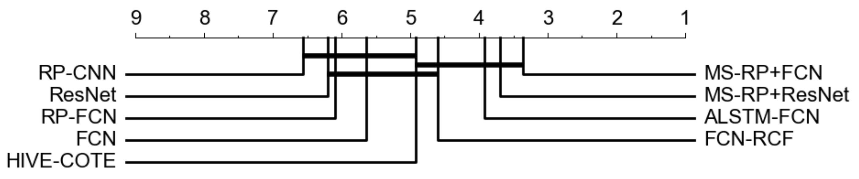
| Arithmetic ranking | 6.3111 | 5.9111 | 5.2889 | 5.7778 | 4.8444 | 4.3778 | 3.6444 | 3.3111 | 2.9111 |
| Geometric ranking | 5.0800 | 4.9744 | 4.3512 | 4.7974 | 3.8710 | 3.4003 | 2.8214 | 2.6007 | 2.4147 |
| MPCE | 0.0256 | 0.0240 | 0.0220 | 0.0252 | 0.0203 | 0.0175 | 0.0175 | 0.0164 | 0.0164 |
| Dataset | Adiac | Face- All | Medical- Img | Mote- Strain | OSU- Leaf | CricketY | CricketZ | Fifty- Words | Lightning2 | Lightning7 |
|---|---|---|---|---|---|---|---|---|---|---|
| m = 2, = 1 | 0.1379 | 0.0320 | 0.1947 | 0.0831 | 0.0165 | 0.2077 | 0.1897 | 0.2066 | 0.1475 | 0.1507 |
| m = 3, = 4 | 0.1637 | 0.0698 | 0.2316 | 0.1222 | 0.0620 | 0.1718 | 0.1615 | 0.1780 | 0.0984 | 0.1233 |
| Dataset | CinTorso | InlineSkate | Mallat | NonInThorax1 | NonInThorax2 | StarLigCurves |
|---|---|---|---|---|---|---|
| Asymmetric RP | 0.1123 | 0.5491 | 0.0422 | 0.0361 | 0.0366 | 0.0180 |
| Symmetric RP | 0.2866 | 0.5382 | 0.0729 | 0.0539 | 0.0514 | 0.0232 |
| Dataset | CricketX | CricketY | CricketZ | Lightning7 | OSU- Leaf | Syn- Control | Two- Patterns | UWaveX | UWaveY | UWaveZ |
|---|---|---|---|---|---|---|---|---|---|---|
| Signed RP | 0.1821 | 0.1718 | 0.1615 | 0.1233 | 0.0165 | 0 | 0 | 0.1963 | 0.2725 | 0.2462 |
| Unsigned RP | 0.2187 | 0.2349 | 0.2064 | 0.1469 | 0.0744 | 0.2967 | 0.4850 | 0.3778 | 0.3425 | 0.3431 |
© 2020 by the authors. Licensee MDPI, Basel, Switzerland. This article is an open access article distributed under the terms and conditions of the Creative Commons Attribution (CC BY) license (http://creativecommons.org/licenses/by/4.0/).
Share and Cite
Zhang, Y.; Hou, Y.; Zhou, S.; Ouyang, K. Encoding Time Series as Multi-Scale Signed Recurrence Plots for Classification Using Fully Convolutional Networks. Sensors 2020, 20, 3818. https://doi.org/10.3390/s20143818
Zhang Y, Hou Y, Zhou S, Ouyang K. Encoding Time Series as Multi-Scale Signed Recurrence Plots for Classification Using Fully Convolutional Networks. Sensors. 2020; 20(14):3818. https://doi.org/10.3390/s20143818
Chicago/Turabian StyleZhang, Ye, Yi Hou, Shilin Zhou, and Kewei Ouyang. 2020. "Encoding Time Series as Multi-Scale Signed Recurrence Plots for Classification Using Fully Convolutional Networks" Sensors 20, no. 14: 3818. https://doi.org/10.3390/s20143818
APA StyleZhang, Y., Hou, Y., Zhou, S., & Ouyang, K. (2020). Encoding Time Series as Multi-Scale Signed Recurrence Plots for Classification Using Fully Convolutional Networks. Sensors, 20(14), 3818. https://doi.org/10.3390/s20143818