Separable EEG Features Induced by Timing Prediction for Active Brain-Computer Interfaces

 , ,
, ,
Abstract
1. Introduction
2. Materials and Methods
2.1. Participants
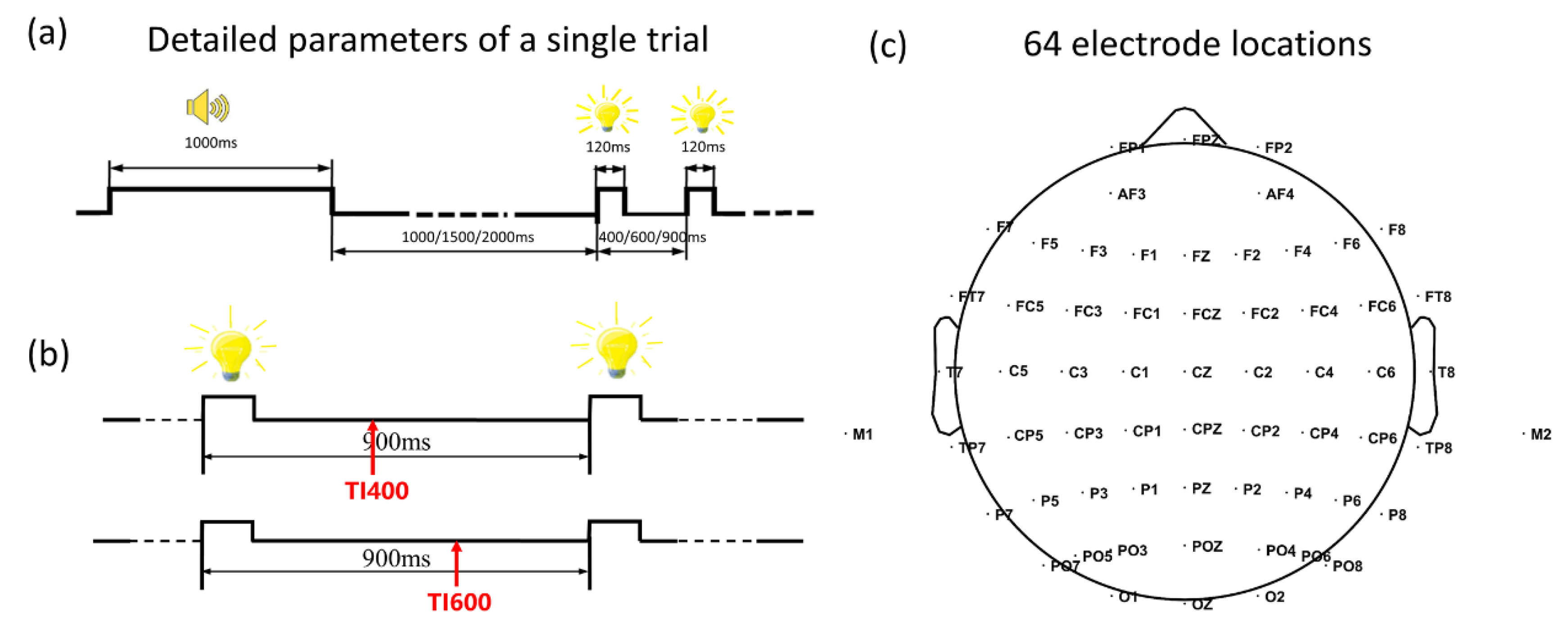
2.2. Stimuli
2.3. Experimental Procedure
2.4. EEG Recording and Pre-Processing
2.5. Feature Extraction and Pattern Classification
2.5.1. Discriminative Canonical Pattern Matching (DCPM)
2.5.2. Common Spatial Patterns (CSP)
2.5.3. The Decision-Fusion of DCPM and CSP
3. Results
3.1. Behavioral Performances
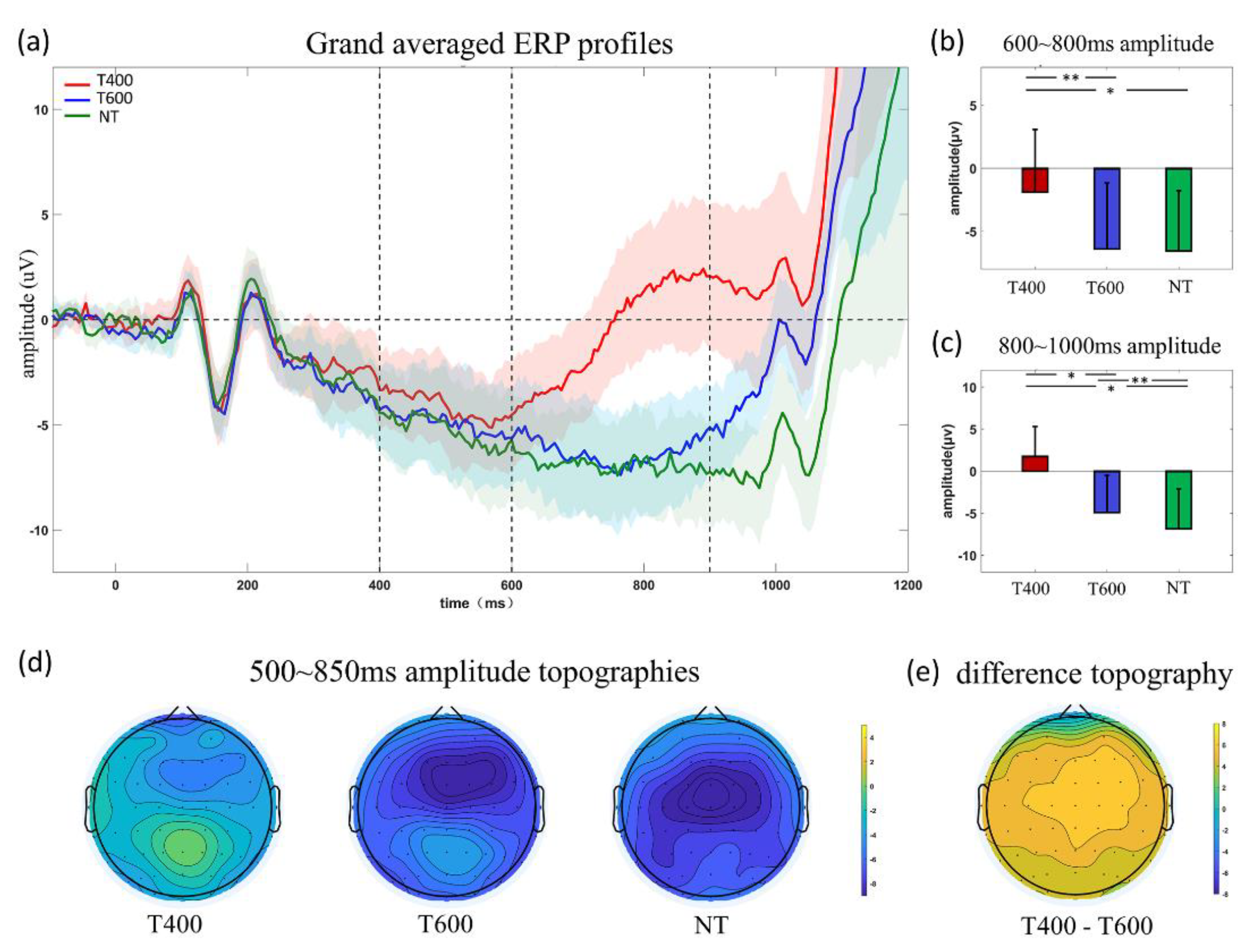
3.2. ERP Analyses
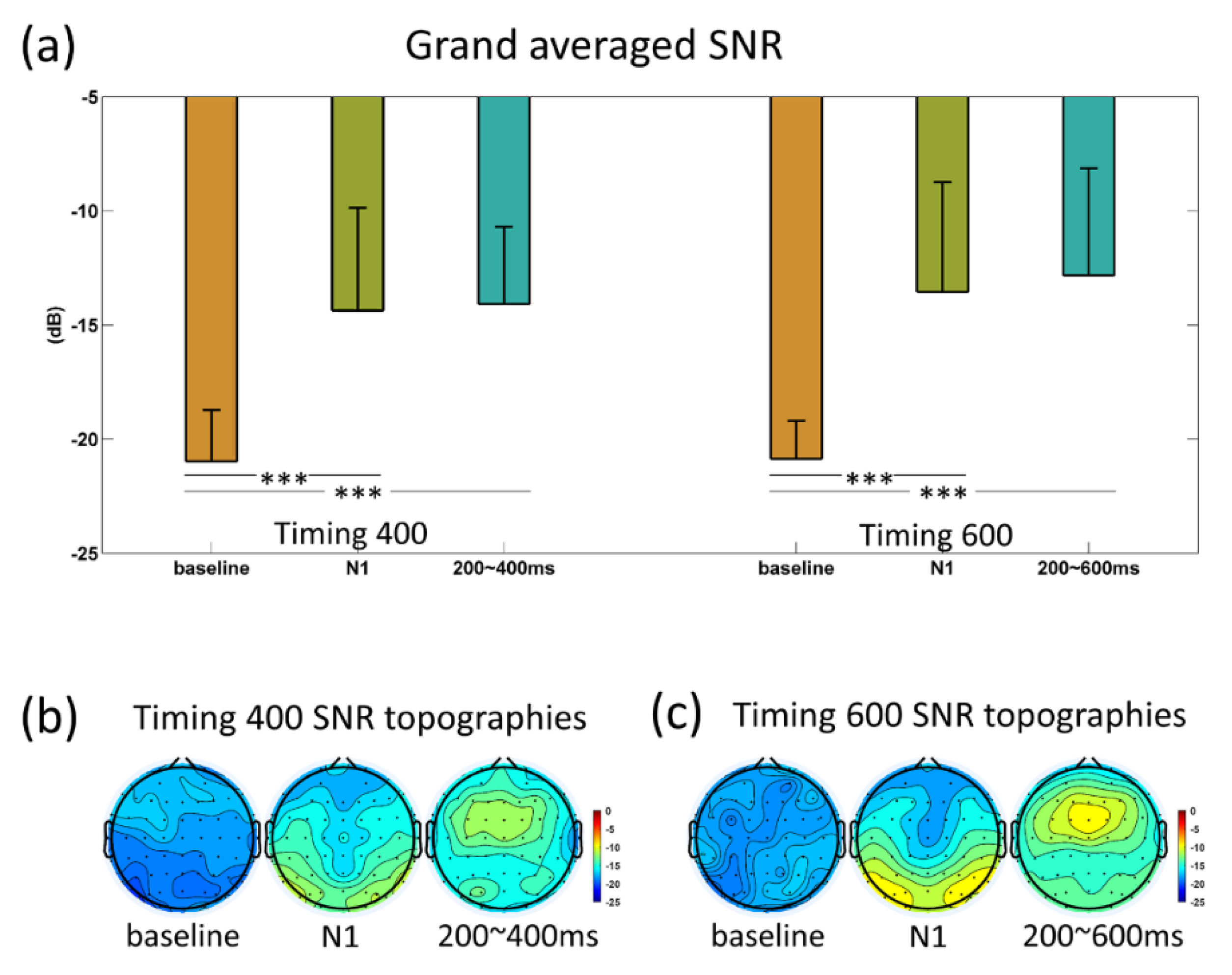
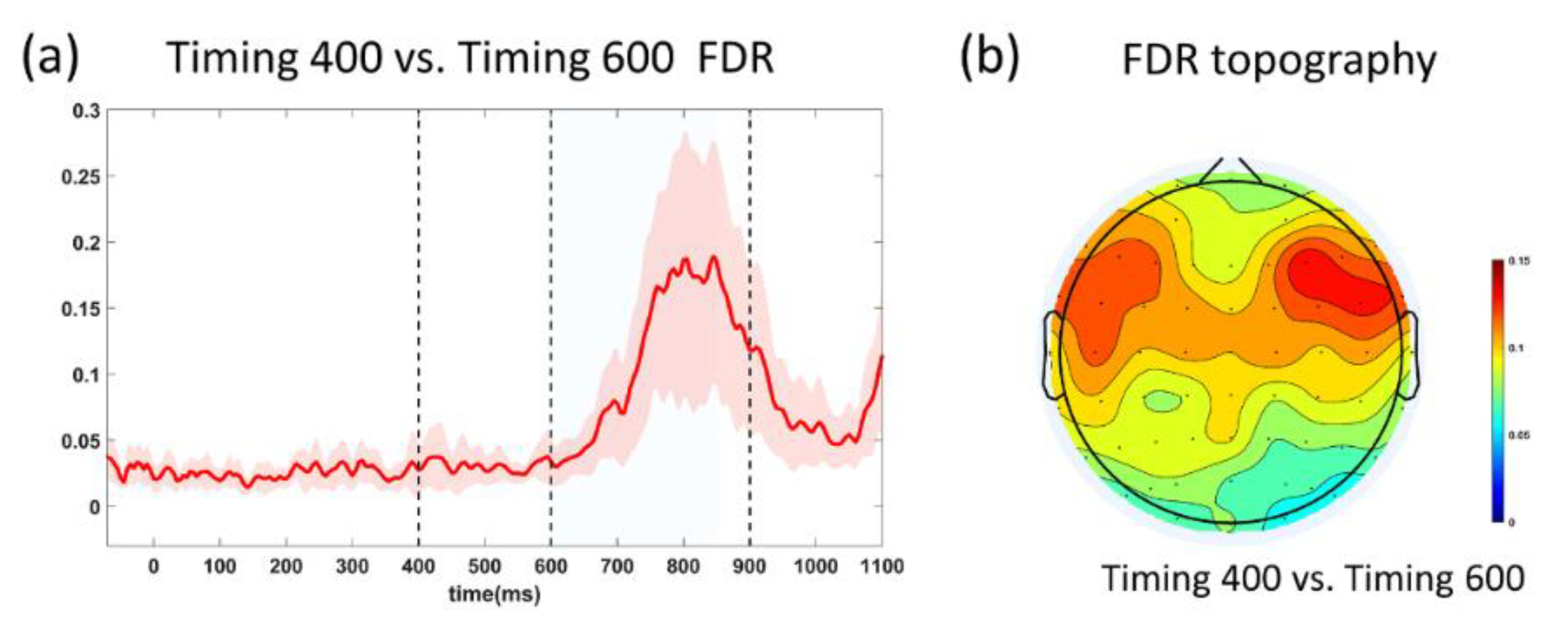
3.3. SNR and FDR Analyses
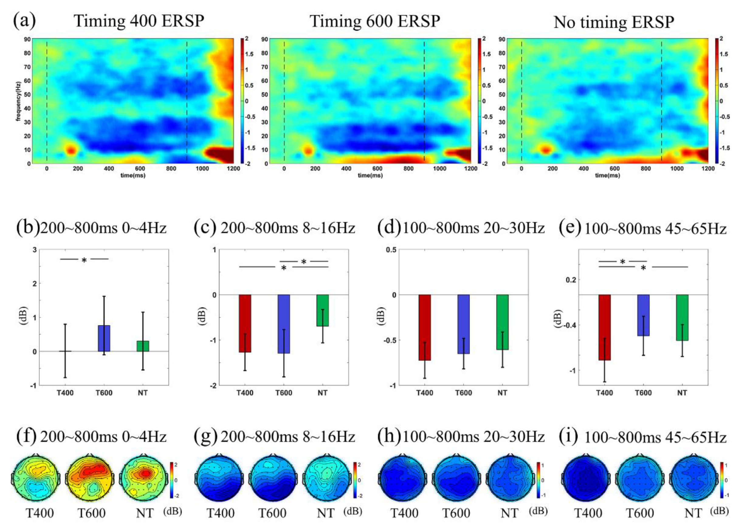
3.4. ERSP Analyses
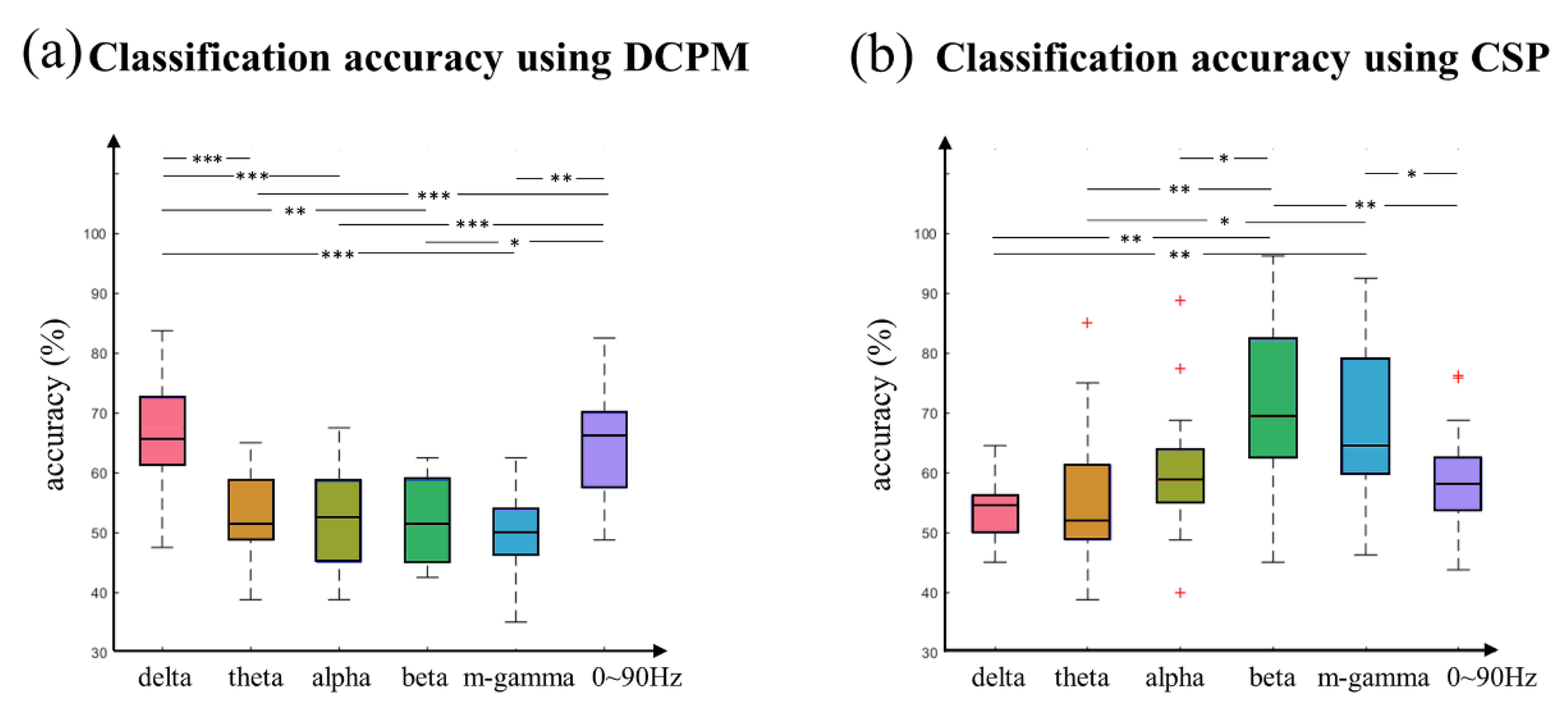
3.5. Classification Performance
4. Discussion
5. Conclusions
Supplementary Materials
Author Contributions
Funding
Acknowledgments
Conflicts of Interest
References
- Lebedev, M.A.; Nicolelis, M.A.L. Brain–machine interfaces: Past, present and future. Trends Neurosci. 2006, 29, 536–546. [Google Scholar] [CrossRef]
- Wolpaw, J.; Wolpaw, E.W. Brain-Computer Interfaces: Principles and Practice; OUP: New York, NY, USA, 2012. [Google Scholar]
- Cecotti, H. Spelling with non-invasive Brain–Computer Interfaces–Current and future trends. J. Physiol.-Paris 2011, 105, 106–114. [Google Scholar] [CrossRef]
- Nicolas-Alonso, L.F.; Gomez-Gil, J. Brain computer interfaces, a review. Sensors 2012, 12, 1211–1279. [Google Scholar] [CrossRef]
- Nakanishi, M.; Wang, Y.; Wang, Y.T.; Mitsukura, Y.; Jung, T.P. A high-speed brain speller using steady-state visual evoked potentials. Int. J. Neural Syst. 2014, 24, 1450019. [Google Scholar] [CrossRef]
- Nakanishi, M.; Wang, Y.; Chen, X.; Wang, Y.T.; Gao, X.; Jung, T.P. Enhancing detection of SSVEPs for a high-speed brain speller using task-related component analysis. IEEE Trans. Biomed. Eng. 2017, 65, 104–112. [Google Scholar] [CrossRef]
- Xu, M.; Han, J.; Wang, Y.; Jung, T.P.; Ming, D. Implementing over 100 command codes for a high-speed hybrid brain-computer interface using concurrent P300 and SSVEP features. IEEE Trans. Biomed. Eng. 2020, in press. [Google Scholar] [CrossRef]
- Chen, X.; Wang, Y.; Nakanishi, M.; Gao, X.; Jung, T.P.; Gao, S. High-speed spelling with a noninvasive brain–computer interface. Proc. Natl. Acad. Sci. USA 2015, 112, E6058–E6067. [Google Scholar] [CrossRef]
- Townsend, G.; Platsko, V. Pushing the P300-based brain–computer interface beyond 100 bpm: Extending performance guided constraints into the temporal domain. J. Neural Eng. 2016, 13, 026024. [Google Scholar] [CrossRef]
- Pinegger, A.; Faller, J.; Halder, S.; Wriessnegger, S.C.; Müller-Putz, G.R. Control or non-control state: That is the question! An asynchronous visual P300-based BCI approach. J. Neural Eng. 2015, 12, 014001. [Google Scholar] [CrossRef]
- Li, M.; Li, W.; Zhou, H. Increasing N200 potentials via visual stimulus depicting humanoid robot behavior. Int. J. Neural Syst. 2016, 26, 1550039. [Google Scholar] [CrossRef]
- Pfurtscheller, G.; Neuper, C. Motor imagery and direct brain-computer communication. Proc. IEEE 2001, 89, 1123–1134. [Google Scholar] [CrossRef]
- Wang, K.; Wang, Z.; Guo, Y.; He, F.; Qi, H.; Xu, M.; Ming, D. A brain-computer interface driven by imagining different force loads on a single hand: An online feasibility study. J. Neuroeng. Rehabil. 2017, 14, 93–103. [Google Scholar] [CrossRef]
- Xu, M.; Xiao, X.; Wang, Y.; Qi, H.; Jung, T.P.; Ming, D. A brain–computer interface based on miniature-event-related potentials induced by very small lateral visual stimuli. IEEE Trans. Biomed. Eng. 2018, 65, 1166–1175. [Google Scholar]
- Omedes, J.; Schwarz, A.; Müller-Putz, G.R.; Montesano, L. Factors that affect error potentials during a grasping task: Toward a hybrid natural movement decoding BCI. J. Neural Eng. 2018, 15, 046023. [Google Scholar] [CrossRef]
- Zander, T.O.; Krol, L.R.; Birbaumer, N.P.; Gramann, K. Neuroadaptive technology enables implicit cursor control based on medial prefrontal cortex activity. Proc. Natl. Acad. Sci. USA 2016, 113, 14898–14903. [Google Scholar] [CrossRef]
- De Lange, F.P.; Heilbron, M.; Kok, P. How do expectations shape perception? Trends Cogn. Sci. 2018, 22, 764–779. [Google Scholar] [CrossRef]
- Clark, A. Whatever next? Predictive brains, situated agents, and the future of cognitive science. Behav. Brain Sci. 2013, 36, 181–204. [Google Scholar] [CrossRef]
- Summerfield, C.; Egner, T.; Greene, M.; Koechlin, E.; Mangels, J.; Hirsch, J. Predictive codes for forthcoming perception in the frontal cortex. Science 2006, 314, 1311–1314. [Google Scholar] [CrossRef]
- Arnal, L.H.; Giraud, A.L. Cortical oscillations and sensory predictions. Trends Cogn. Sci. 2012, 16, 390–398. [Google Scholar] [CrossRef]
- Kok, P.; Mostert, P.; De Lange, F.P. Prior expectations induce prestimulus sensory templates. Proc. Natl. Acad. Sci. USA 2017, 114, 10473–10478. [Google Scholar] [CrossRef]
- Ekman, M.; Kok, P.; De Lange, F.P. Time-compressed preplay of anticipated events in human primary visual cortex. Nat. Commun. 2017, 8, 15276. [Google Scholar] [CrossRef]
- Kulashekhar, S.; Pekkola, J.; Palva, J.M.; Palva, S. The role of cortical beta oscillations in time estimation. Hum. Brain Mapp. 2016, 37, 3262–3281. [Google Scholar] [CrossRef]
- Arnal, L.H.; Doelling, K.B.; Poeppel, D. Delta-Beta Coupled Oscillations Underlie Temporal Prediction Accuracy. Cereb. Cortex 2014, 25, 3077–3085. [Google Scholar] [CrossRef]
- Fujioka, T.; Trainor, L.J.; Large, E.W.; Ross, B. Internalized Timing of Isochronous Sounds Is Represented in Neuromagnetic Beta Oscillations. J. Neurosci. 2012, 32, 1791–1802. [Google Scholar] [CrossRef]
- Morillon, B.; Baillet, S. Motor origin of temporal predictions in auditory attention. Proc. Natl. Acad. Sci. USA 2017, 114, E8913–E8921. [Google Scholar] [CrossRef]
- Meijer, D.; Te Woerd, E.; Praamstra, P. Timing of beta oscillatory synchronization and temporal prediction of upcoming stimuli. NeuroImage 2016, 18, 233–241. [Google Scholar] [CrossRef]
- Barne, L.C.; Claessens, P.M.E.; Reyes, M.B.; Caetano, M.S.; Cravo, A.M. Low-frequency cortical oscillations are modulated by temporal prediction and temporal error coding. NeuroImage 2017, 146, 40–46. [Google Scholar] [CrossRef]
- Xu, M.; Meng, J.; Yu, H.; Jung, T.P.; Ming, D. Dynamic Brain Responses Modulated by Precise Timing Prediction in an Opposing Process. Neurosci. Bull. 2020. [Google Scholar] [CrossRef]
- Falkenstein, M.; Hohnsbein, J.; Hoormann, J. Effects of choice complexity on different subcomponents of the late positive complex of the event-related potential. Electroencephalogr. Clin. Neurophysiol. 1994, 92, 148–160. [Google Scholar] [CrossRef]
- Guo, J.; Gao, S.; Hong, B. An Auditory Brain–Computer Interface Using Active Mental Response. IEEE Trans. Neural Syst. Rehabil. Eng. 2010, 18, 230–235. [Google Scholar]
- Kouider, S.; Long, B.; Le Stanc, L.; Charron, S.; Fievet, A.C.; Barbosa, L.S.; Gelskov, S.V. Neural dynamics of prediction and surprise in infants. Nat. Commun. 2015, 6, 8537. [Google Scholar] [CrossRef] [PubMed]
- Engel, A. Beta-band oscillations-signaling the status quo? Curr. Opin. Neurobiol. 2010, 20, 156–165. [Google Scholar] [CrossRef] [PubMed]
- Ivry, R.B.; Schlerf, J.E. Dedicated and intrinsic models of time perception. Trends Cogn. Sci. 2008, 12, 273–280. [Google Scholar] [CrossRef]
- Wang, K.; Xu, M.; Wang, Y.; Zhang, S.; Chen, L.; Ming, D. Enhance decoding of pre-movement EEG patterns for brain-computer interfaces. J. Neural Eng. 2020, 17. in press. [Google Scholar] [CrossRef]
- Xiao, X.; Xu, M.; Jin, J.; Wang, Y.; Jung, T.P.; Ming, D. Discriminative canonical pattern matching for single-trial classification of ERP components. IEEE Trans. Biomed. Eng. 2019. [Google Scholar] [CrossRef]
- Ang, K.K.; Chin, Z.Y.; Zhang, H.; Guan, C. Filter bank common spatial pattern (FBCSP) in brain-computer interface. In Proceedings of the IEEE International Joint Conference on Neural Networks (IEEE World Congress on Computational Intelligence), Hong Kong, China, 1–8 June 2008; IEEE: Hoboken, NJ, USA, 2008; pp. 2390–2397. [Google Scholar]
- Kappenman, E.S.; Steven, J.L. The Oxford Handbook of Event-Related Potential; Oxford University Press: New York, NY, USA, 2012; pp. 222–235. [Google Scholar]
- Yuvaraj, R.; Murugappan, M.; Palaniappan, R. The Effect of Lateralization of Motor Onset and Emotional Recognition in PD Patients Using EEG. Brain Topogr. 2016, 30, 1–10. [Google Scholar] [CrossRef]


| Subject | DCPM | CSP | DCPM+CSP |
|---|---|---|---|
| (0~4 HZ) | (20~60 HZ) | Decision-Fusion | |
| 1 | 62.90 | 82.26 | 82.26 |
| 2 | 62.50 | 65.00 | 72.50 |
| 3 | 75.00 | 40.00 | 71.25 |
| 4 | 70.00 | 85.00 | 86.25 |
| 5 | 78.75 | 55.00 | 88.75 |
| 6 | 60.00 | 66.25 | 63.75 |
| 7 | 61.25 | 63.75 | 75.00 |
| 8 | 68.75 | 70.00 | 80.00 |
| 9 | 67.50 | 72.50 | 76.25 |
| 10 | 70.00 | 56.25 | 68.75 |
| 11 | 66.25 | 71.25 | 73.75 |
| 12 | 68.75 | 85.00 | 86.25 |
| 13 | 48.75 | 72.50 | 71.25 |
| 14 | 62.50 | 65.00 | 67.50 |
| 15 | 70.00 | 92.50 | 93.75 |
| 16 | 65.00 | 83.75 | 86.25 |
| 17 | 47.50 | 72.50 | 67.50 |
| 18 | 60.00 | 62.50 | 65.00 |
| Mean | 64.74 | 70.06 | 76.45 |
| Std | 7.64 | 12.45 | 8.99 |
© 2020 by the authors. Licensee MDPI, Basel, Switzerland. This article is an open access article distributed under the terms and conditions of the Creative Commons Attribution (CC BY) license (http://creativecommons.org/licenses/by/4.0/).
Share and Cite
Meng, J.; Xu, M.; Wang, K.; Meng, Q.; Han, J.; Xiao, X.; Liu, S.; Ming, D. Separable EEG Features Induced by Timing Prediction for Active Brain-Computer Interfaces. Sensors 2020, 20, 3588. https://doi.org/10.3390/s20123588
Meng J, Xu M, Wang K, Meng Q, Han J, Xiao X, Liu S, Ming D. Separable EEG Features Induced by Timing Prediction for Active Brain-Computer Interfaces. Sensors. 2020; 20(12):3588. https://doi.org/10.3390/s20123588
Chicago/Turabian StyleMeng, Jiayuan, Minpeng Xu, Kun Wang, Qiangfan Meng, Jin Han, Xiaolin Xiao, Shuang Liu, and Dong Ming. 2020. "Separable EEG Features Induced by Timing Prediction for Active Brain-Computer Interfaces" Sensors 20, no. 12: 3588. https://doi.org/10.3390/s20123588
APA StyleMeng, J., Xu, M., Wang, K., Meng, Q., Han, J., Xiao, X., Liu, S., & Ming, D. (2020). Separable EEG Features Induced by Timing Prediction for Active Brain-Computer Interfaces. Sensors, 20(12), 3588. https://doi.org/10.3390/s20123588