1. Introduction
The intralogistics industry is one of the fastest growing industries driven by the automation of operations and the digitization of overall process procedures. Logistics is the process of planning and organizing to make sure that resources are in the places where they are needed, while intralogistics is the management and optimization of production and distribution processes in an internal place such as a warehouse. Logistics is how to move products from one point to another point, and intralogistics is the same concept, but more related to how to get products most efficiently from the receiving place to the shipping place in a warehouse, a factory, or a plant [
1,
2,
3]. The globalization and high demand of electronic commerce cause increasingly complex material handling systems, while market predictions are less reliable [
4,
5]. Therefore, a material handling system must be able to categorize and transport products of various types and sizes and be able to adapt to changing needs [
6].
The most basic material handling system in intralogistics is a sortation system, which sorts, routes, consolidates, and converts a wide range of parcel types to specific destinations [
5]. The indicators of the performance of the sortation system are (1) accuracy (i.e., how correctly the parcels are classified according to their destination) and (2) throughput (i.e., how fast the parcels are classified).
Recently, information and communication technology (ICT) has been further developed based on deep learning, and reinforcement learning (RL) optimizes the control behavior of the target system of interest by developing the intelligence of the agent [
7,
8]. It is based on the reward information from the behavioral perspective of the target system. Reinforcement learning has been widely used beyond games, go and chess, and is now widely used for optimal control in drones and autonomous cars [
9,
10]. In particular, it has been also used for optimal control of IoT devices, machines, and robots in smart factories [
11]. On the other hand, research using RL in multi-agent systems has been done, and several studies have proven that the system outperforms the artificial control formula made by humans [
12,
13]. In a multi-agent system, agents interact with and adapt to the given complex and dynamic system. In situations where agents can cooperate with other agents, it has been reported that they can adapt and learn more quickly [
14,
15,
16,
17]. In particular, the work in [
18,
19] presented smart factory frameworks controlled by multiple agents assisted with big data based feedback and service-oriented communication.
In a smart factory environment, intralogistics companies have tried to improve sortation task efficiency and reduce human costs through the automation of sortation systems. However, this automation system still requires the design of conveyor layouts, and any coding (or modification) of automation programs is inevitable [
5,
20,
21]. In fact, a sortation system has multiple objectives: (1) parcels should be correctly classified to the specific destinations; (2) congestion should not occur within the sortation system in order to sort the parcels in a short time; and (3) a kind of deadlock or collision between routing (or sorting) modules should be avoid. In response, GEBHARDT Intralogistics Group and Karlsruhe Institute of Technology (KIT) developed GridSorter [
22], which provides a planning optimization to the sortation functions of the conveying components in a rectangular grid plane (e.g., a kind of chessboard made of conveyor modules).
In planning, however, it is humans that invent the strategies (e.g., Dijkstra’s algorithm) to optimize the performance of a sortation system, based on a model of the given sortation system. A model of a sortation system is too complex for humans to design the planning strategies completely, so that it leads to the model being simple and avoiding complex tasks. Planning may not be possible to make strategies to cope with unexpected situations in a sortation system.
In this paper, we propose a new flexible sortation system, called the
n-grid sortation system. Its design concept is similar to GridSorter, but in the
n-grid sortation system, autonomous agents control each module by themselves. We also propose a multi-agent deep RL algorithm to optimize the multi-objective control of the sortation tasks. The objective of an RL algorithm is to maximize the expected cumulative rewards through interaction with the target system. However, interaction with real target systems is time-consuming and vulnerable to errors and malfunctions. Therefore, we implement a virtual version of the proposed
n-grid sortation system using the 3D factory simulator called FACTORY I/O 2.0 [
23] and verify the proposed multi-agent RL algorithm through real-time interaction with the virtual version. The most prominent feature of this simulator is that it can be used with several types of real PLCsor microcontrollers. In addition, it provides a full-fledged I/O driver for interacting with an external controller, so that a deep learning program in a PC can receive any sensor information from parts of the simulator and control them directly. In this paper, that is, we intend to train the RL agents within the virtual system, transfer them into a real system, and then, use them without modification or with a little extra training. We think that the intention of this strategy is similar to that of trying to build a cyber-physical system (CPS).
The contributions of this paper can be summarized as follows:
We propose the design of a compact and efficient sortation system called the n-grid sortation system.
We present a cooperative multi-agent RL algorithm to control the behavior of each module in the system.
We describe how the RL agents learn together to optimize the performance of the n-grid sortation system.
The remainder of this paper is organized as follows. In
Section 2, we review the sortation system and deep RL technology that motivate our research work. In
Section 3, we describe the overall system architecture and procedure of the proposed cooperative multi-agent
n-grid sortation system. In
Section 4, we present our cooperative multi-agent RL algorithm to control each module in the proposed system. In
Section 5, we evaluate the performance of the proposed algorithm on the system and present that the well-trained collaborative RL agents can optimize their performance effectively. Finally, we provide concluding remarks and future work in
Section 6.
3. Design of the -Grid Sortation System
This section describes the design of the n-grid sortation system. The system dynamics is represented by the deployed actuators and sensors. is the sampling period, in units of time. The sampling period also corresponds to the time step at which the system is running in a discrete-time manner. That is, the system receives inputs, generates output, and updates its state at sampling instants (i.e., at every time step).
The proposed n-grid sortation system is a decentralized and modular version of the existing sortation systems. The two performance measures of the sortation system are (1) accuracy and (2) throughput. That is, the ultimate goal of the system is to classify the parcels as accurately and quickly as possible according to their specific destinations.
There can be many types of parcels with different destinations in the
n-grid sortation system. In this study, we assume that three types (e.g., (1)
, (2)
, and (3)
) of parcels come into the system. As shown in
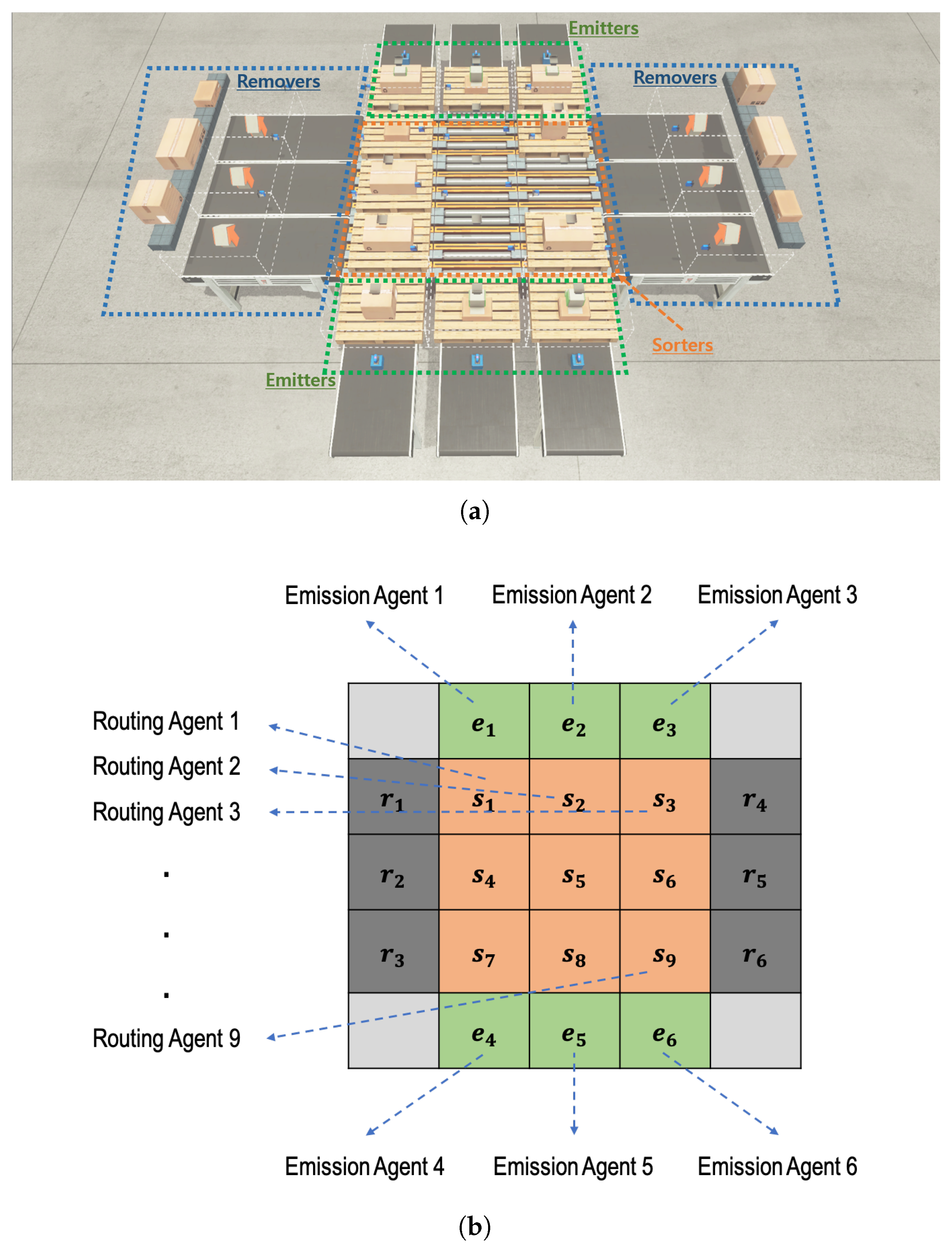
Figure 1, the system consists of three main components:
1∼4n emitters through which parcels are fed into the sortation system,
sorters by which the incoming parcels are routed (or diverted) to their specific destination, and
1∼4n removers through which parcels are unloaded from the sortation system.
The sum of the numbers of emitters and removers cannot exceed . One of the emitters is a starting point of a parcel, while one of the removers is a specific destination of a parcel. Each remover knows what type of parcels it should accept, and it determines whether the parcel has been correctly classified whenever it receives a parcel.
The sorters are deployed in the form of an grid, and each of them is controlled by an independent routing RL agent, allowing the system to have a flexible structure. On the other hand, emitters are deployed on the side of the grid, and each of them is controlled by an independent emission RL agent. The number and location of emitters are determined by the system requirements. Similarly, removers are deployed on the side of the grid, and the number and location of removers are determined by the system requirements, as well. However, there is no RL agent for a remover. This means that a remover’s behavior is determined passively by the adjacent sorter’s behavior.
Parcels are randomly fed into the
n-grid sortation system through emitters, and routing agents on each sorter decide the routing direction for each parcel on itself at every time step. In a distributed manner, the routing agents try to find the shortest path for a type of parcel from its entry emitter to its destination of a remover. In this paper, a total of six emitters are placed on the two sides of the three-grid system, a group of three emitters facing the other one, and six removers are placed in the same way on the other two sides.
Figure 1 depicts a three-grid sortation system, where there are 6 emitters (and 6 emission agents), 9 sorters (and 9 routing agents), and 6 removers.
It is assumed that 1∼6 parcels can be put into the system at the same time. Emission agents control the number of parcels put into the system every time step, in order to suppress congestion that may occur on the nine sorters. While parcels are being classified over the system, a situation may arise where two or more adjacent (emission or routing) agents’ action cannot be performed simultaneously at any time step. For example, there may be a situation where two parcels are simultaneously moved to one sorter by two adjacent routing agents or by adjacent routing and emission agents. This situation is called a collision. Later, we will explain in detail how to resolve such collisions and generate penalties for the agents that caused the collisions. The configured system has just nine sorters, and they act as buffers for parcel flow optimization. Therefore, the small number of sorters increases the risk of congestion or collision during the parcel sorting process.
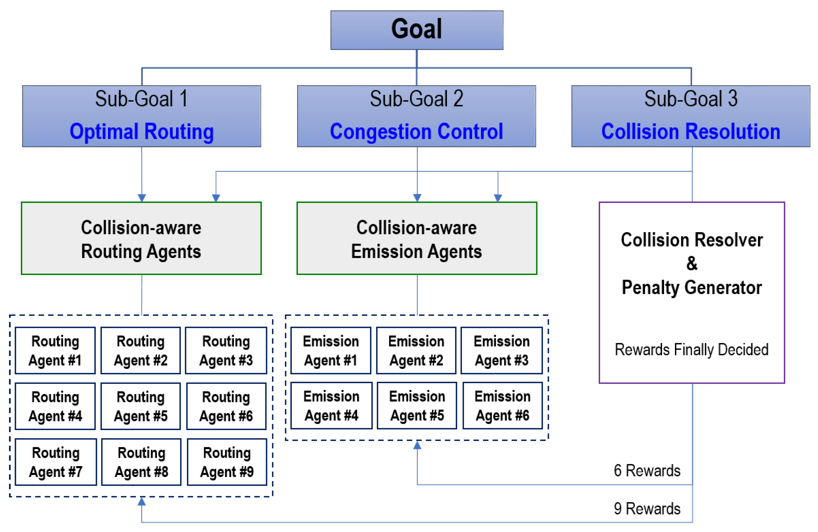
In summary, as depicted in
Figure 2, the system consists of three separate sub-goals to achieve the two ultimate objectives: (1) high accuracy and (2) high throughput.
Optimal routing: sorters should deliver parcels to their specific destination as quickly as possible.
Congestion control: emitters should control the number of incoming parcels to allow the parcels to be processed and transferred without congestion by the sorters in the system.
Collision resolution: a system-wide agent should resolve a collision caused by the actions of several routing or emission agents.
4. Design of Cooperative the Multi-Agent RL Algorithm
The proposed sortation system should solve the optimization problem for accuracy and throughput. In the system, the routing agents and the emission agents observe the current system state fully at each time step t and choose the actions based on their own policy.
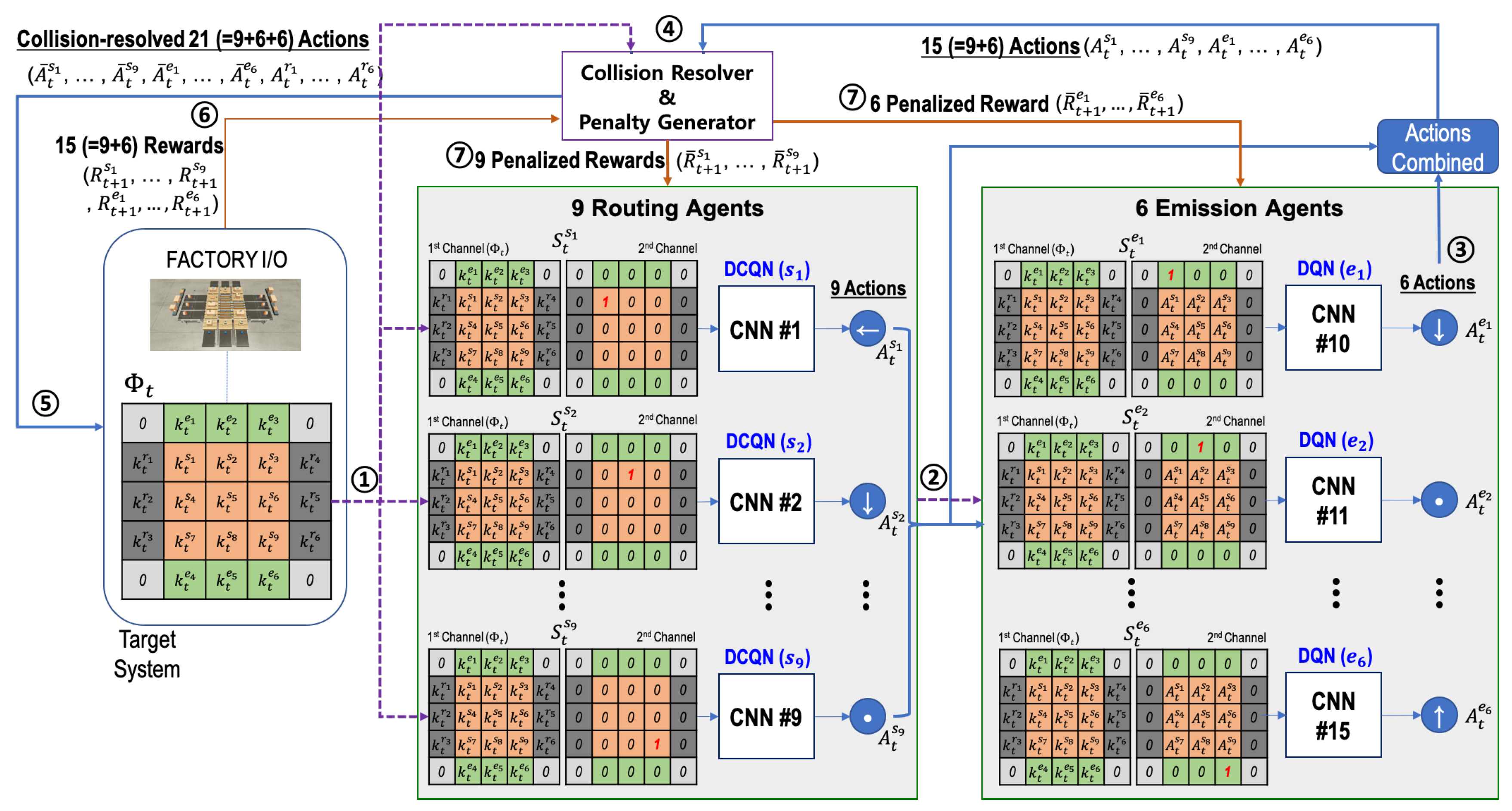
As shown in
Figure 3, for
and each time step
t, the current system’s state is represented by an
array, called parcel information
. For a sorter
(
) and an emitter
(
), the corresponding elements
and
of the array indicate the parcel type (1, 2, or 3 in our case) if a parcel is on the sorter
or the emitter
, respectively. Otherwise, the corresponding element is set to zero. For a remover
(
), the corresponding element
of the array indicates the parcel type (1, 2, or 3) that the remover
should receive. In a parcel information array
, the pixel values in the four corners are fixed at zero.
4.1. Routing Agents
There are nine sorters () in the grid system, and the routing agent connected to a sorter controls the sorter’s behavior. In this paper, sometimes, a routing agent will be also symbolized by , since any routing agent has a one-to-one correspondence with a sorter. For a time step t, the state , the action , and the reward for a routing agent are defined as follows.
The state is an two-channel image, where the first channel has the parcel information . In the second channel, all pixel values are set to zero except for the last pixel where the corresponding sorter is located. The value of the last pixel is one. The second channel serves to inform each routing agent of the agent’s location.
The action represents the selection one of five action types as the sorter ’s action. The five types are “Stop (0)”, “North (1)”, “South (2)”, “West (3)”, and “East (4)”. When a sorter performs its action, it will route the parcel to the indicated direction. If the action is zero, the corresponding sorter will do nothing. Therefore, a routing agent will select a non-stop action only when there is a parcel on the corresponding sorter. Before the selected action is performed in the target system, however, it will be altered to by the collision resolver. It should be noted that a sorter can perform the altered non-stop action even though there is no parcel on the sorter, because a sorter should perform an action to receive a parcel that an adjacent sorter sends. We will explain this in detail later.
After performing the selected action
at time step
t, the sorter
receives a reward
at the next time step
. It consists of three types of components: the “routing” reward
, the “correct classification” reward
, and the “wrong classification” reward
. Each of them has its coefficient and the range of its possible values, which are described in
Table 1. The “routing” reward
will be one when the sorter
forwards (i.e., routes) a parcel to an adjacent sorter or remover. A negative “routing” reward coefficient can lead the routing agents to minimize the number of routing behaviors, and thus, the routing path can be shortened. Therefore, this reward design helps increase the throughput measure. The “correct classification” reward
and the “wrong classification” reward
will be set to the number of correctly and wrongly classified parcels (i.e., the number of parcels correctly and wrongly arriving at six removers) at time step
, respectively. The two reward values are commonly added into
for
. It should be noted that the coefficient of the “correct classification” reward is the only positive value. Therefore, this reward design helps increase the accuracy measure. As a result, the reward
for the routing agent
is:
Before a routing agent receives the calculated reward , however, the reward will be altered to by the penalty generator. We will explain it in detail later.
4.2. Emission Agents
There are six emitters () in the system, and an emission agent connected to an emitter controls the emitter’s behavior. In this paper, sometimes, an emission agent will be also symbolized by , since any emission agent has a one-to-one correspondence with an emitter. It should be noted that the action inference of the six emission agents is proceeded after the one of the nine routing agents. For a time step t, the state , the action , and the reward for the emission agent an emission agent are defined as follows.
Like the state for the routing agents, the state is also a two-channel image, where the first channel has parcel information . On the other hand, the second channel consists of the action information inferred by the nine routing agents in the prior phase of the same time step t. That is, the nine pixels on the center of the second channel contain (). The 15 pixels on the edge of the second channel are set to zero, and the last pixel corresponding to the emitter’s location has one. The last pixel informs each emission agent of the agent’s location.
The action corresponds to the selection of one of two action types, “Stop (0)” and “Emission (1)”, as the emitter ’s action. At every time step, six parcels are placed on all six emitters. The type of parcel is randomly determined when placed on an emitter. When an emitter performs the action “Emission (1)”, the parcel on the emitter will be moved to the emitter’s adjacent sorter, and a new parcel is immediately placed on the emitter. If the action is “Stop (0)”, the corresponding emitter will do nothing, and the parcel on the emitter will be in place. Before the selected action () is performed in the target system, however, it will be altered to by the collision resolver. We will explain this in detail later.
After performing the selected action
at time step
t, the emitter agent
receives a reward
at the next time step
. It consists of two types of components: the “emission” reward
and the “in and out balance” reward
. Each of them has its coefficient and the range of its possible values, which are described in
Table 1. The “emission” reward
indicates whether or not the emitter
places its parcel on sorters at time step
. The corresponding coefficient is positive, which leads the emitters to put as many parcels as possible into the sorters. On the other hand, the “in and out balance” reward
is determined by the following equation:
In Equation (
3),
and
indicate the number of parcels fed to sorters by six emitters and the number of parcels arriving at the six removers at time step
, respectively. For all
, the same value of this reward is commonly added to
. The corresponding coefficient is negative, which leads the emitters to control the parcel congestion on the sorters. That is, if
becomes high (e.g., there is no balance between inflow and outflow of parcels), the emitters will reduce or increase the number of parcels newly placed on sorters. Therefore, this reward design helps increase the throughput measure, as well. As a result, the reward
for the emission agent
is:
Before the emission agent receives the calculated reward , however, the reward will be altered to by the penalty generator. We will explain this in detail later.
4.3. Collision Resolver and Penalty Generator
In the design of RL agents in the
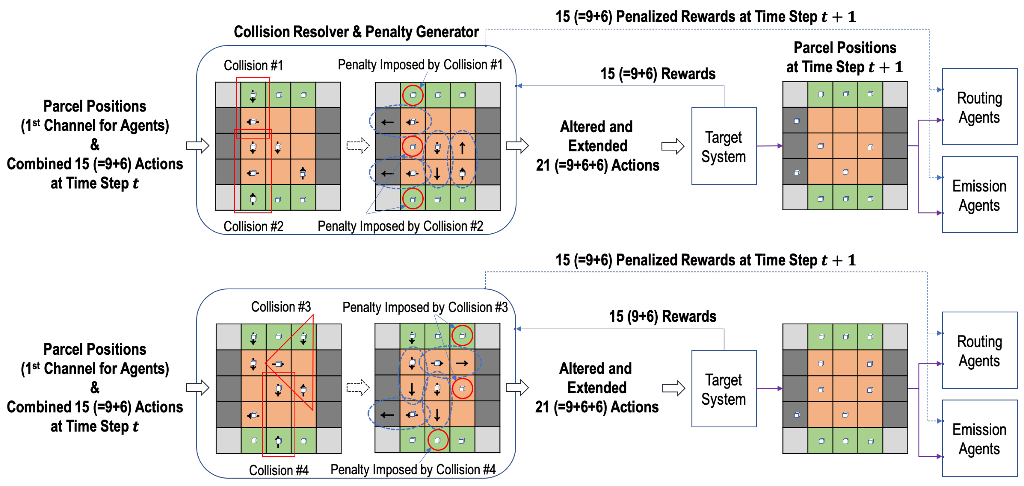
n-grid sortation system, a collision occurs when the actions selected by two or more adjacent emission or routing agents cannot be performed at the same time step.
Figure 4 describes diverse scenarios of collisions. In the figure, the locations of parcels and the actions of agents in each of the red rectangles or triangle represents a collision. Collisions #1 and #2 in the figure occur because the action directions of two or more routing and emission agents are inconsistent and cannot be performed simultaneously. Collisions #3 and #4 in the figure occur because two or more parcels are supposed to be simultaneously moved to one sorter by two or more routing and emission agents.
With the information of parcel positions and the combined actions at time step t, the collision resolver prevents such collisions. Among the actions involved in a collision, it selects the one action that will be performed at time step t and alters the rest of actions as “Stop (0)”. The selection rules are simply as follows:
The action of moving the parcel closer to the remover is selected first,
The sorter’s action takes precedence over the emitter’s action, and
If two or more actions have the same priority, one action is randomly selected.
In the first rule, the Manhattan distance is used to measure the distance between a parcel and a remover.
On the other hand, let us assume that an emission or a routing agent
is supposed to perform a non-stop action and move a parcel at time step
t. Then, the adjacent routing agent receiving the parcel that the agent
moves should perform the action of the same direction as the action’s one of the agent
. Therefore, the routing agent’s action can be altered to a non-stop action by the collision resolver, even though no parcel is located on the agent. Similarly, a remover’s action can be altered to a non-stop action for the remover to receive a parcel from a routing agent (i.e., a sorter). Actions altered in this way are denoted by the dotted ovals in
Figure 4. Finally, the collision resolver alters the original actions
and
and produces a total of 21 (=9+6+6) actions, i.e.,
for the nine sorters,
for the six emitters, and
for the six removers.
It should be noted that the routing or emission agents whose actions are altered by the collision resolver to “Stop (0)” will be penalized when they receive the reward from the target system at the next time step. In
Figure 4, the agents where the penalty is imposed are denoted by the solid red circles. The original rewards at time step
are first delivered to the penalty generator (co-located with the collision resolver), and the pre-defined penalty values are imposed in the rewards per agent depending on the selection decision of the collision resolver at time step
t. There are two kinds of collision penalty values, which are presented in
Table 1: (1)
for a routing agent
and (2)
for an emission agent
. For the two penalty values, the same negative coefficient
is used. Therefore, the original rewards
and
are changed into
and
as follows:
and the changed ones are delivered to the routing and emission agents at time step
.
4.4. Cooperative Multi-Agent RL Algorithm
In this section, we describe the proposed multi-agent RL algorithm to optimize the behavior of sorters and emitters in the n-grid sortation system. The proposed algorithm is based on DQN, so that the agents have off-policy based learning methods. The algorithm are performed as follows:
- (1)
The routing agents and the emission agent initialize their experience replay memories, action-value functions ( and ), and target action-value functions ( and ) (see Lines 1∼8 of Algorithm 1).
- (2)
An episode begins with the reset of the target system. At the reset of the target system (that is, time step
), each emitter has one parcel of a random type, and no parcel is on a sorter or a remover. The parcel information on the grid system is set to
(see Lines 10∼11 of Algorithm ① and 1 in
Figure 3).
- (3)
Based on the states configured with
and the routing agent’s location, the routing agents select their actions according to the
-greedy policy. If there is no parcel on a routing agent, its action is zero indicating “Stop” (see Lines 13∼22 of Algorithm 1 and ② in
Figure 3).
- (4)
Based on the states configured with
and the actions selected by nine routing agents, the emission agents select their actions according to the
-greedy policy (see Lines 23∼29 of Algorithm 1 and ③ in
Figure 3).
- (5)
The selected actions are delivered to the collision resolver, and it alters the actions according to the rules presented by
Section 4.3 (see Line 30∼31 of Algorithm 1 and ④ in
Figure 3).
- (6)
The altered actions at time step
t are finally performed on the target system, and the rewards at time step
are generated from it (see Lines 32∼33 of Algorithm 1 and ⑤ in
Figure 3).
- (7)
The rewards are also delivered to the penalty generator (co-located with collision resolver), and the penalized rewards are generated by it (see Lines 34∼35 of Algorithm 1 and ⑦ in
Figure 3). The penalized rewards will be delivered to the routing and emission agents. However, such delivery is not performed directly at the current time step
t, but will be performed at the optimization phase of the state-action value functions.
- (8)
The states, actions, altered actions, penalized rewards, parcel information, and episode ending information are stored in the corresponding replay memory as transition information (see Lines 36∼41 of Algorithm 1). The transition information including penalized rewards will be used when the state-action value functions are optimized. Since the actions selected by routing agents are required for the optimization task of emission agents, is configured and put into the transitions for emission agents.
- (9)
Model weight copying to the target models is performed every episodes (see Line 43 of Algorithm 1).
The optimization is performed on an episode basis, since there is not enough time to optimize their models between time steps in an episode. (Since our target system is configured on Factory I/O (i.e., a virtual simulator), the optimization can be performed even on a step basis. However, the proposed algorithm will be also executed with a real system deployed in a factory. In a real system, there will not be enough time to perform the optimization on a step basis.)
To determine whether an episode ends, two numbers, L and M, are tracked as follows:
L: the total number of parcels arriving at a remover (i.e., the number of parcels classified) and
M: the number of parcel moves by any one sorter.
In addition, there are two different thresholds
and
, and if
or
in the course of an episode, the episode comes to end. When the selected actions are performed at time step
t, the target system notifies the agents of the end of the episode through the Boolean variable
(see Line 33 of Algorithm 1).
| Algorithm 1: The proposed multi-agent RL algorithm (Γ: target system, Ω: collision resolver and penalty generator, ϵ ∈ [0, 1]: exploration threshold). |
 |
On the other hand, the state-action value function optimization is performed at each routing agent () as follows:
- (1)
A routing agent samples a random mini-batch of K transitions from its replay memory (see Line 2 of Algorithm 2).
- (2)
For each transition, the routing agent should get the next routing agent or remover , which its action is bound to, because the target value for the loss equation at time step t comes from (see Line 4 of Algorithm 2).
- (3)
The action moving a parcel to
was selected by
according to its policy (i.e.,
-greedy at
) at the current time step
t. At time step
, after one step progresses, the moving parcel passes to
. Therefore, the target value for the loss equation should be provided by
(see Line 9 of Algorithm 2). We call this strategy the deep chain Q network (DCQN). The strategy is similar to the one of Q-routing [
32], which is a well-known RL algorithm in the field of computer network where a node needs to select its adjacent node where the node sends a network packet so that the node delivers the packet to its final destination as soon as possible.
By Algorithm 2, the routing agents learn the optimal routing paths for parcels. However, when routing agents find the optimal routing paths, those may change each time according to the type of parcels and their entry order. Therefore, the routing agents need to collaborate with other agents while predicting future invisible situations. This collaboration is achieved to some extent by the rewards
and
common to all routing agents.
| Algorithm 2: optimization for routing agent (). |
 |
Parcel loads imposed on routing agents are different each time, and congestion can occur on the grid system. Such congestion can be prevented by emission agents. The emission agents adjust the number of the emitted parcels by predicting the overall flow of parcels through the transition information of the mini-batch and the included reward value. The state-action value function optimization is performed at each emission agent () as follows:
- (1)
The transitions in a mini-batch are sampled sequentially (see Line 2 of Algorithm 3).
- (2)
The target value for the loss equation at time step t is calculated just from (1) the reward of the next time step and (2) the maximum state-action value for the emission agent at the next time step (see Lines 7∼8 of Algorithm 3). For the next time step , should be configured with the actions of the routing actions at time step . Therefore, The transitions in a mini-batch should be sampled sequentially.
In the reward
of each transition,
induces an emitter
to release its parcel into the adjacent sorter. On the other hand,
is common to all emission agents, and the collaboration between emission agents is achieved to some extent by this reward.
| Algorithm 3: optimization for routing agent (). |
 |
5. Performance Evaluation
In this section, we evaluate the performance of the proposed multi-agent RL algorithm on the three-grid sortation system implemented on Factory I/O. We also present that the well-trained collaborative RL agents could optimize their performance effectively.
5.1. Training Details and Performance Measure
We performed our experiments on the three-grid sortation system, the configuration of which is explained in
Figure 1 in
Section 3. In the target system, with the collision resolver, the proposed two types of agents worked together to sort and move the parcels as fast as possible and prevent parcel congestion through continuous learning. Training was performed on an episode basis, and during an episode, an unlimited number of parcels of three types were fed by the emitters at random. However, we set
to 512, so that an episode came to end when 512 parcels were classified on removers. We also set
to 1024, so that an episode also came to end when any one sorter moved parcels more than 1024 times. At this time, all the sorters obtained much negative routing reward
, so that it could prevent two or more sorters from sending and receiving the same parcels many times.
In this study, a new performance indicator, called the sorting performance index (SPI), is presented to measure how well the routing and emission agents achieved the two given goals, high accuracy and high throughput, together. For an episode
e,
is given by the following equation:
where
indicates the total time steps elapsed during episode
e. The two values
and
represent the numbers of parcels classified correctly and wrongly at time step
t, respectively (
. As shown in
Table 1, the two values are components of the reward delivered to a routing agent, and by using Equation (
3),
. Therefore,
indicates the average correct classification rate per time step, while
indicates the average wrong classification rate per time step. The SPI value was obtained by the difference between the two rates for an episode. It was also divided by the number of removers (=6) for normalization, so that it was between
and
.
In the learning experiment, a total of 2700 episodes were performed repeatedly. We used -greedy as the behavior sampling policy for routing and emission agents, and the value was gradually decreased from to across all the episodes. Finally, the step size (learning rate) was set to 0.0001, the discount factor to 0.99, and the episode interval for weight copying to five. It took five hours to finish the learning experiment on the GEFORCE RTX 2080 Ti GPU. We conducted seven experiments and collected the average, the maximum, and the minimum values of the performance measures for every episode.
5.2. Results
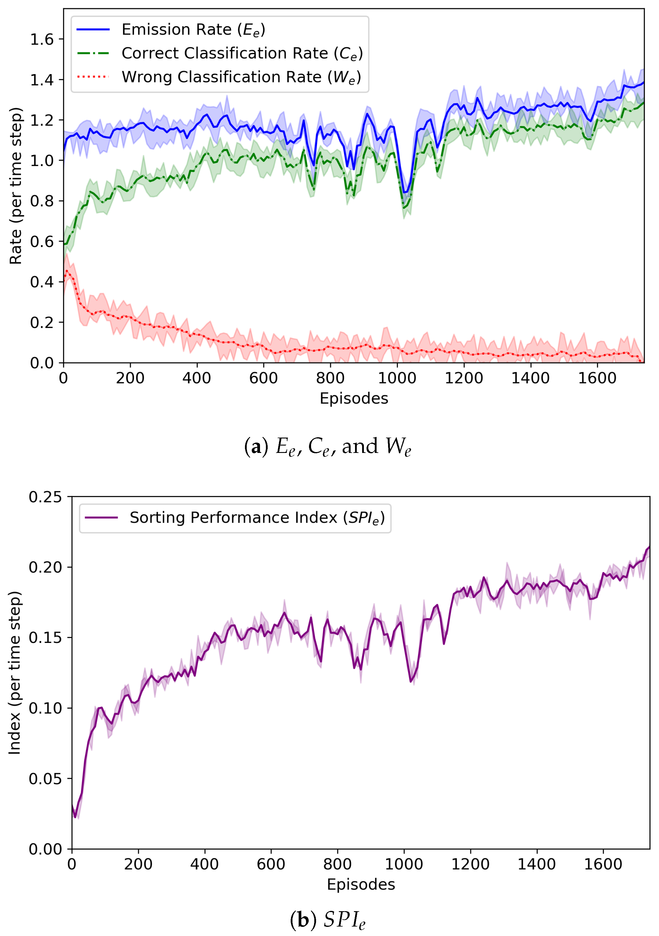
Figure 5 reveals the change of the average emission rate
, average correct classification rate
, average wrong classification rate
, and sorting performance index
for each episode
e. By using Equation (
3), the emission rate
is simply defined as:
It was found that the emission rate did not become high (it was up to 1.4). The emission agents continuously monitored the behavior of the routing agents, analyzed the given rewards, and controlled the amount of parcels fed to sorters. Since there were just nine sorters in the form of a 3 × 3 grid, a large number of parcels could not be fed into the sorters. From the low emission rate, we could know that the emission agents were trained well and their behavior was appropriate.
The emission agents also tried to balance the number of parcels fed to the sorters with the number of parcels removed by the removers. That is, they tried to make the two values, and , equal. Overall, was lower than . This was because if (=512) parcels were classified by agents or (=1024) times of moves were performed by a sorter, an episode came to end even though a number of unclassified parcels still remained on the sorters.
As shown in
Figure 5a, at the beginning of the learning experiment,
and
were almost similar, but as learning was repeated,
tended to decrease and
to increase. From these results, we could know that the routing agents worked together to find the correct routing paths for the parcels and the emission agents had the ability to control the number of parcels fed by themselves well.
In
Figure 5b, the change of
is also depicted. At the 1780th episode,
was calculated as the largest value, 0.21. It is noted that
was almost 0.0 at that episode. Whenever the
value hit the highest point, the RL policy model being trained was saved, and we finally obtained the best models of agents. These results proved that the proposed cooperative multi-agent RL algorithm was effective for the
n-grid sortation system to sort the parcels as fast as possible.
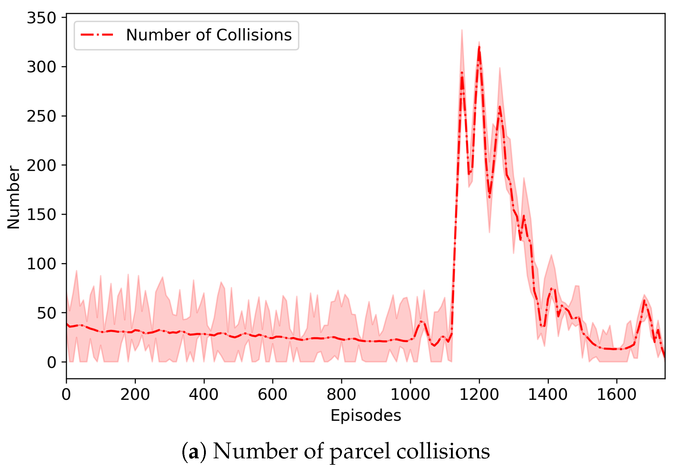
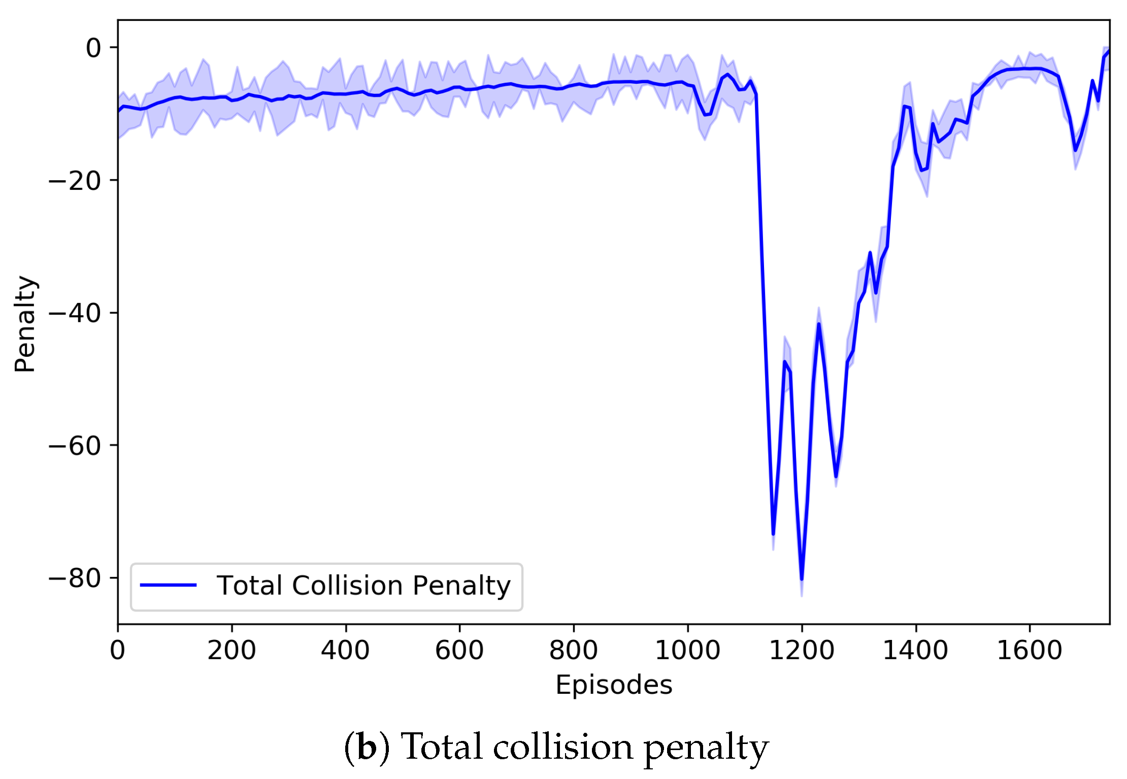
Figure 6 depicts the change of the number of parcel collisions that may occur in our three-grid sortation system and also represents the change of the total collision penalty imposed on routing and emission agents. In the system, parcels were generated randomly regardless of their type and order, and they should be classified to their designated removers. However, the number of sorters was relatively small, so that there were not enough buffers where parcels moved and were located. This directly led to numerous collisions (or congestion) of parcels. Through repeated learning, however, routing agents were increasingly good at finding the optimal route for parcels, and the emission agents were also increasingly good at controlling the congestion. Nevertheless, routing and emission agents may select their actions that can cause collisions of parcels. In the proposed system, the collision resolver changed them, so that the collision-resolved actions were finally performed on the system. Instead, the collision penalties were imposed as penalized rewards on the routing and emission agents causing the collisions. According to our experiments, the number of collisions varied largely during some episodes, but after those, the number of collisions became very low. It can be seen from
Figure 6 that a similar situation occurred. The number of collisions began to vary from about 1000 episodes, and thus, the total collision penalty was changed accordingly. It is noted that the episode (i.e., the 1780th episode) where the best model was saved was the one where the number of collisions almost became zero after the number of collisions was varied.
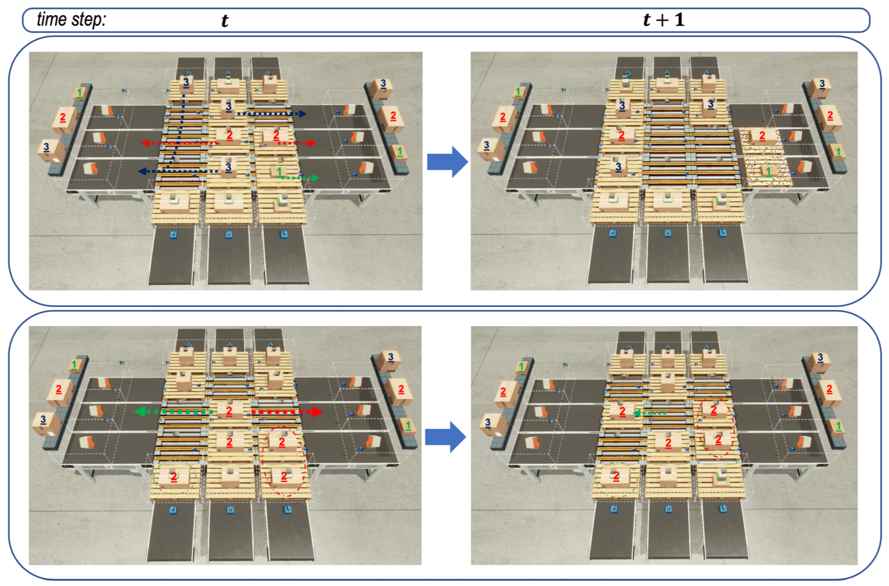
Finally,
Figure 7 depicts the behavior of emitters and sorters that were controlled by the well-trained RL agents. In fact, the well-trained RL agents had the models saved at the 1780th episode. The figure shows the behaviors between two successive time steps
t and
on the left and right sub-figures, so that we can try to expect the next behaviors of emitters and sorters from the left sub-figure and check the behaviors selected by emitters and sorters from the right sub-figure. By expecting and checking from two sub-figures, we could know that the agents performed their actions well, as expected.
6. Conclusions
In this paper, we designed an n-grid sortation system that could be used in the intralogistics industry and developed a collaborative multi-agent RL algorithm to control the behavior of emitters or sorters in the system. The system’s goal had two sub-goals: (1) high accuracy and (2) high throughput; that is, the parcels fed into sorters should be routed to the removers correctly and quickly. There were two types of RL agents, emission agents and routing agents, and they were trained to solve the given multi-objective optimization problem together. We described the agents’ learning performance by depicting the changes of the SPI value, as well as the emission rate, the correct classification rate, and the wrong classification rate. We also represented the changes of the number of parcel collisions and of the total collision penalty imposed on routing and emission agents. The RL models of agents were saved whenever the SPI value hit the highest point, so that we could get the best models after the RL learning was over. From the learning results, we could know that the well-trained routing and emission agents could achieve the given multiple objectives effectively. In particular, the routing agents finally learned to route the parcels through their optimal path, and the emission agents finally learned to control the parcel congestion on the sorters.
In future work, we will design a more flexible sortation system so that the formation of the system is not limited to a grid shape. The routing and emission agents should be designed again to support such a flexible formation. In addition to that, we will provide a new design of the RL agents to allow them to resolve the parcel collisions by themselves without the aid of the independent collision resolver.

 ,
, 


