Color Image Generation from LiDAR Reflection Data by Using Selected Connection UNET


Abstract
1. Introduction
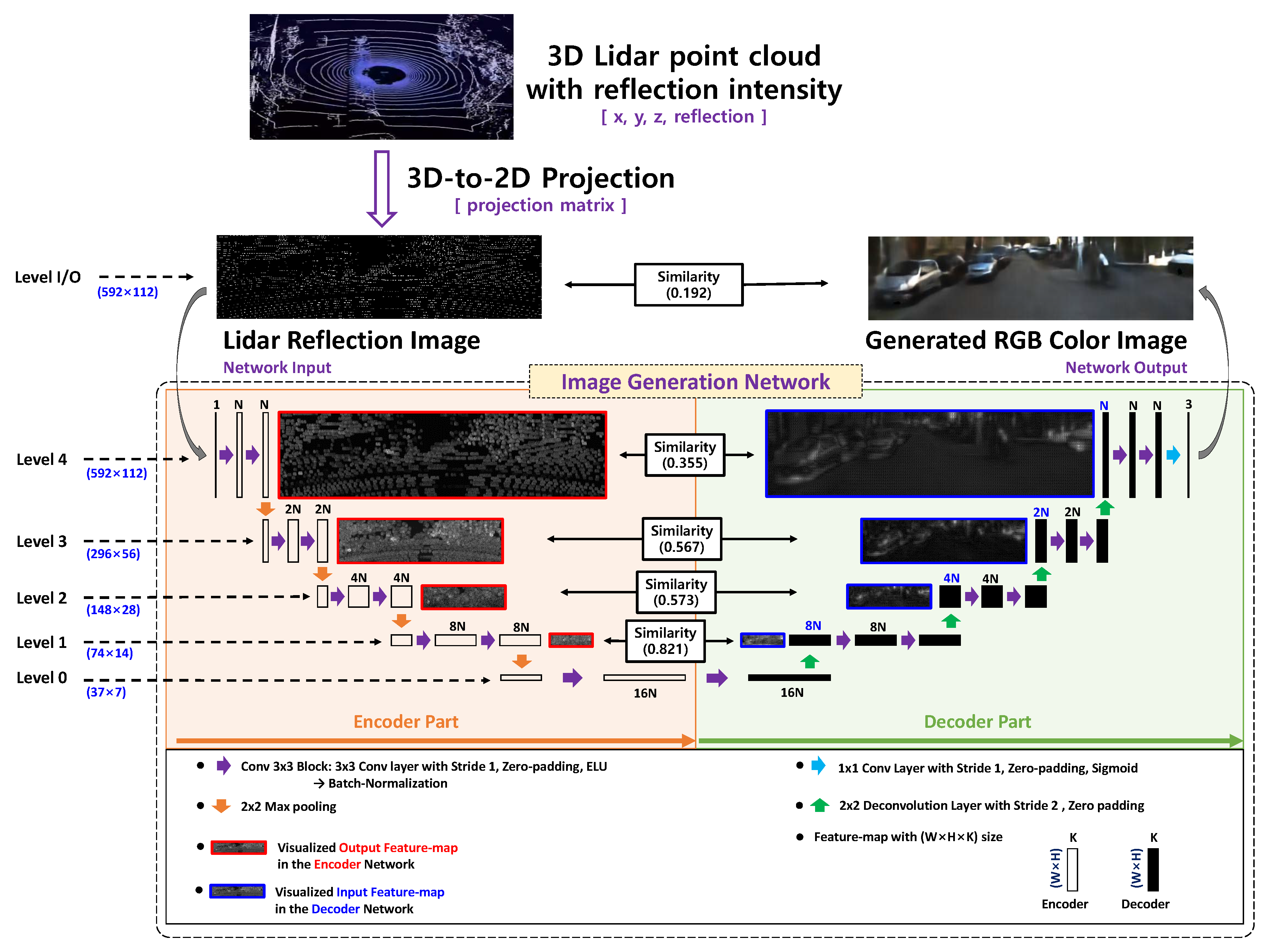
2. Proposed Method
2.1. Sparseness and Similarity of ED-FCN
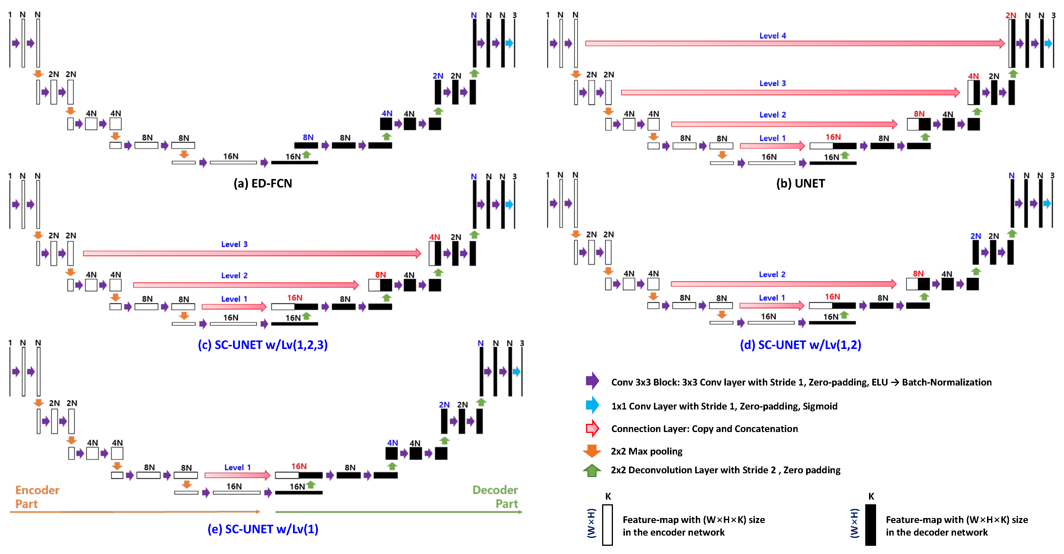
2.2. Proposed Network Architectures
2.3. Training and Inference Processes
3. Simulation Environment and Results
3.1. Simulation Environment
3.2. Performance of the Proposed SC-UNET-Based Architectures
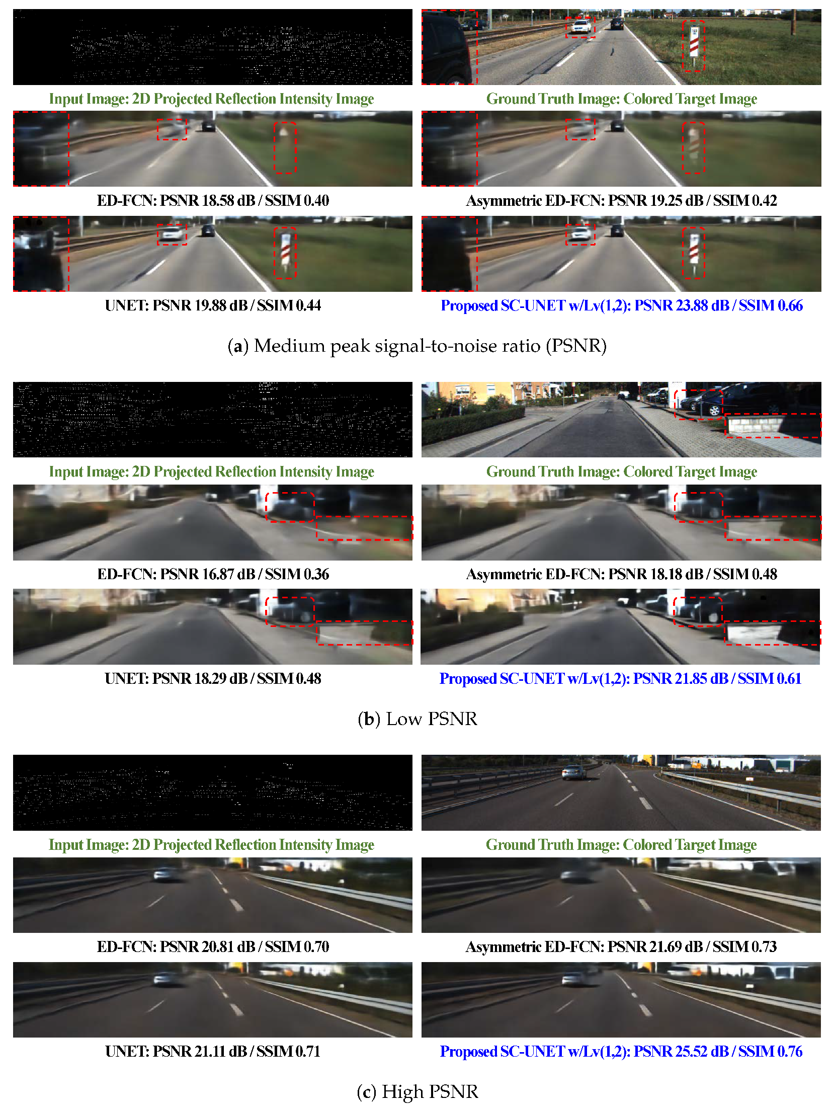
3.3. Inference Examples
4. Conclusions
Author Contributions
Funding
Conflicts of Interest
Appendix A. Analysis of Sparseness Using Receptive Field

| Level (L) | P | B | ||
|---|---|---|---|---|
| 4 | 0 | 2 | 0 | 2 |
| 3 | 1 | 2 | 1 | 4 |
| 2 | 1 | 2 | 2 | 6 |
| 1 | 1 | 2 | 3 | 8 |
| 0 | 1 | 2 | 4 | 10 |

| Level (L) | Size of Receptive Field | Sparseness (%) |
|---|---|---|
| 4 | 5 × 5 | 42.63 |
| 3 | 18 × 18 | 8.72 |
| 2 | 52 × 52 | 0.92 |
| 1 | 136 × 136 | 0.00 |
References
- Reymann, C.; Lacroix, S. Improving LiDAR point cloud classification using intensities and multiple echoes. In Proceedings of the 2015 IEEE/RSJ International Conference on Intelligent Robots and Systems (IROS), Hamburg, Germany, 28 September–2 October 2015; pp. 5122–5128. [Google Scholar]
- Gao, H.; Cheng, B.; Wang, J.; Li, K.; Zhao, J.; Li, D. Object Classification Using CNN-Based Fusion of Vision and LIDAR in Autonomous Vehicle Environment. IEEE Trans. Ind. Informat. 2018, 14, 4224–4231. [Google Scholar] [CrossRef]
- Yu, L.; Li, X.; Fu, C.W.; Cohen-Or, D.; Heng, P.A. PU-Net: Point Cloud Upsampling Network. In Proceedings of the Conference on Computer Vision and Pattern Recognition, Salt Lake City, UT, USA, 18–23 June 2018; pp. 2790–2799. [Google Scholar]
- Wurm, K.M.; Kümmerle, R.; Stachniss, C.; Burgard, W. Improving robot navigation in structured outdoor environments by identifying vegetation from laser data. In Proceedings of the 2009 IEEE/RSJ International Conference on Intelligent Robots and Systems, St. Louis, MO, USA, 11–15 October 2009; pp. 1217–1222. [Google Scholar]
- Gao, Y.; Zhong, R.; Tang, T.; Wang, L.; Liu, X. Automatic extraction of pavement markings on streets from point cloud data of mobile LiDAR. Meas. Sci. Technol. 2017, 28, 085203. [Google Scholar] [CrossRef]
- McManus, C.; Furgale, P.; Barfoot, T.D. Towards appearance-based methods for lidar sensors. In Proceedings of the 2011 IEEE International Conference on Robotics and Automation, Shanghai, China, 9–13 May 2011; pp. 1930–1935. [Google Scholar]
- Tatoglu, A.; Pochiraju, K. Point cloud segmentation with LIDAR reflection intensity behavior. In Proceedings of the 2012 IEEE International Conference on Robotics and Automation, Saint Paul, MN, USA, 14–18 May 2012; pp. 786–790. [Google Scholar]
- Dewan, A.; Oliveira, G.L.; Burgard, W. Deep semantic classification for 3D LiDAR data. In Proceedings of the 2017 IEEE/RSJ International Conference on Intelligent Robots and Systems (IROS), Vancouver, BC, Canada, 24–28 September 2017; pp. 3544–3549. [Google Scholar]
- Radi, H.; Ali, W. VolMap: A Real-time Model for Semantic Segmentation of a LiDAR surrounding view. arXiv 2019, arXiv:1906.11873. [Google Scholar]
- Kim, H.K.; Yoo, K.Y.; Park, J.H.; Jung, H.Y. Deep Learning Based Gray Image Generation from 3D LiDAR Reflection Intensity. IEMEK J. Embed. Syst. Appl. 2019, 14, 1–9. [Google Scholar]
- Milz, S.; Simon, M.; Fischer, K.; Pöpperl, M. Points2Pix: 3D Point-Cloud to Image Translation using conditional Generative Adversarial Networks. arXiv 2019, arXiv:1901.09280. [Google Scholar]
- Kim, H.K.; Yoo, K.Y.; Park, J.H.; Jung, H.Y. Asymmetric Encoder-Decoder Structured FCN Based LiDAR to Color Image Generation. Sensors 2019, 19, 4818. [Google Scholar] [CrossRef] [PubMed]
- Zhou, Z.; Siddiquee, M.M.R.; Tajbakhsh, N.; Liang, J. Unet++: A nested u-net architecture for medical image segmentation. In Deep Learning in Medical Image Analysis and Multimodal Learning for Clinical Decision Support; Springer: Cham, Switzerland, 2018; pp. 3–11. [Google Scholar]
- Sun, Y.; Zuo, W.; Liu, M. Rtfnet: Rgb-thermal fusion network for semantic segmentation of urban scenes. IEEE Robot. Autom. Lett. 2019, 4, 2576–2583. [Google Scholar] [CrossRef]
- Long, J.; Shelhamer, E.; Darrell, T. Fully convolutional networks for semantic segmentation. In Proceedings of the IEEE conference on computer vision and pattern recognition, Boston, MA, USA, 7–12 June 2015; pp. 3431–3440. [Google Scholar]
- Jiang, N.; Wang, L. Quantum image scaling using nearest neighbor interpolation. Quantum Inf. Process. 2015, 14, 1559–1571. [Google Scholar] [CrossRef]
- Babak, O.; Deutsch, C.V. Statistical approach to inverse distance interpolation. Stoch. Environ. Res. Risk Assess. 2009, 23, 543–553. [Google Scholar] [CrossRef]
- Isola, P.; Zhu, J.; Zhou, T.; Efros, A.A. Image-to-Image Translation with Conditional Adversarial Networks. In Proceedings of the 2017 IEEE Conference on Computer Vision and Pattern Recognition, Honolulu, HI, USA, 21–26 July 2017; pp. 5967–5976. [Google Scholar]
- Noh, H.; Hong, S.; Han, B. Learning deconvolution network for semantic segmentation. In Proceedings of the 2015 IEEE International Conference on Computer Vision (ICCV), Santiago, Chile, 7–13 December 2015; pp. 1520–1528. [Google Scholar]
- Badrinarayanan, V.; Kendall, A.; Cipolla, R. Segnet: A deep convolutional encoder-decoder architecture for image segmentation. IEEE Trans. Pattern Anal. Mach. Intell. 2017, 39, 2481–2495. [Google Scholar] [CrossRef]
- Kim, H.K.; Yoo, K.Y.; Park, J.H.; Jung, H.Y. Traffic light recognition based on binary semantic segmentation network. Sensors 2019, 19, 1700. [Google Scholar] [CrossRef] [PubMed]
- Ronneberger, O.; Fischer, P.; Brox, T. U-net: Convolutional networks for biomedical image segmentation. In Medical Image Computing and Computer-Assisted Intervention—MICCAI 2015; Springer: Cham, Switzerland, 2015; pp. 234–241. [Google Scholar]
- Liang, D.; Pan, J.; Yu, Y.; Zhou, H. Concealed object segmentation in terahertz imaging via adversarial learning. Optik 2019, 185, 1104–1114. [Google Scholar] [CrossRef]
- Liu, H.; Hu, Z.; Mian, A.; Tian, H.; Zhu, X. A new user similarity model to improve the accuracy of collaborative filtering. Knowl. Based Syst. 2014, 56, 156–166. [Google Scholar] [CrossRef]
- Huang, Z.; Wang, N. Like What You Like: Knowledge Distill via Neuron Selectivity Transfer. arXiv 2017, arXiv:1707.01219. [Google Scholar]
- Clevert, D.A.; Unterthiner, T.; Hochreiter, S. Fast and accurate deep network learning by exponential linear units (elus). arXiv 2015, arXiv:1511.07289. [Google Scholar]
- Ioffe, S.; Szegedy, C. Batch Normalization: Accelerating Deep Network Training by Reducing Internal Covariate Shift. arXiv 2015, arXiv:1502.03167. [Google Scholar]
- Zeiler, M.D.; Krishnan, D.; Taylor, G.W.; Fergus, R. Deconvolutional networks. In Proceedings of the 2010 IEEE Computer Society Conference on Computer Vision and Pattern Recognition, San Francisco, CA, USA, 13–18 June 2010. [Google Scholar]
- Karlik, B.; Olgac, A.V. Performance analysis of various activation functions in generalized MLP architectures of neural networks. Int. J. Intell. Syst. 2011, 1, 111–122. [Google Scholar]
- Kingma, D.P.; Ba, J. Adam: A Method for Stochastic Optimization. arXiv 2014, arXiv:1412.6980. [Google Scholar]
- Prechelt, L. Automatic early stopping using cross validation: Quantifying the criteria. Neural Netw. 1998, 11, 761–767. [Google Scholar] [CrossRef]
- Geiger, A.; Lenz, P.; Stiller, C.; Urtasun, R. Vision meets robotics: The KITTI dataset. Int. J. Robot. Res. 2013, 32, 1231–1237. [Google Scholar] [CrossRef]
- Rodriguez, J.D.; Perez, A.; Lozano, J.A. Sensitivity Analysis of k-Fold Cross Validation in Prediction Error Estimation. IEEE Trans. Pattern Anal. Mach. Intell. 2010, 32, 569–575. [Google Scholar] [CrossRef] [PubMed]
- Murty, M.N.; Devi, V.S. Pattern Recognition: An Algorithmic Approach; Springer: London, UK, 2011. [Google Scholar]
- Hore, A.; Ziou, D. Image Quality Metrics: PSNR vs. SSIM. In Proceedings of the 2010 20th International Conference on Pattern Recognition (ICPR), Istanbul, Turkey, 23–26 August 2010; pp. 2366–2369. [Google Scholar]
- Abadi, M.; Barham, P.; Chen, J.; Chen, Z.; Davis, A.; Dean, J.; Devin, M.; Ghemawat, S.; Irving, G.; Isard, M.; et al. Tensorflow: A system for large-scale machine learning. In Proceedings of the 12th USENIX Symposium on Operating Systems Design and Implementation, Savannah, GA, USA, 2–4 November 2016; pp. 265–283. [Google Scholar]
- Keras. Available online: https://keras.io (accessed on 8 October 2019).
- LeCun, Y.; Bengio, Y. Convolutional networks for images, speech, and time series. In The Handbook of Brain Theory and Neural Networks; MIT Press: Cambridge, MA, USA, 1995. [Google Scholar]
- Dumoulin, V.; Visin, F. A guide to convolution arithmetic for deep learning. arXiv 2016, arXiv:1603.07285. [Google Scholar]


| Level | The Number of Weights in the Encoder Feature Map | Size of Receptive Field | Sparseness (%) | Similarity |
|---|---|---|---|---|
| Level 4 | 66,304N (592 × 112 ) | 5 × 5 | 42.63 | 0.355 |
| Level 3 | 33,152N (296 × 56 × 2N) | 18 × 18 | 8.72 | 0.567 |
| Level 2 | 16,576N (148 × 28 × 4N) | 52 × 52 | 0.92 | 0.573 |
| Level 1 | 8288N (74 × 14 × 8 N) | 136 × 136 | 0.00 | 0.821 |
| The Number of Filters in the First Convolution Layer | Network Architecture | The Number of Weights [ea.] | Average Processing Time [ms] | Dataset in [12] | The 5-Fold Cross Validation | ||
|---|---|---|---|---|---|---|---|
| PSNR | SSIM | PSNR [AVR. (STD.)] | SSIM [AVR. (STD.)] | ||||
| ED-FCN | 1,747,955 | 4.47 | 17.98 | 0.43 | 17.90 (2.12) | 0.43 (0.14) | |
| UNET | 1,943,795 | 4.88 | 18.01 | 0.43 | 17.92 (2.88) | 0.43 (0.19) | |
| SC-UNET w/Lv(1,2,3) | 1,941,491 | 4.53 | 18.04 | 0.44 | 18.01 (2.11) | 0.44 (0.17) | |
| SC-UNET w/Lv(1,2) | 1,932,275 | 4.50 | 18.17 | 0.45 | 18.10 (2.91) | 0.44 (0.15) | |
| SC-UNET w/Lv(3,4) | 1,759,475 | 4.48 | 17.99 | 0.42 | 17.82 (2.15) | 0.41 (0.17) | |
| SC-UNET w/Lv(4) | 1,750,259 | 4.48 | 17.99 | 0.43 | 17.90 (2.11) | 0.43 (0.18) | |
| SC-UNET w/Lv(3) | 1,757,171 | 4.48 | 18.01 | 0.43 | 17.94 (2.19) | 0.43 (0.17) | |
| SC-UNET w/Lv(2) | 1,784,819 | 4.48 | 18.08 | 0.44 | 17.99 (2.18) | 0.44 (0.18) | |
| SC-UNET w/Lv(1) | 1,895,411 | 4.49 | 18.09 | 0.44 | 18.08 (2.82) | 0.44 (0.17) | |
| ED-FCN | 6,991,331 | 8.97 | 18.65 | 0.47 | 18.55 (2.28) | 0.44 (0.11) | |
| UNET | 7,765,475 | 9.49 | 18.88 | 0.49 | 18.81 (2.27) | 0.49 (0.11) | |
| SC-UNET w/Lv(1,2,3) | 7,018,979 | 9.28 | 18.90 | 0.48 | 18.76 (2.28) | 0.46 (0.11) | |
| SC-UNET w/Lv(1,2) | 7,719,395 | 9.34 | 18.93 | 0.49 | 18.87 (2.41) | 0.48 (0.11) | |
| SC-UNET w/Lv(3,4) | 6,982,115 | 8.87 | 18.69 | 0.48 | 18.56 (2.23) | 0.47 (0.11) | |
| SC-UNET w/Lv(4) | 7,028,195 | 9.19 | 18.71 | 0.48 | 18.62 (2.28) | 0.47 (0.11) | |
| SC-UNET w/Lv(3) | 7,571,939 | 9.31 | 18.88 | 0.49 | 18.76 (2.28) | 0.48 (0.11) | |
| SC-UNET w/Lv(2) | 7,129,571 | 9.31 | 18.91 | 0.49 | 18.79 (2.31) | 0.48 (0.11) | |
| SC-UNET w/Lv(1) | 7,756,259 | 9.40 | 18.91 | 0.49 | 18.83 (2.39) | 0.49 (0.11) | |
| ED-FCN | 15,702,483 | 14.16 | 18.91 | 0.49 | 18.73 (2.20) | 0.47 (0.12) | |
| UNET | 17,465,043 | 15.29 | 19.14 | 0.50 | 19.06 (2.29) | 0.50 (0.11) | |
| SC-UNET w/Lv(1,2,3) | 17,444,307 | 15.12 | 19.98 | 0.55 | 19.88 (2.29) | 0.55 (0.11) | |
| SC-UNET w/Lv(1,2) | 17,361,363 | 15.01 | 21.78 | 0.58 | 21.76 (2.49) | 0.58 (0.11) | |
| SC-UNET w/Lv(3,4) | 15,806,163 | 14.74 | 19.07 | 0.50 | 18.94 (2.31) | 0.49 (0.11) | |
| SC-UNET w/Lv(4) | 15,723,219 | 14.34 | 18.99 | 0.49 | 18.86 (2.29) | 0.48 (0.12) | |
| SC-UNET w/Lv(3) | 15,785,427 | 14.91 | 19.08 | 0.50 | 18.98 (2.28) | 0.49 (0.11) | |
| SC-UNET w/Lv(2) | 16,034,259 | 14.95 | 20.12 | 0.55 | 19.96 (2.52) | 0.55 (0.12) | |
| SC-UNET w/Lv(1) | 17,029,587 | 14.96 | 20.16 | 0.55 | 20.02 (2.68) | 0.55 (0.11) | |
| ED-FCN | 27,909,059 | 21.43 | 19.01 | 0.48 | 18.98 (2.21) | 0.47 (0.11) | |
| UNET | 31,042,499 | 23.13 | 19.37 | 0.52 | 19.27 (2.22) | 0.51 (0.12) | |
| SC-UNET w/Lv(1,2,3) | 31,005,635 | 22.87 | 20.29 | 0.56 | 19.89 (2.21) | 0.56 (0.11) | |
| SC-UNET w/Lv(1,2) | 30,858,179 | 22.71 | 23.42 | 0.68 | 23.15 (2.61) | 0.67 (0.12) | |
| SC-UNET w/Lv(3,4) | 28,093,379 | 22.30 | 19.16 | 0.51 | 19.08 (2.32) | 0.50 (0.13) | |
| SC-UNET w/Lv(4) | 27,945,923 | 21.69 | 19.08 | 0.48 | 18.92 (2.21) | 0.48 (0.12) | |
| SC-UNET w/Lv(3) | 28,056,515 | 22.56 | 19.31 | 0.51 | 19.16 (2.28) | 0.50 (0.12) | |
| SC-UNET w/Lv(2) | 28,498,883 | 22.62 | 21.83 | 0.58 | 21.60 (2.52) | 0.58 (0.12) | |
| SC-UNET w/Lv(1) | 30,268,355 | 22.63 | 22.29 | 0.62 | 22.01 (2.65) | 0.61 (0.12) | |
| - | Asymmetric ED-FCN [12] | 3,350,243 | 7.74 | 19.38 | 0.50 | 19.28 (2.18) | 0.50 (0.11) |
© 2020 by the authors. Licensee MDPI, Basel, Switzerland. This article is an open access article distributed under the terms and conditions of the Creative Commons Attribution (CC BY) license (http://creativecommons.org/licenses/by/4.0/).
Share and Cite
Kim, H.-K.; Yoo, K.-Y.; Jung, H.-Y. Color Image Generation from LiDAR Reflection Data by Using Selected Connection UNET. Sensors 2020, 20, 3387. https://doi.org/10.3390/s20123387
Kim H-K, Yoo K-Y, Jung H-Y. Color Image Generation from LiDAR Reflection Data by Using Selected Connection UNET. Sensors. 2020; 20(12):3387. https://doi.org/10.3390/s20123387
Chicago/Turabian StyleKim, Hyun-Koo, Kook-Yeol Yoo, and Ho-Youl Jung. 2020. "Color Image Generation from LiDAR Reflection Data by Using Selected Connection UNET" Sensors 20, no. 12: 3387. https://doi.org/10.3390/s20123387
APA StyleKim, H.-K., Yoo, K.-Y., & Jung, H.-Y. (2020). Color Image Generation from LiDAR Reflection Data by Using Selected Connection UNET. Sensors, 20(12), 3387. https://doi.org/10.3390/s20123387