Smart Bioimpedance Spectroscopy Device for Body Composition Estimation

 , , , , , and
Abstract
:1. Introduction
2. Materials and Methods
2.1. Monitoring System Architecture
- Smart bioimpedance device: It is a portable device capable of carrying out bioimpedance measurements in multiple configurable frequencies, processing the data to obtain the modulus and the bioimpedance phase in each of the frequencies, and transmitting the processed information wirelessly.
- Personal monitoring device (master): Data acquired by the smart bioimpedance device are wirelessly transmitted to a smartphone that performs a second processing to estimate the BC from the identification of parameters of a three-dispersion bioimpedance model. Besides, by adapting the model described in [3] the personal monitoring device provides an estimation of the following parameters: extracellular water (ECW), intracellular water (ICW), total body water (TBW), fat mass (FM) and fat free mass (FFM). The processing algorithms are implemented in Java by a mobile application for Android operating system. This device also serves as user interface and communications gateway for data storage and remote management of the information.
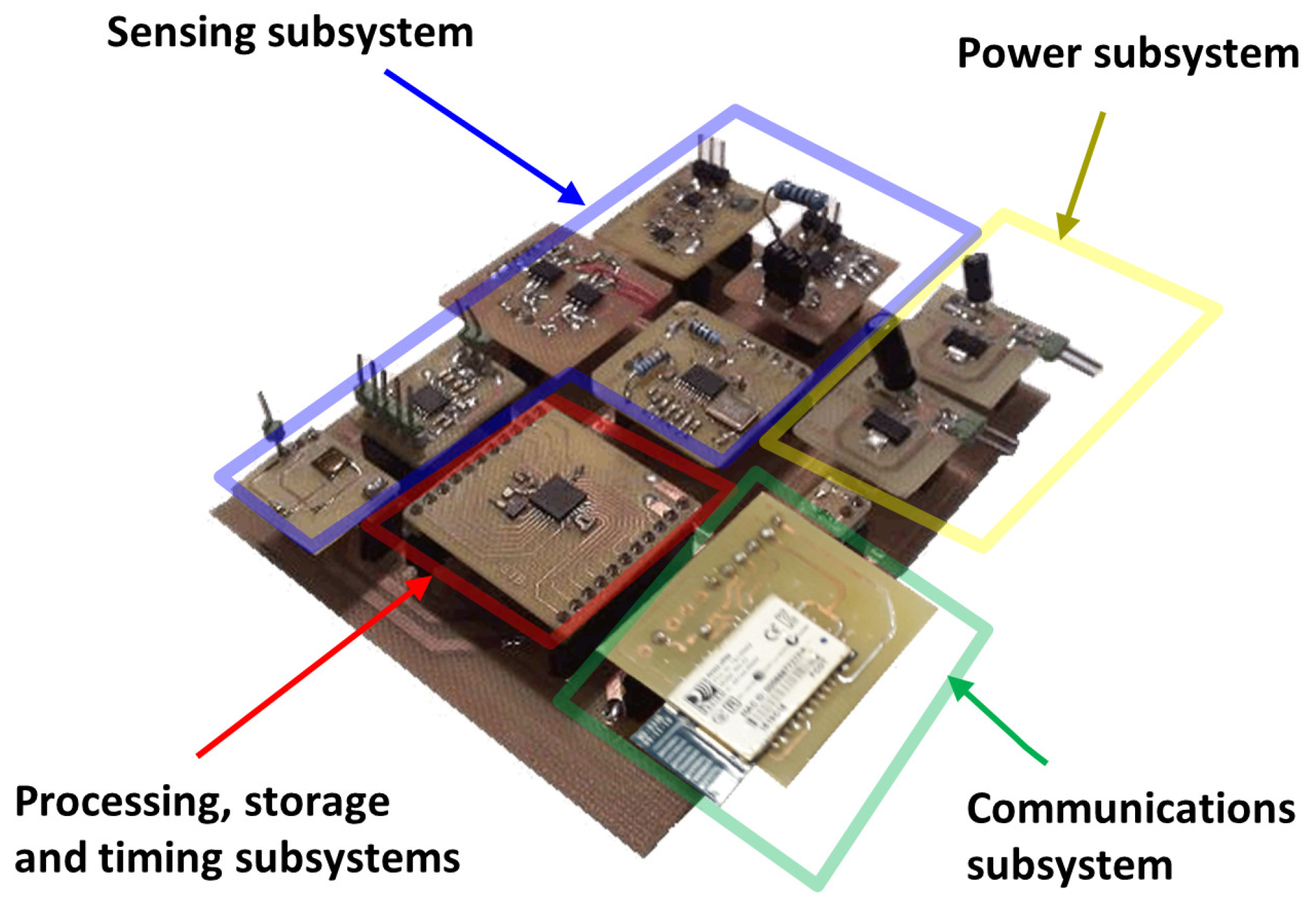
2.2. Architecture of the Smart Bioimpedance Device
- Sensing subsystem: Which encompasses the necessary hardware to perform bioimpedance measurements. The referred subsystem generates an alternating electric current of known amplitude to be injected into the human body through two electrodes (distal electrodes). By means of two other electrodes located in the current path (proximal electrodes) the sensing subsystem makes a measurement of the voltage generated by the circulation of the current. Two 150-cm cables connect the smart bioimpedance device with the electrodes: a cable for the electrodes to be placed on the hand and another one for the electrodes to be placed on the foot. Each cable has two lines, and each line is shielded to reduce the effects of electromagnetic noise. The cables end in crocodile clips for the connection with the electrodes.
- Processing subsystem: Integrates the hardware, software and firmware elements of the smart bioimpedance device that are applied in the processing for the estimations of the module and phase of bioimpedance in each of the frequencies. Frequencies can be configured remotely by sending a command. The processing subsystem is also responsible for the correct activation and configuration of the different modules of the sensing subsystem each time a new bioimpedance measurement is performed. Thus, the energy consumption of the smart bioimpedance device is reduced, deriving the different modules from the sensing subsystem to low consumption modes of operation when they are not necessary. The processing subsystem is implemented in a microprocessor with an 8-bit arithmetic-logic unit that operates at 4 MHz (PIC18LF2431 microprocessor from Microchip). Pre-processing algorithms are programmed in the microprocessor’s flash memory, which has a capacity of 16 Mbytes.
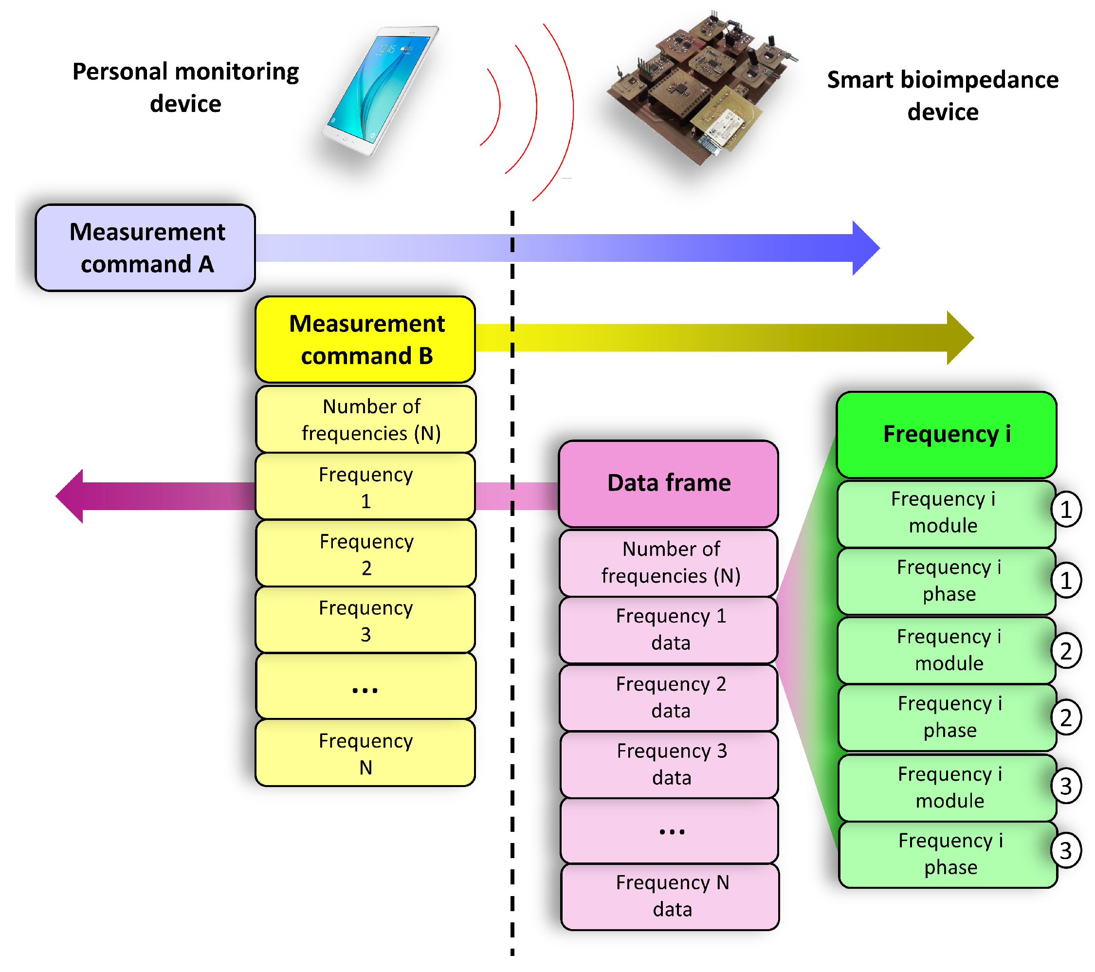
- Communications subsystem: RN42 module from Microchip has been used for the development of the wireless communications of the smart bioimpedance device according to the SPP profile of Bluetooth v2.1 standard. Communications are bidirectional to allow the sending of results of the processing subsystem in one way, and the remote configuration of the smart sensor by sending commands in the other way. According to the communications protocol for the device control, the personal monitoring device starts a bioimpedance measurement by sending a command (Measurement command A in Figure 2). The frequencies are pre-configured in the smart bioimpedance device, although it is also possible to define the number and value of the frequencies to be acquired by sending a special command (Measurement command B). Once the multifrequency measurement is finished, the smart bioimpedance device sends a response data frame containing the frequencies (Data frame), the modulus and phase of the bioimpedance following the data structure described in Figure 2. It should be mentioned that for each frequency, three consecutive estimations of the bioimpedance modulus and phase are performed, which are also sent in the data frame to provide a more robust measurement. Depending on the dispersion of bioimpedance values, the personal monitoring device may decide to use the average value of the three measurements or discard the frequency in the identification of parameters of a three-dispersion bioimpedance model.
- Data storage subsystem: It is responsible for the correct storage of the data used by the smart bioimpedance device. To develop the data storage subsystem, the 768-byte SRAM memory and the 256-byte EEPROM memory of the PIC18LF2431 microprocessor are used.
- Timing subsystem: Which deals with the maintenance of a real-time timing system and the assignment to each measurement of the time in which they were made for registration and subsequent monitoring. Such subsystem is also responsible for notifying the processing subsystem of the instants for carrying out operations whose timing has been pre-configured. An external crystal of 32.768 kHz and one of the microprocessor timers are used to manage its operation. The timing subsystem is also implemented in the program code of PIC18LF2431 microprocessor by managing the interrupts of one of the microprocessor’s internal timers. An external crystal clock of 32.768 KHz is used to precisely define the timing with a real-time clock.
- Energy subsystem: Provides the necessary supply voltages for the proper operation of all subsystems. A lithium polymer battery with 3.7 nominal voltage provides power for device operation. BQ21040 charger device from Texas Instruments is used to manage the battery charge. A LD1117S33TR regulator from STMicroelectronics provides 3.3 V supply voltage for the digital electronic components (microprocessor, transceiver, etc.). The TPS65133 DC-DC converter from Texas Instruments is employed to supply the ±5.0 V required for the sensing subsystem. The microprocessor can turn off the analog electronics of the sensing subsystem through a line that controls the operation of TPS65133 component, in order to reduce energy consumption.
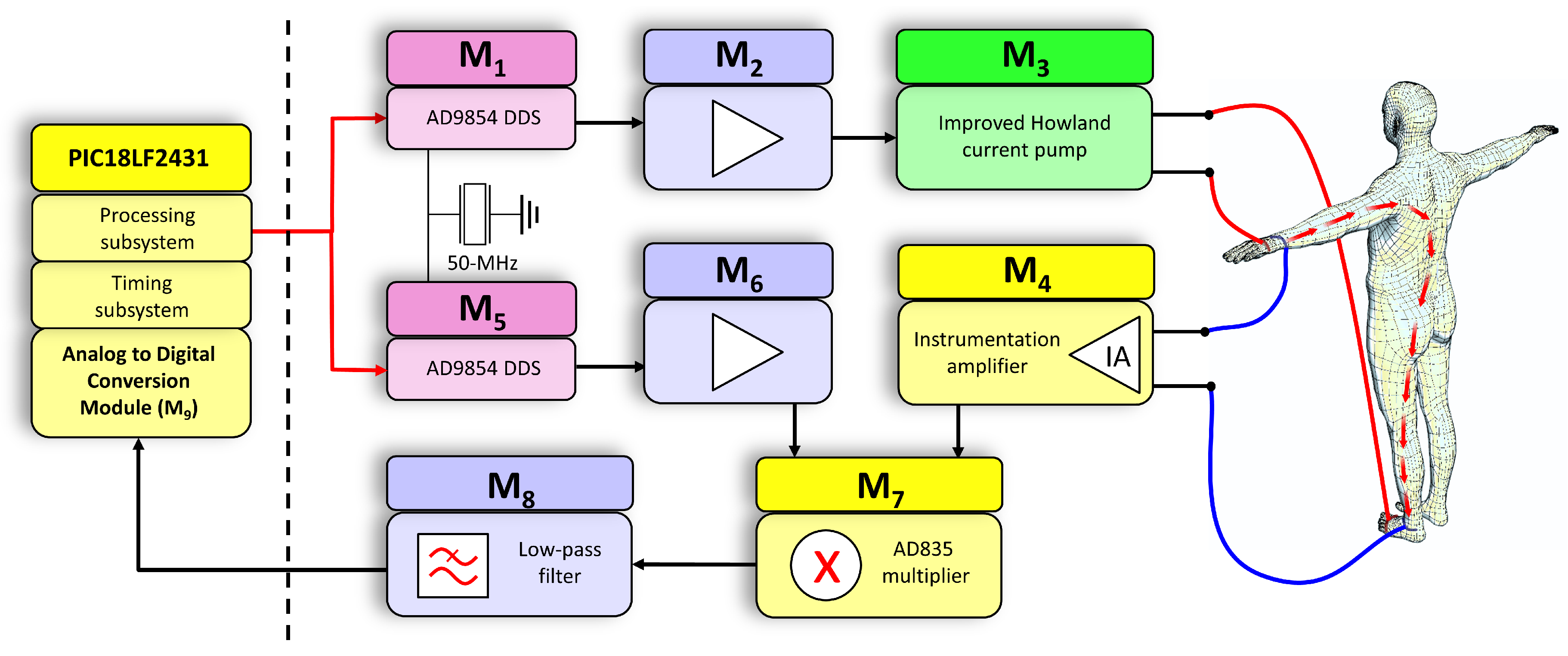
2.3. Architecture of the Sensing Subsystem
- Injection signal generation module (): This is a programmable oscillator that uses the Direct Digital Frequency Synthesis (DDS) technique. This module generates a sine voltage waveform () with fixed amplitude (). The frequency () of the signal () can be configured to scan bioimpedance measurements at different configurable frequencies. AD9854 high-speed DDS from Analog Devices has been used to generate a high-precision sine waveform capable of being configured to generate any frequency from 0.19 Hz to 5 MHz, with a resolution of 0.19 Hz and a stability of 40 ppm. A 50-MHz clock was used to provide the necessary synchronization for the operation of the DDS. The PIC18LF2431 microprocessor controls the frequency and phase of the signal generated by the DDS through a serial data interface. This scheme gives the system great flexibility to generate signals of different frequency. As mentioned previously, the frequencies of this sweep can be configured remotely by means of a command so that they usually take any value between 1 kHz and 1 MHz in a body bioimpedance measurement application (lower frequencies are not recommended to avoid interfering with the biological signals and higher frequencies are more sensitive to electromagnetic noise [1]) although depending on the application this range can be extended to both low and high frequencies (from 0.19 Hz to 5 MHz). As also mentioned, the number of frequencies of the bioimpedance measurement scan is also a configurable parameter, although a single-frequency analysis can be performed as well. An input line to the DDS, also controlled by the microprocessor, allows it to be configured in a low-energy mode, in which the operation of the device is suspended and the signal generation process is canceled. Signal discontinuities due to digital sampling are smoothed through an low-pass filter inside the DDS with a cutoff frequency high enough not to affect the generated signals.
- Injection signal amplification module (): Amplifier with () gain applied on signal () to generate signal (). Since the output signal of the DDS is very weak (about 0.6 Vpp), an amplifier based on operational amplifiers (OpAmps) is used to increase the signal amplitude. This module also has the function of decoupling the DDS from the voltage-current conversion module (the DDS has an output resistance of 50 ), providing a suitable voltage level for its operation.
- Voltage-current conversion module (): Transconductance amplifier that converts the voltage signal at the output of the injection signal amplification module () into a current signal (), injected into the human body through the distal electrodes. The amplitude () of the injected current intensity has a constant value, preset to comply with international safety standards [1]. In addition, the referred current amplitude is independent of the impedance of the human body, the impedance of the electrodes and the frequency at which the measurement is made. An improved Howland current pump [34,35] has been used for its implementation, due to its precision and stability characteristics, through OpAmps. The current source was configured to generate an effective current of 0.4 mA, well below the international safety limits for this type of applications [36].
- Signal detection module (): Instrumentation amplifier that applies a gain () to the voltage detected through the proximal electrodes (), generating the signal (). The input impedance of the instrumentation amplifier is very high so that the voltage drop in the proximal electrodes can be considered negligible. The instrumentation amplifier has been implemented through discrete low-noise OpAmps, providing a gain of 2, a bandwidth of 45 MHz, a common-mode rejection ratio (CMRR) of 94 dB and an input impedance of 1 .
- Internal signal generation module (): It generates an internal sine voltage waveform () with the same amplitude value () and frequency () as the signal (), but with a phase difference () that alternates its values between 0 and 90 to measure the in-phase and quadrature components. Another DDS with the same characteristics as () is used for its implementation. This is a relevant aspect of the present design, which allows precise control of the phase measurement and, together with the possibility of controlling the measurement frequency, allows the device to be used for different applications. This phase and frequency control is the basis of the calibration procedure described in Section 2.4. In addition, the proposed scheme allows the use of only a single multiplier to perform the demodulation of signals in phase and quadrature, which is the principle used for the measurement of the biompedance modulus and phase [1,37]. The measurement process is carried out in two stages: first, a frequency sweep in which the parameter takes the value 0 is carried out for the evaluation of in-phase components; second, a subsequent frequency sweep with set to 90 is performed to measure the quadrature-phase components. The processing subsystem is responsible for configuring this transition in the phase, waiting for the required time for the signals to stabilize before the measurement is performed. The use of two DDS caused a continuous drift of the phase lag between the signals generated by both DDS over time (the phase lag did not remain fixed, but increased or decreased over time), making difficult the phase control between the signals generated by both DDS. This effect was more evident the higher the frequency. The cause of the drift in the phase came from the difference in the frequency of the crystal clocks that controlled each DDS, however small this difference was. This problem was solved by employing a single 50-MHz crystal used as time reference for both DDS. Thus, both devices have exactly the same frequency and the offset between the signals of both modules remains constant over time.
- Internal signal amplification module (): Amplifier with () gain applied on signal () to generate signal (). The function of this module is to decouple the module () from the module (), also adapting the voltage of the sine waveform to adequate levels of operation. It has been implemented using discrete OpAmps.
- Multiplier module (): This module generates signal () as a result of the multiplication of signal () and signal (). A AD835 full complete four-quadrant multiplier from Analog Devices has been used for this purpose. The resulting signal () is formed by the superposition of a sinusoidal waveform with frequently () and a continuous level that depends on the phase lag between the input signals and their amplitudes. Thus, the continuous level of in-phase and quadrature components allow to calculate the bioimpedance modulus and phase by means of a coherent demodulation process [1,37].
- Filtering module (): It is an active second-order low pass filter based on OpAmps with a cut-off frequency of 13.8 Hz that extracts the continuous component () from signal (). The filter cutoff frequency is low enough to keep the signal ripple below 1% with respect to the continuous level at all operating frequencies.
- Analog to Digital Conversion Module (): This module is responsible for converting the analog signal () into digital signals with which the processing subsystem can operate. It is responsible for calculating the bioimpedance modulus and phase following the standard procedure of demodulation of signals in quadrature [1], taking into account the characteristics of the proposed scheme. For its implementation, one of the 10-bit analog-digital converters of the microprocessor has been used, setting the maximum voltage to provide a resolution of 1.17 mV.
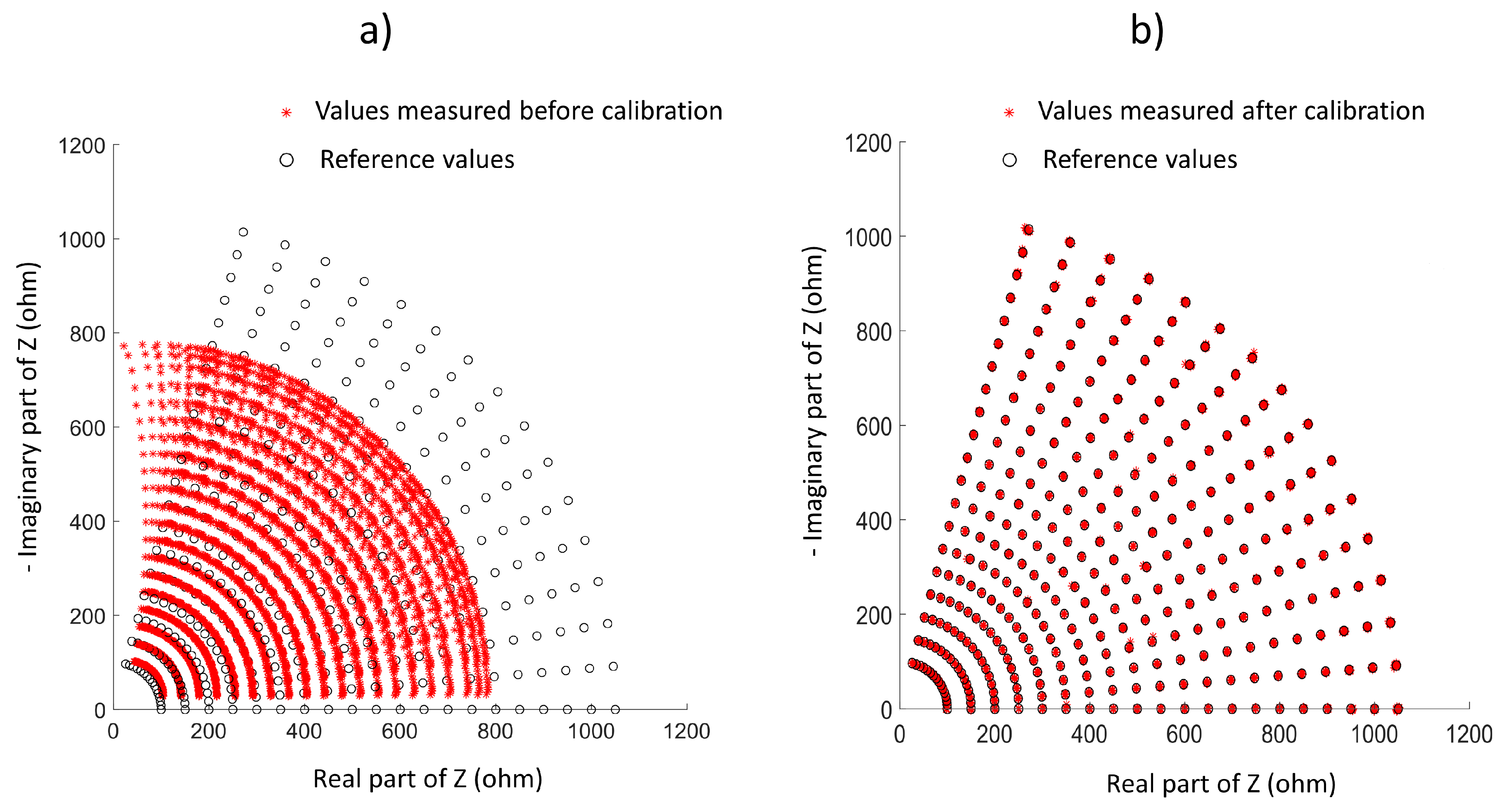
2.4. Addressing Parasitic Effects
- For the calibration of the device a series resistor pattern set was used, which allowed testing values in the range from 100 up to 1050 with increments of 50 .
- The device was configured to evaluate sequentially 16 phase values, modeling the phase shift between the output signal and the internal reference signal. This way, phase could be swept in increments of 5 from 0 to 75.
- For each resistor value of the calibration pattern and each evaluated phase, an automatic full frequency sweep was performed, and changing the resistance value after all phases were evaluated.
- The full process was repeated 5 times to provide a better robustness against measurement noise.
- The measured values were compared against the reference values to provide a fitting of the calibration curves in terms of frequency, impedance modulus and phase.
2.5. Proposed Artefact-Aware Bioimpedance Model
2.6. Description of the Proposed Algorithm
- It is an algorithm able to identify the parameters of a Cole model of three dispersions. To the authors’ knowledge, no procedure or algorithm has been published that explicitly solves the parameter identification in a three-dispersion bioimpedance model. In addition, and as detailed in Section 2.5, the first and third dispersion of the proposed model are not related to bioimpedance values, but to artefacts that may appear at low and high frequencies, and if they are not removed or taken into account, can greatly affect in the parameters identification process.
- It is a low-computational-load algorithm capable of being efficiently solved in a low-performance microprocessor thanks to a novel approach that analytically solves the model on an iterative scan in a single parameter ().
- Load N complex measured impedance values (real and imaginary parts), in N consecutive frequencies.
- The base of the processing is an iterative search of the solution for a single parameter of the model, the parameter (from to in increments of ). The main advantage of this approach is that the search of the solution depends only on one parameter, such that the required number of iterations is appreciably reduced.
- For each value of , the bioimpedance values are corrected according to the expression of , where index i refers to the frequency. is the impedance that would be obtained if the influence of the delay modeled by were removed.
- The impedance values are grouped into sectors, which might overlap. The algorithm will cover the different bioimpedance sectors to find the best fit with the second dispersion, where s indicates the number of the sector.
- Identification of the Cole model (second dispersion) that best fits the impedances of sector s.
- If s is higher than 1, identification of the Cole model (first dispersion) that best fits the result of subtracting the second dispersion to the corrected impedances , considering only the lower frequencies.
- If s is lower than , identification of the Cole model (third dispersion) that best fits the result of subtracting the second dispersion to the corrected impedances , considering only the higher frequencies.
- Calculation of the mean square error (MSE) between the measured impedance values and those obtained from the three-dispersion model. If this error is the smaller until then, the parameters evaluated are proposed as the actual solution of the model. Finally, the algorithm loop is closed with the execution of step 2.
- 9.
- The impedance values analyzed are grouped in sets of three elements in each iteration: one corresponding to a low frequency (index ), another to a medium frequency (index ) and the last one to a high frequency (index ). Index values are pre-configured to sweep all frequencies in a pseudo-random way, avoiding the repetition of triplets.
- 10.
- If the real and the imaginary parts of the absolute value of the bioimpedance are plotted for each of the sets, three points are obtained in the first quadrant. When three points are defined in a plane, it is possible to define a fourth point which is equidistantly located with respect to the other three. This property is used to calculate the radius and the point corresponding to the center of the circle that matches the three points, taking into account that the center corresponds to the fourth point and the radius with the distance mentioned.
- 11.
- The values of the parameters , and for each of the sets of three impedances are calculated from the angle between the real axis, the cut-off point of the circumference closest to the origin, and the center of the semicircle.
- 12.
- Once the impedance semicircle is defined, each of the impedances of the triplet define a time constant according to the model described in (1). The proposed time constant will be the arithmetic mean of the three time constants. The time constant value can be solved from the real part of the expression (1).
- 13.
- Calculation of the MSE between the impedance values and those obtained from the model. If this error is the smaller until then, the parameters evaluated are proposed as the local solution of the model for the dispersion evaluated. Finally, the procedure loop is closed with the execution of step 9.
2.7. Description of the Hardware Validation Study
2.8. Description of the Software Validation Study
- Mean relative error ().
- Maximum relative error ().
- Standard deviation of the relative error ().
- : Nonlinear Least Squares of the bioimpedance modulus [25].
- : Least Squares fitting of the admittance with correction of the parasitic capacitance [32].
- : Curve fitting based on Least Squares method [27].
- : Curve fitting based on Least Absolute Deviation method [27].
- : Bacterial foraging optimization algorithm [30].
- : Algorithm implemented in the Body Composition Monitor (BCM) of Fresenius Medical Care.
3. Results
3.1. Results of the Hardware Validation Study
3.2. Results of the Software Validation Study
- Example A: In the majority of the cases studied, no parasitic effect was observed in the bioimpedance measurements at high or low frequency, which could be verified by analyzing the results of the proposed algorithm. As an example, Figure 9 shows the conventional cole diagram of a bioimpedance measurement performed on a voluntary. In this case, both the BCM extended Cole model and the proposed algorithm agreed in the process of identifying the bioimpedance model. and were very close (, , , ), and therefore, the estimation of body composition.
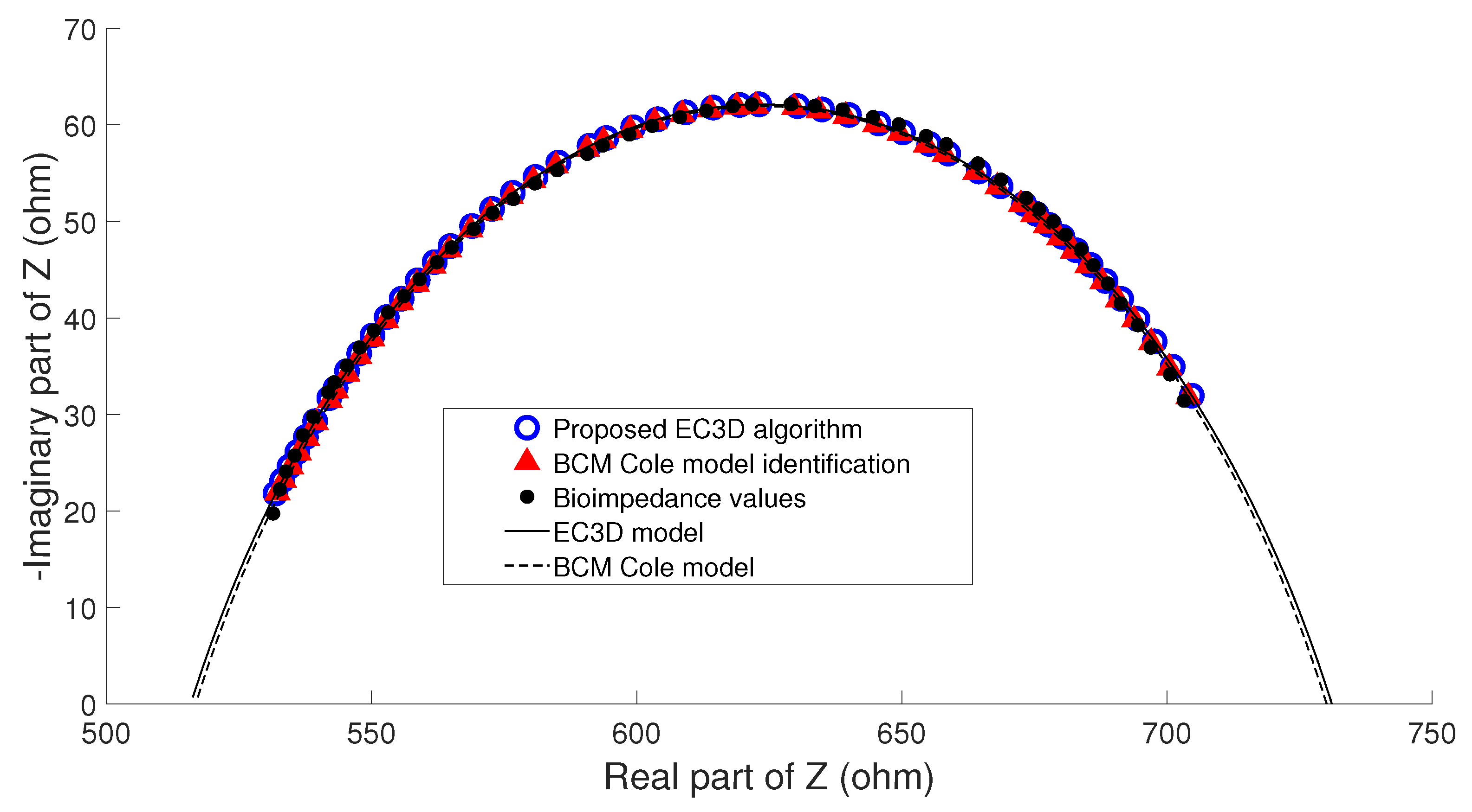
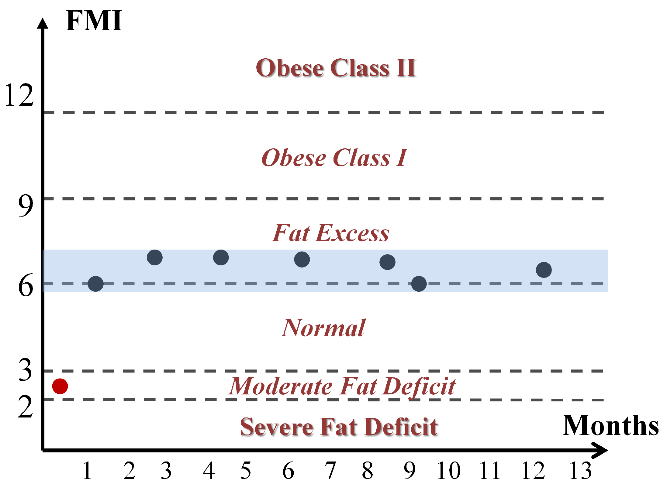
- Example B: Figure 10 shows bioimpedance values of a patient measurement on a Cole diagram. Bioimpedance values show a hook up effect at high frequency. As mentioned in Section 2.4, a possible cause of this behavior may be the parasitic capacitance established between the human body and the ground plane [63]. This effect was corrected by the BCM extended Cole model incorporating a major phase delay ( nseg). However, it can be observed that bioimpedance values do not fit the model at both high and intermediate frequencies. On the other hand, the proposed algorithm matched this disturbance effect at high frequency with an additional dispersion, obtaining a better fit to the bioimpedance values. The result was a discrepancy in the identification of the parameters of the bioimpedance model (, , , ), which also resulted in differences in the estimation of body composition.The evolution of the nutritional status of the patient in example B according to the percentage of fat is shown in Figure 11, which was assessed by means of bioimpedance measurements. The dots in the figure indicate the value of the percentage of fat in the time instants in which the measurements were made. Dashed lines allow to visually classify the state of the patient according to [75]. The dot with different color (measurement 4) shows a significant variation in the nutritional status with respect to the other estimations, which are grouped on the colored band.
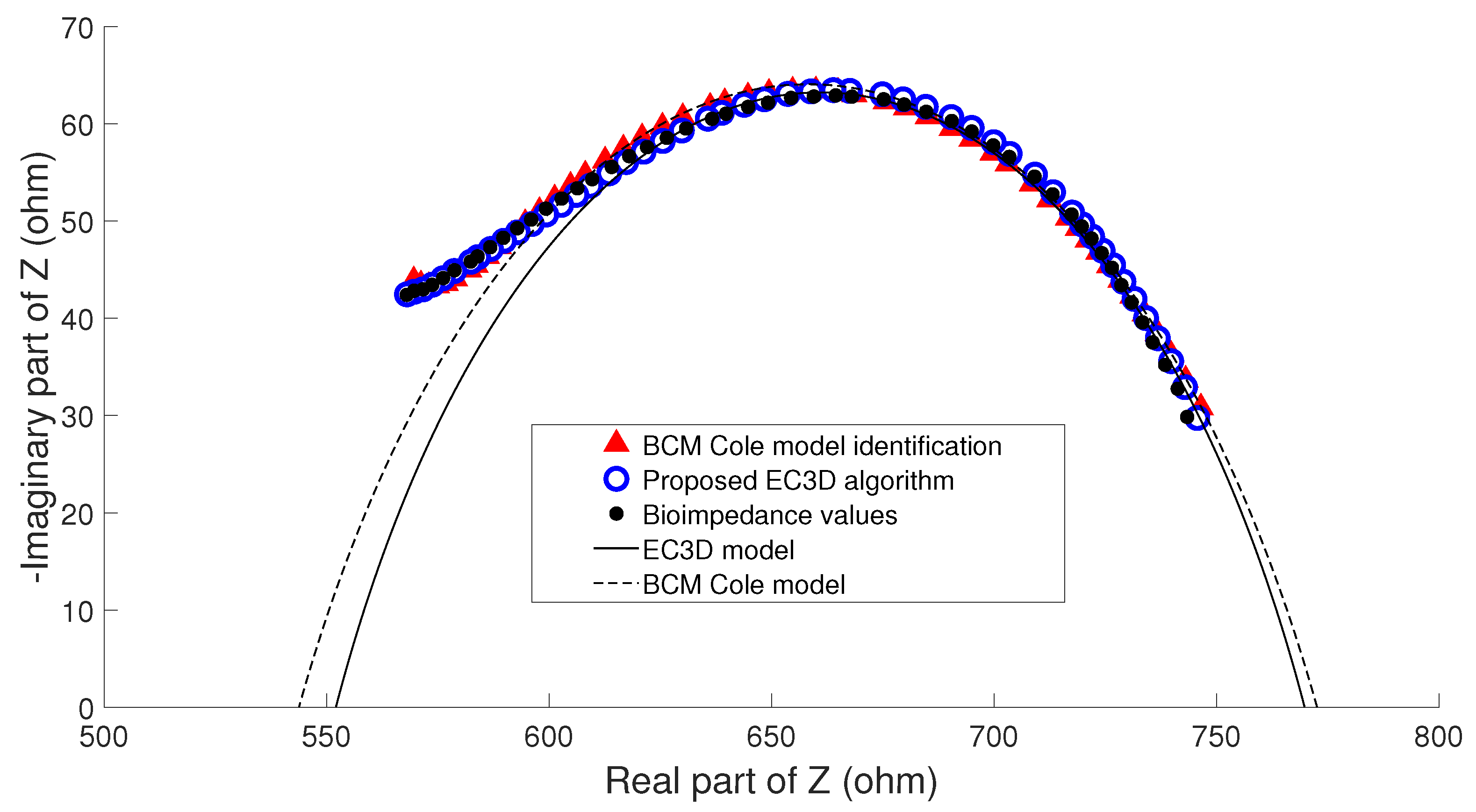
- Example C: Figure 12 also shows bioimpedance values of another patient measurement. In this other case, a hook up effect appears at low frequency. Although this type of bioimpedance behavior moves away from the expected response of a body bioimpedance measurement, as was mentioned in Section 2.4, this type of phenomenon can occur when there is a bad contact between the electrode and the skin, which results in a high value of the electrode impedance [58,59,61,62]. Our experiences corroborate this fact, since when during the experiments on patients hook up effects were observed at low frequency, it was found that in many cases one of the electrodes was not well attached to the skin. The replacement of the electrode and the repetition of the measurement solved the problem. Even so, some of the cases were not detected at the time of the measurement (one of them is Example C), which indicates the need to incorporate a method of detection of such artefacts in the measurement equipment and/or a procedure to correct them. In this case, the BCM model tried to approximate the bioimpedance values by a large phase lead ( nseg), but a relevant mismatch is observed in all the frequency range. The proposed algorithm corrected this disturbance effect with an additional dispersion at low frequency, also getting a good fit to the bioimpedance values. In this case, a large difference was found in the value of identified by each model (, , , ), giving rise to differences also in body composition.
4. Conclusions
Author Contributions
Funding
Acknowledgments
Conflicts of Interest
Abbreviations
| BC | Body Composition |
| BCM | Body Composition Monitor |
| BCMa | BCM device algorithm |
| BFO | Bacterial foraging optimization algorithm |
| CMRR | Common-Mode Rejection Ratio |
| COPD | Chronic Obstructive Pulmonary Disease |
| DDS | Direct Digital Frequency Synthesis |
| EC3D | Extended Cole model with 3 Dispersions algorithm |
| ECW | Extracellular Water |
| FFM | Fat Free Mass |
| FM | Fat Mass |
| GA | Genetic algorithm |
| HD | Hemodialysis |
| ICW | Intracellular Water |
| LAD | Curve fitting based on Least Absolute Deviation method |
| LS | Curve fitting based on Least Squares method |
| LSC | Least Squares fitting of the admittance with correction of the parasitic capacitance |
| LSM | Nonlinear Least Squares of the bioimpedance modulus |
| MaxRE | Maximum relative error |
| MeanRE | Mean relative error |
| MSE | Mean square error |
| NLLS | Nonlinear Least Squares |
| OpAmps | Operational amplifiers |
| PD | Peritoneal Dialysis |
| PSO | Particle-swarm optimization algorithm |
| SDRE | Standard deviation of the relative error |
| TBW | Total Body Water |
References
- Naranjo-Hernández, D.; Reina-Tosina, J.; Min, M. Fundamentals, recent advances, and future challenges in bioimpedance devices for healthcare applications. J. Sens. 2019, 2019. [Google Scholar] [CrossRef] [Green Version]
- Roa, L.M.; Naranjo, D.; Reina-Tosina, J.; Lara, A.; Milán, J.A.; Estudillo, M.A.; Oliva, J.S. Applications of bioimpedance to end stage renal disease (ESRD). Stud. Comput. Intell. 2013, 404, 689–769. [Google Scholar]
- Moissl, U.; Wabel, P.; Chamney, P.; Bosaeus, I.; Levin, N.W.; Bosy-Westphal, A.; Korth, O.; Müller, M.J.; Ellegård, L.; Malmros, V.; et al. Body fluid volume determination via body composition spectroscopy in health and disease. Physiol. Meas. 2006, 27, 921–933. [Google Scholar] [CrossRef]
- Ellegard, L.; Aldenbratt, A.; Svensson, M.; Lindberg, C. Body composition in patients with primary neuromuscular disease assessed by dual energy X-ray absorptiometry (DXA) and three different bioimpedance devices. Clin. Nutr. ESPEN 2019, 29, 142–148. [Google Scholar] [CrossRef]
- Peppa, M.; Stefanaki, C.; Papaefstathiou, A.; Boschiero, D.; Dimitriadis, G.; Chrousos, G. Bioimpedance analysis vs. DEXA as a screening tool for osteosarcopenia in lean, overweight and obese caucasian postmenopausal females. Hormones 2017, 16, 181–193. [Google Scholar]
- Piuri, G.; Ferrazzi, E.; Bulfoni, C.; Mastricci, L.; Di Martino, D.; Speciani, A. Longitudinal changes and correlations of bioimpedance and anthropometric measurements in pregnancy: Simple possible bed-side tools to assess pregnancy evolution. J. Mater.-Fetal Neonatal Med. 2017, 30, 2824–2830. [Google Scholar] [CrossRef] [PubMed]
- Zajac-Gawlak, I.; Klapcinska, B.; Kroemeke, A.; Pospiech, D.; Pelclova, J.; Pridalova, M. Associations of visceral fat area and physical activity levels with the risk of metabolic syndrome in postmenopausal women. Biogerontology 2017, 18, 357–366. [Google Scholar] [CrossRef] [PubMed] [Green Version]
- Siriopol, D.; Onofriescu, M.; Voroneanu, L.; Apetrii, M.; Nistor, I.; Hogas, S.; Kanbay, M.; Sascau, R.; Scripcariu, D.; Covic, A. Dry weight assessment by combined ultrasound and bioimpedance monitoring in low cardiovascular risk hemodialysis patients: A randomized controlled trial. Int. Urol. Nephrol. 2017, 49, 143–153. [Google Scholar] [CrossRef] [PubMed]
- Kim, E.J.; Choi, M.J.; Lee, J.H.; Oh, J.E.; Seo, J.W.; Lee, Y.K.; Yoon, J.W.; Kim, H.J.; Noh, J.W.; Koo, J.R. Extracellular fluid/intracellular fluid volume ratio as a novel risk indicator for all-cause mortality and cardiovascular disease in hemodialysis patients. PLoS ONE 2017, 12, e0170272. [Google Scholar] [CrossRef] [Green Version]
- Demirci, C.; Aşcı, G.; Demirci, M.S.; Özkahya, M.; Töz, H.; Duman, S.; Sipahi, S.; Erten, S.; Tanrısev, M.; Ok, E. Impedance ratio: A novel marker and a powerful predictor of mortality in hemodialysis patients. Int. Urol. Nephrol. 2016, 48, 1155–1162. [Google Scholar] [CrossRef]
- Shah, C.; Vicini, F.; Arthur, D. Bioimpedance Spectroscopy for Breast Cancer Related Lymphedema Assessment: Clinical Practice Guidelines. Breast J. 2016, 22, 645–650. [Google Scholar] [CrossRef] [PubMed]
- Redondo-del Río, M.; Camina-Martín, M.; Moya-Gago, L.; de-la Cruz-Marcos, S.; Malafarina, V.; de Mateo-Silleras, B. Vector bioimpedance detects situations of malnutrition not identified by the indicators commonly used in geriatric nutritional assessment: A pilot study. Exp. Gerontol. 2016, 85, 108–111. [Google Scholar] [CrossRef] [PubMed]
- Shin, H.; Kim, D.K.; Seo, K.; Kang, S.; Lee, S.; Son, S. Relation between respiratory muscle strength and skeletal muscle mass and hand grip strength in the healthy elderly. Ann. Rehabil. Med. 2017, 41, 686–692. [Google Scholar] [CrossRef] [PubMed]
- Dégi, A.; Bárczi, A.; Szabó, D.; Éva, E.; Reusz, G.; Dezsfi, A. Cardiovascular risk assessment in pediatric liver transplant patients. J. Pediatr. Gastroenterol. Nutr. 2019, 68, 377–383. [Google Scholar] [CrossRef] [PubMed]
- Lyons, K.; Bischoff, M.; Fonarow, G.; Horwich, T. Noninvasive bioelectrical impedance for predicting clinical outcomes in outpatients with heart failure. Crit. Pathw. Cardiol. 2017, 16, 32–36. [Google Scholar] [CrossRef]
- Lee, J.; Ryu, H.; Yoon, S.; Kim, E.; Yoon, S. Extracellular-to-Intracellular Fluid Volume Ratio as a Prognostic Factor for Survival in Patients With Metastatic Cancer. Integr. Cancer Ther. 2019, 18. [Google Scholar] [CrossRef] [Green Version]
- Tinsley, G.; Graybeal, A.; Moore, M.; Nickerson, B. Fat-free Mass Characteristics of Muscular Physique Athletes. Med. Sci. Sports Exer. 2019, 51, 193–201. [Google Scholar] [CrossRef]
- Rossi, S.; Mancarella, C.; Mocenni, C.; Della Torre, L. Bioimpedance sensing in wearable systems: From hardware integration to model development. In Proceedings of the RTSI 2017—IEEE 3rd International Forum on Research and Technologies for Society and Industry, Modena, Italy, 11–13 September 2017. [Google Scholar]
- De Carvalho, P.; Palacio, J.; Van Noije, W. Area optimized CORDIC-based numerically controlled oscillator for electrical bio-impedance spectroscopy. In Proceedings of the 2016 IEEE International Frequency Control Symposium, New Orleans, LA, USA, 9–12 May 2016. [Google Scholar]
- Ismail, A.; Leonhardt, S. Simulating non-specific influences of body posture and temperature on thigh-bioimpedance spectroscopy during continuous monitoring applications. In Journal of Physics: Conference Series; IOP Publishing: Bristol, UK, 2013; Volume 434. [Google Scholar]
- Maundy, B.; Elwakil, A. Extracting single dispersion Cole-Cole impedance model parameters using an integrator setup. Analog Integr. Circuits Signal Process. 2012, 71, 107–110. [Google Scholar] [CrossRef]
- Freeborn, T.; Maundy, B.; Elwakil, A. Least squares estimation technique of Cole-Cole parameters from step response. Electron. Lett. 2012, 48, 752–754. [Google Scholar] [CrossRef]
- Freeborn, T.; Maundy, B.; Elwakil, A. Improved Cole-Cole parameter extraction from frequency response using least squares fitting. In Proceedings of the ISCAS 2012—2012 IEEE International Symposium on Circuits and Systems, Seoul, Korea, 20–23 May 2012; pp. 337–340. [Google Scholar]
- Ward, L.; Essex, T.; Cornish, B. Determination of Cole parameters in multiple frequency bioelectrical impedance analysis using only the measurement of impedances. Physiol. Meas. 2006, 27, 839–850. [Google Scholar] [CrossRef]
- Buendia, R.; Gil-Pita, R.; Seoane, F. Cole parameter estimation from total right side electrical bioimpedance spectroscopy measurements Influence of the number of frequencies and the upper limit. In Proceedings of the Annual International Conference of the IEEE Engineering in Medicine and Biology Society, EMBS, Boston, MA, USA, 30 August–3 September 2011; pp. 1843–1846. [Google Scholar]
- Nordbotten, B.; Tronstad, C.; Martinsen, Ø.G.; Grimnes, S. Evaluation of algorithms for calculating bioimpedance phase angle values from measured whole-body impedance modulus. Physiol. Meas. 2011, 32, 755–765. [Google Scholar] [CrossRef] [Green Version]
- Yang, Y.; Ni, W.; Sun, Q.; Wen, H.; Teng, Z. Improved Cole parameter extraction based on the least absolute deviation method. Physiol. Meas. 2013, 34, 1239–1252. [Google Scholar] [CrossRef] [PubMed]
- Sasaki, K.; Wake, K.; Watanabe, S. A dosimetric study using best-fit Cole-Cole parameters of biological tissues and organs in radio frequency band. In Proceedings of the 2013 International Symposium on Electromagnetic Theory, Hiroshima, Japan, 20–24 May 2013; pp. 630–633. [Google Scholar]
- Paterno, A.; Hermann Negri, L.; Bertemes-Filho, P. Efficient Computational Techniques in Bioimpedance Spectroscopy. In Applied Biological Engineering—Principles and Practice; Naik, G.R., Ed.; InTech: Vienna, Austria, 2012; Chapter 1; pp. 3–28. [Google Scholar]
- Gholami-Boroujeny, S.; Bolic, M. Extraction of Cole parameters from the electrical bioimpedance spectrum using stochastic optimization algorithms. Med. Biol. Eng. Comput. 2016, 54, 643–651. [Google Scholar] [CrossRef] [PubMed]
- Halter, R.; Hartov, A.; Paulsen, K.; Schned, A.; Heaney, J. Genetic and least squares algorithms for estimating spectral EIS parameters of prostatic tissues. Physiol. Meas. 2008, 29, S111–S123. [Google Scholar] [CrossRef] [PubMed]
- Wu, H.; Zuo, Y.; Wei, F.; Zhao, N.; Wu, H.; Song, H.; Gu, S.; Wang, X.; Zhang, J. Study on complex Td correction and Cole-Cole parameters for the impedance of immunobiosensor. In Proceedings of the ICAE 2011 Proceedings: 2011 International Conference on New Technology of Agricultural Engineering, Zibo, China, 27–29 May 2011; pp. 806–809. [Google Scholar]
- Kassanos, P.; Constantinou, L.; Triantis, I.; Demosthenous, A. An integrated analog readout for multi-frequency bioimpedance measurements. IEEE Sens. J. 2014, 14, 2792–2800. [Google Scholar] [CrossRef]
- Tucker, A.S.; Fox, R.M.; Sadleir, R.J. Biocompatible, High Precision, Wideband, Improved Howland Current Source With Lead-Lag Compensation. IEEE Trans. Biomed. Circuits Syst. 2013, 7, 63–70. [Google Scholar] [CrossRef] [PubMed]
- Sanders, J.E.; Moehring, M.A.; Rothlisberger, T.M.; Phillips, R.H.; Hartley, T.; Dietrich, C.R.; Redd, C.B.; Gardner, D.W.; Cagle, J.C. A Bioimpedance Analysis Platform for Amputee Residual Limb Assessment. IEEE Trans. Biomed. Eng. 2016, 63, 1760–1770. [Google Scholar] [CrossRef] [Green Version]
- Ferreira, J.; Pau, I.; Lindecrantz, K.; Seoane, F. A Handheld and Textile-Enabled Bioimpedance System for Ubiquitous Body Composition Analysis. An Initial Functional Validation. IEEE J. Biomed. Health Inform. 2017, 21, 1224–1232. [Google Scholar] [CrossRef]
- Hersek, S.; Töreyin, H.; Teague, C.N.; Millard-Stafford, M.L.; Jeong, H.K.; Bavare, M.M.; Wolkoff, P.; Sawka, M.N.; Inan, O.T. Wearable Vector Electrical Bioimpedance System to Assess Knee Joint Health. IEEE Trans. Biomed. Eng. 2017, 64, 2353–2360. [Google Scholar] [CrossRef]
- Bartels, E.; Sørensen, E.; Harrison, A. Multi-frequency bioimpedance in human muscle assessment. Physiol. Rep. 2015, 3, e12354. [Google Scholar] [CrossRef]
- Fernandez, R.E.; Lebiga, E.; Koklu, A.; Sabuncu, A.C.; Beskok, A. Flexible Bioimpedance Sensor for Label-Free Detection of Cell Viability and Biomass. IEEE Trans. Nanobiosci. 2015, 14, 700–706. [Google Scholar] [CrossRef] [PubMed]
- Callejón, M.A.; del Campo, P.; Reina-Tosina, J.; Roa, L.M. A Parametric Computational Analysis into Galvanic Coupling Intrabody Communication. IEEE J. Biomed. Health Inform. 2018, 22, 1087–1096. [Google Scholar] [CrossRef] [PubMed]
- Taji, B.; Shirmohammadi, S.; Groza, V.; Batkin, I. Impact of Skin-Electrode Interface on Electrocardiogram Measurements Using Conductive Textile Electrodes. IEEE Trans. Instrum. Meas. 2014, 63, 1412–1422. [Google Scholar] [CrossRef]
- McEwan, A.; Cusick, G.; Holder, D. A review of errors in multi-frequency EIT instrumentation. Physiol. Meas. 2007, 28, S197–S215. [Google Scholar] [CrossRef]
- Yu, K.; Shao, Q.; Ashkenazi, S.; Bischof, J.C.; He, B. In Vivo Electrical Conductivity Contrast Imaging in a Mouse Model of Cancer Using High-Frequency Magnetoacoustic Tomography With Magnetic Induction (hfMAT-MI). IEEE Trans. Med. Imaging 2016, 35, 2301–2311. [Google Scholar] [CrossRef]
- Kubendran, R.; Lee, S.; Mitra, S.; Yazicioglu, R.F. Error Correction Algorithm for High Accuracy Bio-Impedance Measurement in Wearable Healthcare Applications. IEEE Trans. Biomed. Circuits Syst. 2014, 8, 196–205. [Google Scholar] [CrossRef]
- Silverio, A.; Chung, W.Y.; Tsai, V. A low power high CMRR CMOS instrumentation amplifier for Bio-impedance Spectroscopy. In Proceedings of the 2014 IEEE International Symposium on Bioelectronics and Bioinformatics, IEEE ISBB 2014, Chung Li, Taiwan, 11–14 April 2014. [Google Scholar]
- Sanabria, E.; Palacio, J.; Herrera, H.; Van Noije, W. A design methodology for an integrated CMOS instrumentation amplifier for bioespectroscopy applications. In Proceedings of the 2017 CHILEAN Conference on Electrical, Electronics Engineering, Information and Communication Technologies, CHILECON 2017, Pucon, Chile, 18–20 October 2017; pp. 1–7. [Google Scholar]
- Ulbrich, M.; Mühlsteff, J.; Teichmann, D.; Leonhardt, S.; Walter, M. A Thorax Simulator for Complex Dynamic Bioimpedance Measurements With Textile Electrodes. IEEE Trans. Biomed. Circuits Syst. 2015, 9, 412–420. [Google Scholar] [CrossRef]
- Anusha, A.; Preejith, S.; Joseph, J.; Sivaprakasam, M. Design and implementation of a hand-to-hand multifrequency bioimpedance measurement scheme for Total Body Water estimation. In Proceedings of the I2MTC 2017—2017 IEEE International Instrumentation and Measurement Technology Conference, Torino, Italy, 22–25 May 2017. [Google Scholar]
- Trankler, H.R.; Kanoun, O.; Min, M.; Rist, M. Smart sensor systems using impedance spectroscopy. Proc. Estonian Acad. Sci. Eng. 2007, 13, 455–478. [Google Scholar]
- Aroom, K.; Harting, M.; Cox, C., Jr.; Radharkrishnan, R.; Smith, C.; Gill, B. Bioimpedance Analysis: A Guide to Simple Design and Implementation. J. Surg. Res. 2009, 153, 23–30. [Google Scholar] [CrossRef] [Green Version]
- Karki, B.; Wi, H.; McEwan, A.; Kwon, H.; Oh, T.; Woo, E.; Seo, J. Evaluation of a multi-electrode bioimpedance spectroscopy tensor probe to detect the anisotropic conductivity spectra of biological tissues. Meas. Sci. Technol. 2014, 25. [Google Scholar] [CrossRef]
- Yang, Y.; Wang, J.; Gao, Z.; Liu, Y. Accuracy improvement by a three-reference calibration algorithm for a bioimpedance spectrometer. In Proceedings of the ICBBT 2010—2010 International Conference on Bioinformatics and Biomedical Technology, Chengdu, China, 18–20 June 2010; pp. 253–256. [Google Scholar]
- Teixeira, V.; Krautschneider, W.; Montero-Rodríuez, J. Bioimpedance spectroscopy for characterization of healthy and cancerous tissues. In Proceedings of the 2018 IEEE International Conference on Electrical Engineering and Photonics, Petersburg, Russian Federation, 22–23 October 2018; pp. 147–151. [Google Scholar]
- Lin, M.; Hu, D.; Marmor, M.; Herfat, S.; Bahney, C.; Maharbiz, M. Smart bone plates can monitor fracture healing. Sci. Rep. 2019, 9, 2122. [Google Scholar] [CrossRef] [PubMed] [Green Version]
- Amini, M.; Hisdal, J.; Kalvøy, H. Applications of bioimpedance measurement techniques in tissue engineering. J. Electr. Bioimpedance 2018, 9, 142–158. [Google Scholar] [CrossRef] [Green Version]
- Bhardwaj, P.; Rai, D.; Garg, M.; Mohanty, B. Potential of electrical impedance spectroscopy to differentiate between healthy and osteopenic bone. Clin. Biomech. 2018, 57, 81–88. [Google Scholar] [CrossRef] [PubMed]
- Sanchez, B.; Aroul, A.L.P.; Bartolome, E.; Soundarapandian, K.; Bragós, R. Propagation of Measurement Errors Through Body Composition Equations for Body Impedance Analysis. IEEE Trans. Instrum. Meas. 2014, 63, 1535–1544. [Google Scholar] [CrossRef]
- Bogonez-Franco, P.; Nescolarde, L.; Bragos, R.; Rosell-Ferrer, J.; Yandiola, I. Measurement errors in multifrequency bioelectrical impedance analyzers with and without impedance electrode mismatch. Physiol. Meas. 2009, 30, 573–587. [Google Scholar] [CrossRef] [PubMed]
- Abdur Rahman, A.; Price, D.; Bhansali, S. Effect of electrode geometry on the impedance evaluation of tissue and cell culture. Sens. Actuators B Chem. 2007, 127, 89–96. [Google Scholar] [CrossRef]
- Usman, M.; Gupta, A.; Xue, W. Analyzing Dry Electrodes for Wearable Bioelectrical Impedance Analyzers. In Proceedings of the 2019 IEEE Signal Processing in Medicine and Biology Symposium, Philadelphia, PA, USA, 7 December 2019; pp. 147–151. [Google Scholar]
- Shams, S. Cancer Diagnosis by Bioimpedance Spectroscopy and Computer-Assisted Pattern Recognition. Ph.D. Thesis, Southern Methodist University, Dallas, TX, USA, 2017. [Google Scholar]
- Guimera, A.; Gabriel, G.; Parramon, D.; Calderon, E.; Villa, R. Portable 4 wire bioimpedance meter with bluetooth link. IFMBE Proc. 2009, 25, 868–871. [Google Scholar]
- Aliau-Bonet, C.; Pallas-Areny, R. A Novel Method to Estimate Body Capacitance to Ground at Mid Frequencies. IEEE Trans. Instrum. Meas. 2013, 62, 2519–2525. [Google Scholar] [CrossRef]
- Aliau-Bonet, C.; Pallas-Areny, R. On the Effect of Body Capacitance to Ground in Tetrapolar Bioimpedance Measurements. IEEE Trans. Biomed. Eng. 2012, 59, 3405–3411. [Google Scholar] [CrossRef]
- Dodde, R.; Kruger, G.; Shih, A. Design of Bioimpedance Spectroscopy Instrument With Compensation Techniques for Soft Tissue Characterization. J. Med. Devices Trans. ASME 2015, 9, 1–8. [Google Scholar] [CrossRef]
- Buendia, R.; Seoane, F.; Bosaeus, I.; Gil-Pita, R.; Johannsson, G.; Ellegård, L.; Lindecrantz, K. Robustness study of the different immittance spectra and frequency ranges in bioimpedance spectroscopy analysis for assessment of total body composition. Physiol. Meas. 2014, 35, 1373–1395. [Google Scholar] [CrossRef] [PubMed]
- Abbatecola, A.; Fumagalli, A.; Spazzafumo, L.; Betti, V.; Misuraca, C.; Corsonello, A.; Cherubini, A.; Guffanti, E.; Lattanzio, F. Body composition markers in older persons with COPD. Age Ageing 2014, 43, 548–553. [Google Scholar] [CrossRef] [PubMed] [Green Version]
- Marco, E.; Sánchez-Rodríguez, D.; Dávalos-Yerovi, V.; Duran, X.; Pascual, E.; Muniesa, J.; Rodríguez, D.; Aguilera-Zubizarreta, A.; Escalada, F.; Duarte, E. Malnutrition according to ESPEN consensus predicts hospitalizations and long-term mortality in rehabilitation patients with stable chronic obstructive pulmonary disease. Clin. Nutr. 2019, 38, 2180–2186. [Google Scholar] [CrossRef] [PubMed]
- Zhang, H.; Tao, X.; Shi, L.; Jiang, N.; Yang, Y. Evaluation of body composition monitoring for assessment of nutritional status in hemodialysis patients. Renal Fail. 2019, 41, 377–383. [Google Scholar] [CrossRef] [PubMed] [Green Version]
- Khan, Y.; Sarriff, A.; Adnan, A.; Khan, A.; Mallhi, T. Diuretics prescribing in chronic kidney disease patients: Physician assessment versus bioimpedence spectroscopy. Clin. Exp. Nephrol. 2017, 21, 488–496. [Google Scholar] [CrossRef] [PubMed]
- Sarmento-Dias, M.; Santos-Araújo, C.; Poínhos, R.; Oliveira, B.; Sousa, M.; Simões Silva, L.; Soares-Silva, I.; Correia, F.; Pestana, M. Phase angle predicts arterial stiffness and vascular calcification in peritoneal dialysis patients. Perit. Dial. Int. 2017, 37, 451–457. [Google Scholar] [CrossRef]
- Miskulin, D.; Weiner, D. Blood Pressure Management in Hemodialysis Patients: What We Know And What Questions Remain. Semin. Dial. 2017, 30, 203–212. [Google Scholar] [CrossRef]
- Allegri, D.; Donida, A.; Malcovati, P.; Barrettino, D. CMOS-Based Multifrequency Impedance Analyzer for Biomedical Applications. IEEE Trans. Biomed. Circuits Syst. 2018, 12, 1301–1312. [Google Scholar] [CrossRef]
- Silva, A.; Matias, C.; Nunes, C.; Santos, D.; Marini, E.; Lukaski, H.; Sardinha, L. Lack of agreement of in vivo raw bioimpedance measurements obtained from two single and multi-frequency bioelectrical impedance devices. Eur. J. Clin. Nutr. 2019, 73, 1077–1083. [Google Scholar] [CrossRef]
- Lohman, T.; Houtkooper, L.; Going, S. Body fat measurement goes hi-tech: Not all are created equal. ACSM’s Health Fit. J. 1997, 1, 30–35. [Google Scholar]
- Kyle, U.G.; Nicod, L.; Raguso, C.; Hans, D.; Pichard, C. Prevalence of low fat-free mass index and high and very high body fat mass index following lung transplantation. Acta Diabetol. 2003, 40, S258–S260. [Google Scholar] [CrossRef] [PubMed]


| Mens | Women | |
|---|---|---|
| Number of volunteers | 9 | 3 |
| Average Value | Standard Deviation | |
| Weight (kg) | 95.8 | 18.6 |
| Age (years) | 60.6 | 7.6 |
| Height (cm) | 163.5 | 6.1 |
| Min | Medium | Max | ||
|---|---|---|---|---|
| Age (years) | 31 | 61.8 | 86 | 15.6 |
| Weight (kg) | 39 | 71.9 | 123.5 | 16.7 |
| Height (cm) | 140 | 161.7 | 191 | 9.6 |
| Body Mass Index | 17.6 | 27.4 | 42.4 | 5.1 |
| MeanRE | MaxRE | SDRE | Execution Time (sec) | |||||||||
|---|---|---|---|---|---|---|---|---|---|---|---|---|
| Mean | Max | SD | Mean | Max | SD | Mean | Max | SD | Mean | Max | SD | |
| 0.11 | 0.26 | 0.05 | 0.29 | 0.68 | 0.14 | 0.06 | 0.15 | 0.03 | 1.92 | 1.92 | 0.00 | |
| 0.38 | 1.51 | 0.23 | 1.73 | 8.70 | 1.26 | 0.39 | 2.02 | 0.31 | 0.04 | 0.34 | 0.02 | |
| 0.54 | 1.92 | 0.13 | 3.13 | 12.25 | 0.80 | 0.63 | 2.33 | 0.16 | 0.03 | 0.19 | 0.01 | |
| 0.37 | 1.01 | 0.15 | 0.87 | 3.60 | 0.58 | 0.21 | 0.72 | 0.11 | 0.01 | 0.15 | 0.01 | |
| 0.15 | 0.46 | 0.07 | 0.51 | 2.73 | 0.38 | 0.10 | 0.55 | 0.07 | 0.02 | 0.15 | 0.01 | |
| 0.19 | 1.51 | 0.22 | 0.55 | 4.00 | 0.59 | 0.09 | 0.61 | 0.10 | 0.55 | 0.89 | 0.02 | |
| 0.73 | 5.99 | 0.74 | 1.98 | 18.01 | 2.26 | 0.40 | 3.98 | 0.51 | 71.36 | 929.05 | 83.30 | |
| 0.28 | 0.75 | 0.11 | 0.80 | 4.40 | 0.35 | 0.15 | 0.88 | 0.07 | 5.83 | 6.82 | 0.15 | |
| 0.14 | 0.51 | 0.08 | 0.44 | 1.50 | 0.24 | 0.08 | 0.25 | 0.04 | 70.64 | 148.5 | 29.98 | |
| (Liters) | ECW | ECWm | ICW | ICWm | TBW | TBWm |
|---|---|---|---|---|---|---|
| Meas. 1 | 15.5 | 16.7 | 27.3 | 19.9 | 42.7 | 36.6 |
| Meas. 2 | 18.8 | 18.8 | 20.5 | 20.4 | 39.3 | 39.3 |
| Meas. 3 | 17 | 17.1 | 18.6 | 18.6 | 35.7 | 35.7 |
| Meas. 4 | 17.3 | 17.3 | 19.9 | 19.9 | 37.2 | 37.2 |
| Meas. 5 | 15.9 | 15.9 | 19.4 | 19.3 | 35.3 | 35.3 |
| Meas. 6 | 16.3 | 16.3 | 19.8 | 19.8 | 36.2 | 36.1 |
| Meas. 7 | 16.4 | 16.4 | 20.3 | 20.3 | 36.8 | 36.7 |
© 2019 by the authors. Licensee MDPI, Basel, Switzerland. This article is an open access article distributed under the terms and conditions of the Creative Commons Attribution (CC BY) license (http://creativecommons.org/licenses/by/4.0/).
Share and Cite
Naranjo-Hernández, D.; Reina-Tosina, J.; Roa, L.M.; Barbarov-Rostán, G.; Aresté-Fosalba, N.; Lara-Ruiz, A.; Cejudo-Ramos, P.; Ortega-Ruiz, F. Smart Bioimpedance Spectroscopy Device for Body Composition Estimation. Sensors 2020, 20, 70. https://doi.org/10.3390/s20010070
Naranjo-Hernández D, Reina-Tosina J, Roa LM, Barbarov-Rostán G, Aresté-Fosalba N, Lara-Ruiz A, Cejudo-Ramos P, Ortega-Ruiz F. Smart Bioimpedance Spectroscopy Device for Body Composition Estimation. Sensors. 2020; 20(1):70. https://doi.org/10.3390/s20010070
Chicago/Turabian StyleNaranjo-Hernández, David, Javier Reina-Tosina, Laura M. Roa, Gerardo Barbarov-Rostán, Nuria Aresté-Fosalba, Alfonso Lara-Ruiz, Pilar Cejudo-Ramos, and Francisco Ortega-Ruiz. 2020. "Smart Bioimpedance Spectroscopy Device for Body Composition Estimation" Sensors 20, no. 1: 70. https://doi.org/10.3390/s20010070
APA StyleNaranjo-Hernández, D., Reina-Tosina, J., Roa, L. M., Barbarov-Rostán, G., Aresté-Fosalba, N., Lara-Ruiz, A., Cejudo-Ramos, P., & Ortega-Ruiz, F. (2020). Smart Bioimpedance Spectroscopy Device for Body Composition Estimation. Sensors, 20(1), 70. https://doi.org/10.3390/s20010070