Influence of Electrostatic Forces on the Vibrational Characteristics of Resonators for Coriolis Vibratory Gyroscopes

Abstract

The Coriolis Vibratory Gyroscopes are a type of sensors that measure angular velocities through the Coriolis effect. The resonator is the critical component of the CVGs, the vibrational characteristics of which, including the resonant frequency, frequency mismatch, Q factor, and Q factor asymmetry, have a great influence on the performance of CVG. The frequency mismatch and Q factor of the resonator, in particular, directly determine the precision and drift characteristics of the gyroscope. Although the frequency mismatch and Q factor are natural properties of the resonator, they can change with external conditions, such as temperature, pressure, and external forces. In this paper, the influence of electrostatic forces on the vibrational characteristics of the fused silica cylindrical resonator is investigated. Experiments were performed on a fused silica cylindrical resonator coated with Cr/Au films. It was shown that the resonant frequency, frequency mismatch, and the decay time slightly decreased with electrostatic forces, while the decay time split increased. Lower capacitive gaps and larger applied voltages resulted in lower frequency mismatch and lower decay time. This phenomenon was theoretically analyzed, and the variation trends of results were consistent with the theoretical analysis. This study indicates that, for fused silica cylindrical resonator with electrostatic transduction, the electrostatic influence on the Q factor and frequency, although small, should be considered when designing the capacitive gap and choosing bias voltages.

1. Introduction

The Coriolis vibratory gyroscope (CVG) is a type of inertial device measuring angular velocity through the precession of elastic waves. The CVGs with axisymmetric shell resonators, in particular, are well known for their outstanding capabilities of high accuracy, long durability, considerable reliability, low power consumption, maintenance-free concept, and are widely used in the navigation fields and platform stabilization systems [1,2,3,4,5,6,7,8]. For example, the hemispherical resonator gyroscopes (HRGs) have claimed 30 million hours of continuous operation without a single mission failure [9].

For this type of gyroscopes, there are mainly three types of excitation and detection, including electrostatic, electromagnetic, and piezoelectric methods [10]. The representative products using electrostatic methods include the Northrop Grumman H130 series [11] and the Safran HRG Crystal^TM series [12,13]. The representative products with piezoelectric transduction include Watson Inc. Pro Gyro^® series [14] and InnaLabs Inc. GI-CVG series [15]. Wu et al. proposed a noncontact measurement system using electromagnetic excitation and microphone detection [16], which is simple as a testing apparatus, but this system can only characterize metal resonators. Due to minimal damping, electrostatic excitation and detection allow high Q factors, as in [10,17,18,19,20]. However, electrostatic excitation and detection have lower electromechanical transduction efficiency compared to piezoelectric transduction. There are several means to compensate for this, such as applying high direct current (DC) voltages [17,18,19], using gap closing mechanisms [20], relying on sub-micron transduction gaps [21,22], and adding combs [23]. On the other hand, piezoelectric transduction allows for lower motional resistance due to the higher electromechanical coupling [24,25,26,27], meanwhile requires no DC voltage application for operation, which can greatly simplify interfacing electronics. However, piezoelectric materials will inevitably introduce extra loss, which results in lower Q factors. For CVGs with axisymmetric shell resonators made from fused silica, electrostatic excitation, and detection usually outperform the rest for their low impact on the resonator, low power usage, high sensitivity, and high stability.

The axisymmetric shell resonator is the critical component of the CVG, the vibrational characteristics, including the resonant frequency, frequency mismatch, Q factor, and Q factor asymmetry, determine the overall performance of the gyroscope. The mechanical frequency mismatch and Q factor, in particular, directly determine the precision and drift characteristics of the gyroscope [28]. These vibrational parameters also affect the design of the electrical parameters, and the vibrational characteristics in practice are affected by electrical conditions in turn. Electrostatic tuning has long been recognized as an effective method for on-chip active mode matching [29,30,31,32,33,34]. To give a few examples, Darvishian et al. investigated the electrostatic frequency tuning in a birdbath shell resonator as a function of voltage, capacitive gap between the shell and electrode, electrode span angle, and height, and electrode placement and configuration using a numerical approach [34]. Ahn et al. investigated the electrostatic tuning for perfect mode-matching of a wineglass mode disk resonator gyroscope [31]. Zhang et al. investigated the mismatch compensation using electrostatic spring softening and tuning for Microscale Rate Integrating Gyroscopes (MRIGs) to operate in the whole angle mode [10]. There are also researchers investigating the effect of electrostatic forces on Q factors, but mostly for tuning fork resonators. For example, Zotov et al. electrostatically tuning the reaction force at the anchors caused by fabrication imperfection to increase the Q factor of anti-phase driven tuning fork Micro-electromechanical Systems (MEMS) [35,36]. Cheng et al. investigated the effect of polarization voltage on the measured Q factor of a multiple-beam tuning-fork gyroscope [37].

For CVGs with fused silica cylindrical resonators, the vibrational characteristics of the resonator will also be affected by the electrostatic forces. This paper intends to report the experimental results on the changes of resonant frequency, frequency mismatch, decay time, and decay time split under electrostatic forces, and provide theoretical analysis on these changes.

This paper comprises five sections. The theoretical analysis of the influence of electrostatic forces on the vibrational characteristics of the resonator (called vibrational characteristics in practice, VCPs) has been presented in Section 2, and comparison is made with the vibrational characteristics without electrostatic influence (called vibrational characteristics in measurements, VCMs). The methods to measure VCMs and VCPs are described in Section 3. VCMs were measured by the laser Doppler vibrometer (Polytec, Irvine, CA, USA) with acoustic excitation, while VCPs were measured with electrostatic excitation and detection. The results and discussions are presented in Section 4, and Section 5 concludes this paper with a summary of the results.

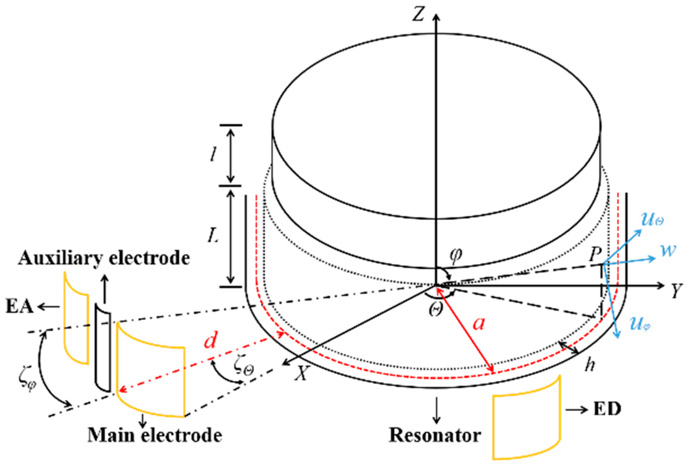
2. Theoretical Analysis

The kinetic energy term in the Lagrangian of a resonator was investigated using the displacement vector components in spherical polar coordinates, as shown in Figure 1. It is specified by giving the components of the displacement vector of a point P on the shell middle surface as a function of the spherical polar coordinates $\phi$ and $\mathrm{\Theta }$. The displacement vector components in spherical polar coordinates are:

$$u_{\phi }(\phi ,\mathrm{\Theta },t)=U_{\phi }(\phi )(w_c(t)\cos 2\mathrm{\Theta }+w_s(t)\sin 2\mathrm{\Theta })$$

(1)

$$u_{\mathrm{\Theta }}(\phi ,\mathrm{\Theta },t)=U_{\mathrm{\Theta }}(\phi )(w_c(t)\sin 2\mathrm{\Theta }-w_s(t)\cos 2\mathrm{\Theta })$$

(2)

$$w(\phi ,\mathrm{\Theta },t)=W(\phi )(w_c(t)\cos 2\mathrm{\Theta }+w_s(t)\sin 2\mathrm{\Theta })$$

(3)

where w_c(t) and w_s(t) are, respectively, the radial components of the displacement vector at the equator at azimuth angles of 0° and 45°.

Considering the generic CVG equations under ideal conditions, where there is no damping, frequency mismatch or other forces and ignoring the centrifugal terms, the Lagrangian of the oscillating cylindrical shell has the form:

$$L=\frac{1}{2}{m}_{eff}({\dot{w}}_c{}^2+{\dot{w}}_s{}^2)+m_{eff}k\mathrm{\Omega }(w_c{\dot{w}}_s-{\dot{w}}_c{w}_s)-\frac{1}{2}{m}_{eff}{\omega }^2(w_c^2+w_s^2)$$

(4)

Among them, $\mathrm{\Omega }$ is the system angular velocity, k is the angular gain, m_eff is the effective mass and $m_{eff}=\frac{f(2)}{8}m$, where f(2) = 1.5296, m is the mass of the shell resonator. More detailed derivations in obtaining the values of m_eff are presented in Appendix A.

When the resonator is driven and read out capacitively, additional forces should be included in the equations of motion. Considering the k_th electrode, which is placed on a spherical surface that is concentric with the shell and centered at ${\phi }_k$ and ${\mathrm{\Theta }}_k$, with angular widths of ${\zeta }_{\phi }$ and ${\zeta }_{\mathrm{\Theta }}$. If we define E as the electromotive force and R as the equivalent circuit resistance [38], we get:

$$R{\dot{q}}_k+\frac{q_k}{C_k}=E$$

(5)

Including the Coriolis and angular acceleration terms, the centrifugal acceleration terms, the damping terms and different natural frequencies of the two modes, the equations of motion satisfied by CVGs have also been listed in Appendix A [39,40,41,42]. Therefore, Lagrange equations are

$$\frac{d}{dt}\frac{\partial L}{\partial {\dot{w}}_c}-\frac{\partial L}{\partial w_c}=0$$

(6)

$$\frac{d}{dt}\frac{\partial L}{\partial {\dot{w}}_s}-\frac{\partial L}{\partial w_s}=0$$

(7)

Firstly, we investigated the electrical contributions to the resonant frequency. Considering the additional electrical potential energy term in the Lagrangian, where $V_{elec}=q_k{}^2/2C_k$, and substituting into (6) and (7), we have:

$$m_{eff}({\ddot{w}}_c+\frac{2}{t}{\dot{w}}_c+{\omega }^2{w}_c)+A+\frac{q_k{}^2}{2C_0}\frac{\partial }{\partial w_c}(\frac{C_0}{C_k})=0$$

(8)

$$m_{eff}({\ddot{w}}_s+\frac{2}{t}{\dot{w}}_s+{\omega }^2{w}_s)+A+\frac{q_k{}^2}{2C_0}\frac{\partial }{\partial w_s}(\frac{C_0}{C_k})=0$$

(9)

A represents the items omitted, the explicit expressions of the values of $\frac{q_k{}^2}{2C_0}\frac{\partial }{\partial w_c}(\frac{C_0}{C_k})$, $\frac{q_k{}^2}{2C_0}\frac{\partial }{\partial w_s}(\frac{C_0}{C_k})$, and A are presented in Appendix B. Substituting these expressions into (8) and (9), we have:

$$\begin{array}{l}{m}_{eff}{\ddot{w}}_c+m_{eff}\left[{\omega }^2-\frac{C_0{E}^2}{2m_{eff}{d}^2}({\gamma }_2-{\gamma }_1{}^2\frac{{\sin }^2{\zeta }_{\mathrm{\Theta }}}{{\zeta }_{\mathrm{\Theta }}{}^2})\right]w_c\\ +m_{eff}(\frac{2}{t}+\frac{1}{R{C}_0\omega }{\gamma }_1{}^2\frac{{\sin }^2{\zeta }_{\mathrm{\Theta }}}{{\zeta }_{\mathrm{\Theta }}{}^2}\frac{C_0{E}^2}{2m_{eff}\omega d^2}){\dot{w}}_c+A=0\end{array}$$

(10)

$$\begin{array}{l}{m}_{eff}{\ddot{w}}_s+m_{eff}\left[{\omega }^2-\frac{C_0{E}^2}{2m_{eff}{d}^2}({\gamma }_2-{\gamma }_1{}^2\frac{{\sin }^2{\zeta }_{\mathrm{\Theta }}}{{\zeta }_{\mathrm{\Theta }}{}^2})\right]w_s\\ +m_{eff}(\frac{2}{t}+\frac{1}{R{C}_0\omega }{\gamma }_1{}^2\frac{{\sin }^2{\zeta }_{\mathrm{\Theta }}}{{\zeta }_{\mathrm{\Theta }}{}^2}\frac{C_0{E}^2}{2m_{eff}\omega d^2}){\dot{w}}_s+A=0\end{array}$$

(11)

Therefore,

$${{\omega }^{\prime }}^2={\omega }^2-\frac{C_0{E}^2}{2m_{eff}{d}^2}({\gamma }_2-{\gamma }_1{}^2\frac{{\sin }^2{\zeta }_{\mathrm{\Theta }}}{{\zeta }_{\mathrm{\Theta }}{}^2})$$

(12)

$$\frac{1}{t^{\prime }}=\frac{1}{t}+\frac{1}{R{C}_0\omega }{\gamma }_1{}^2\frac{{\sin }^2{\zeta }_{\mathrm{\Theta }}}{{\zeta }_{\mathrm{\Theta }}{}^2}\frac{C_0{E}^2}{4m_{eff}\omega d^2}$$

(13)

Similarly, we have

$$\Delta {\omega }^{\prime }=\Delta \omega +({\gamma }_2\frac{\sin 2{\zeta }_{\mathrm{\Theta }}}{2{\zeta }_{\mathrm{\Theta }}}-{\gamma }_1{}^2\frac{{\sin }^2{\zeta }_{\mathrm{\Theta }}}{{\zeta }_{\mathrm{\Theta }}{}^2})\frac{C_0{E}^2}{2m_{eff}\omega d^2}$$

(14)

$$\Delta (\frac{1}{t}{)}^{\prime }=\Delta (\frac{1}{t})+\frac{1}{R{C}_0\omega }{\gamma }_1{}^2\frac{{\sin }^2{\zeta }_{\mathrm{\Theta }}}{{\zeta }_{\mathrm{\Theta }}{}^2}\frac{C_0{E}^2}{2m_{eff}\omega d^2}$$

(15)

where $\omega =\sqrt{\frac{({\omega }_1{}^2+{\omega }_2{}^2)}{2}}$, $\omega \Delta \omega =\frac{{\omega }_2{}^2-{\omega }_1{}^2}{2}$, $\frac{1}{t}=\frac{1}{2}(\frac{1}{t_1}+\frac{1}{t_2})$, and $\Delta (\frac{1}{t})=(\frac{1}{t_2}-\frac{1}{t_1})$. ${\omega }_1$, ${\omega }_2$ are, respectively, the angular frequency of the resonator excited in the low-frequency principal axis and the high-frequency principal axis, while $t_1$, $t_2$ are, respectively, the decay time constant of the resonator excited in the low-damping axis and the high-damping axis.

In addition, the relation between angular frequency and resonant frequency is ${\omega }_1=2\pi f_1$, and the relation between the Q factor and decay time is $Q=\pi f_1{t}_1$[43]. Therefore, ${\omega }_2=2\pi f_2$ and we let $\omega =2\pi f$, $\Delta \omega =2\pi \Delta f$. $f_1$ and $t_1$, in particular, are respectively the resonant frequency and the decay time constant detected in Section 4.

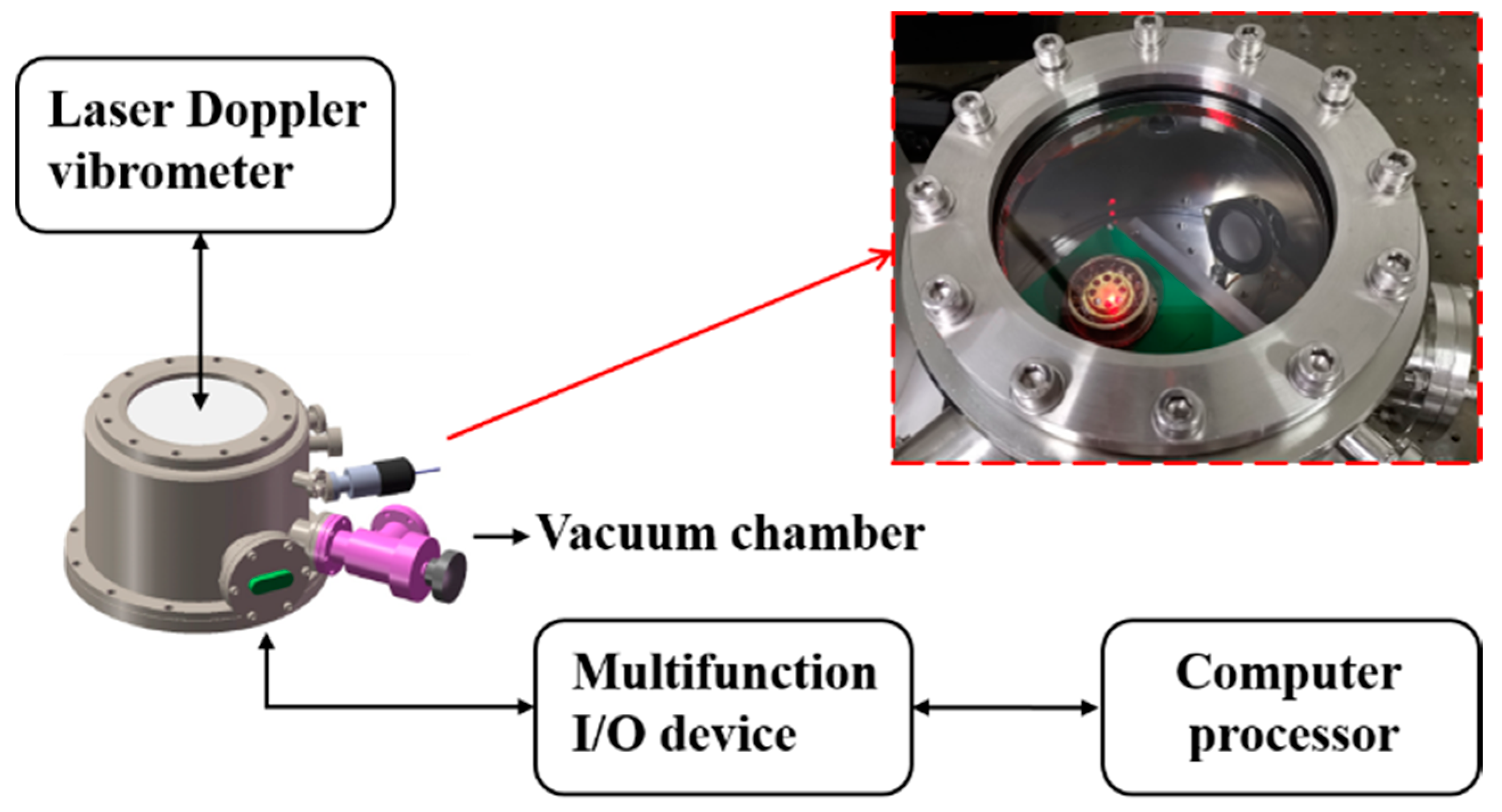
3. Experiments and Methods

Our research group has reported fused silica cylindrical resonators with the Q factor approaching 10⁶ in 2016 [44] and 3 × 10⁶ in 2019 [45]. In this research, a fused silica cylindrical resonator with a high Q factor was fabricated in the same way. For electrostatic excitation and detection, the outer surface of the resonator was coated with Cr/Au (~20/60 nm) film by magnetron sputtering. The resonator was then fixed on a fused silica base through its supporting rod, and a cylindrical ring with laser-cut electrodes was attached on the base outside the resonator. The gap between the resonator and the ring was nearly 20 μm. The main electrodes were used to excite or detect resonator vibration, while the auxiliary electrodes were grounded to reduce signal interference, as shown in Figure 2.

Table 1. Parameters of the resonator and the electrostatic excitation and detection system.

Component	Value	Units
a	1.3 × 10−2	m
d	1.6 × 10−5	m
L	5.7	mm
l	3.1	mm
h	1.2	mm
m	2.8 × 10−3	kg
E	200	V
ζφ	3/13	rad
ζΘ	π/9	rad
φk	π/2–3/26	rad
R	8	GΩ

presents some dimensions of the resonator, as well as some parameters of the electrostatic excitation and detection system, where L and l are, respectively, the height of corresponding cylinders, and h is the width of the resonator. The resonator was characterized in a vacuum chamber with a pressure of 0.01 Pa, and it was placed on an optical table to avoid environmental vibrations.

3.1. Vibrational Characteristics without Electrostatic Influence

For the measurement of the vibrational characteristics without electrostatic influence (VCMs), the resonator system should be isolated from the applied voltage. A laser Doppler vibrometer (Polytec, Irvine, CA, USA) was used to measure the resonant frequency, frequency mismatch, Q factor (decay time), and Q factor asymmetry (decay time split). The resonator was excited by an acoustic source and its vibration detected by the laser Doppler vibrometer. There were material anisotropy and manufacturing errors; therefore, the resonator shows a pair of principal axes of vibration (low-frequency principal axis and high-frequency principal axis), resulting in a natural frequency mismatch. The excitation direction and the low-frequency principal axis had already been aligned in the same orientation before the measurement. The diagram of the experimental setup is shown in Figure 3, and the testing procedure of the VCMs has been described in detail in [16,44,46].

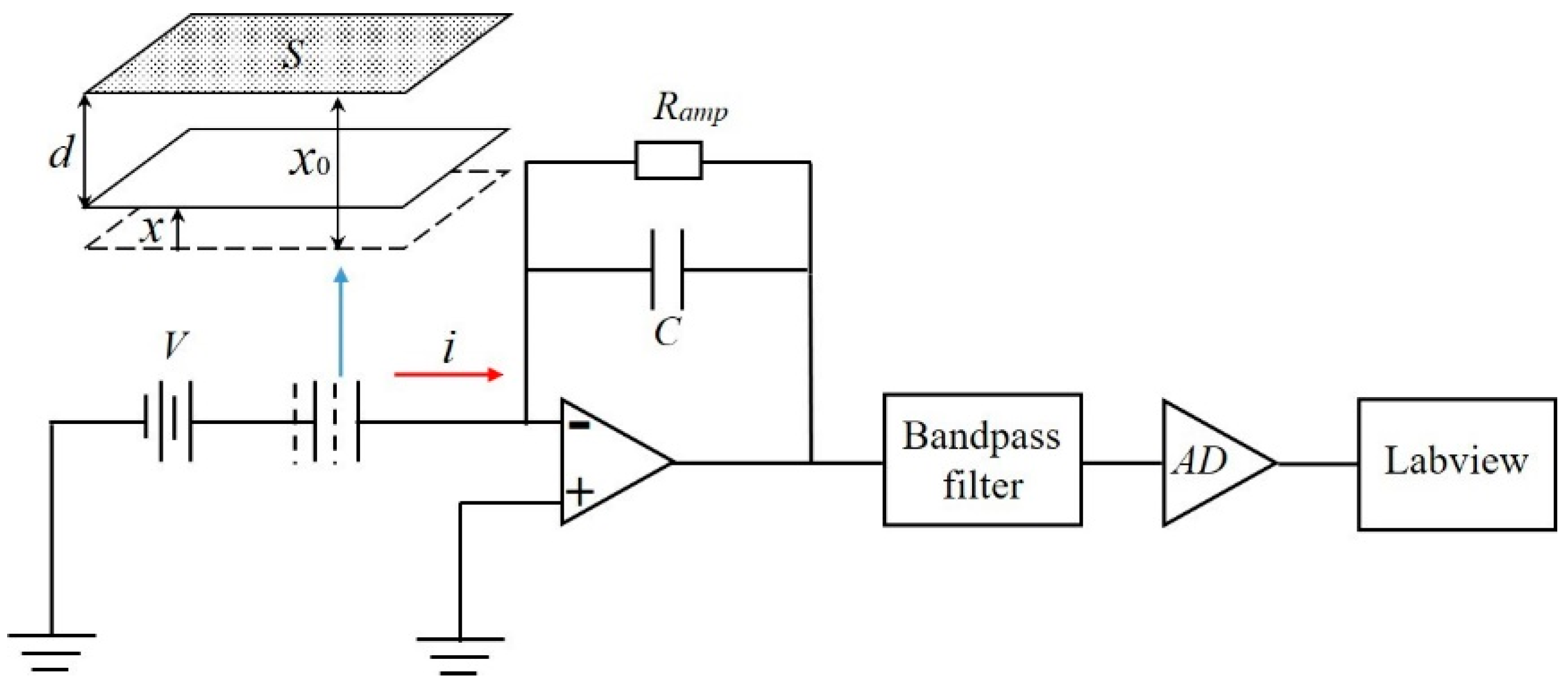
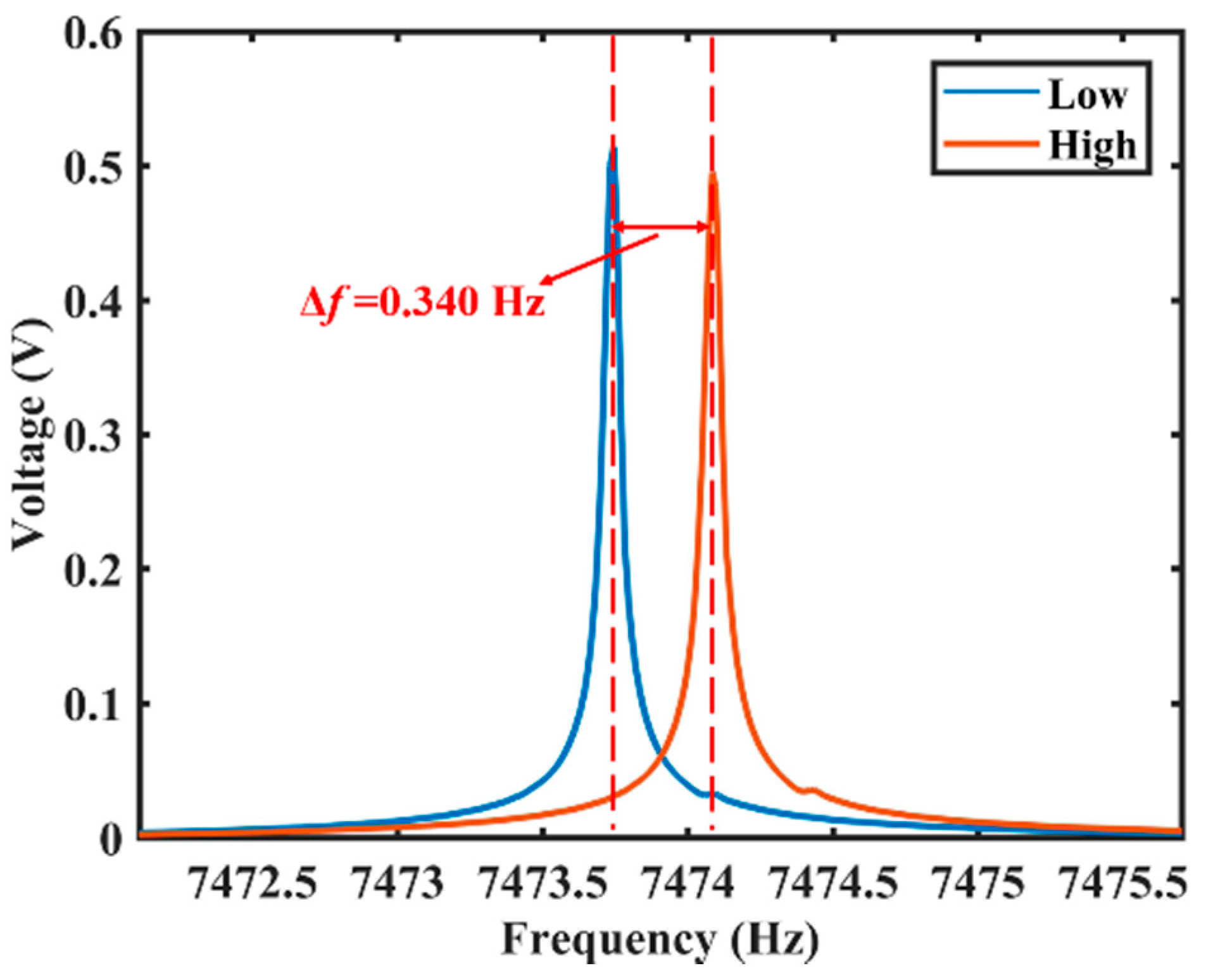
3.2. Vibrational Characteristics with Electrostatic Influence

For the measurement of the vibrational characteristics in practice (VCPs), the resonator system was tested under electrostatic excitation and detection. Electrostatic excitation is based on parallel plate capacitance where the two charged parallel plates produce an attractive force, and the electrostatic force can be obtained by applying an appropriate voltage on the electrodes. Electrostatic detection is also based on parallel plate capacitance where the two movable plates can charge or discharge, hence producing a measurable current for the following conditioning circuits [47]. The outside surface of the resonator and the main electrodes formed parallel plate capacitors, which were used to excite or detect the displacement of the resonator from different directions. Figure 4 shows the schematic of electrostatic detection, including the C/V converter, bandpass filter, analog to digital (AD) converter, and LabVIEW process program. The upper plate represents one of the main electrodes and the bottom plate represents the outside surface of the resonator.

The capacitance for a parallel plate capacitor is [48]:

$$C=\frac{\epsilon S}{d}$$

(16)

where $\epsilon$ is the permittivity of the material between two movable plates, S is the area of the plates, d is the actual gap when the resonator vibrates, x₀ is the initial gap between two movable plates, and x is the displacement of the bottom plate. A variation in the gap between two movable plates causes a variation in the capacitance, resulting in the variation of the current. The series expansion of the current i around x = 0 is:

$$i=\frac{\epsilon S}{x_0{}^2}V\dot{x}+2\frac{\epsilon S}{x_0{}^3}Vx\dot{x}+o(x^2)$$

(17)

where V is the high DC voltage applied to the resonator. Because the magnitude of the resonant surface x is far less than the initial gap x₀, the higher-order terms o(x²) are negligible. Substitute $x=a\sin \omega t$ into (17); the cross term $x\dot{x}$ splits into a DC component and a $2\omega$ frequency component, which can both be eliminated by the bandpass filter. The output current signal is

$$i=\frac{\epsilon S}{x_0{}^2}Va\omega \cos \omega t$$

(18)

The output voltage signal is then:

$$U=R_{amp}\frac{\epsilon S}{x_0{}^2}Va\omega \cos \omega t$$

(19)

where R_amp is the resistance.

Using a multifunction I/O device, the actuating capacitors were connected to voltage sources. Excitation signals were generated by the multifunction I/O device with the controlled program designed and operated in the LabVIEW software, and all the relative parameters could be easily adjusted. Detection signals from sensing capacitors were collected by the multifunction I/O device and processed by the LabVIEW program, as shown in Figure 3.

The testing procedure of the VCPs was as follows. A pair of ring electrodes EA, along with the low-frequency principal axis was used for actuation, while the pair ED in quadrature with EA was used for detection. A sweeping voltage signal was applied to EA and the sweeping frequency data was recorded from ED. The resonant frequency f was then obtained through Fast Fourier transform. As for Q factor measurement, a sinusoidal voltage signal with the resonant frequency was applied to EA, and the signal was then cut off., and the ring-down time was recorded. The measurement for the resonant frequency and decay time was repeated for the high-frequency principal axis; hence, the frequency mismatch and the decay time split were acquired.

4. Results and Discussion

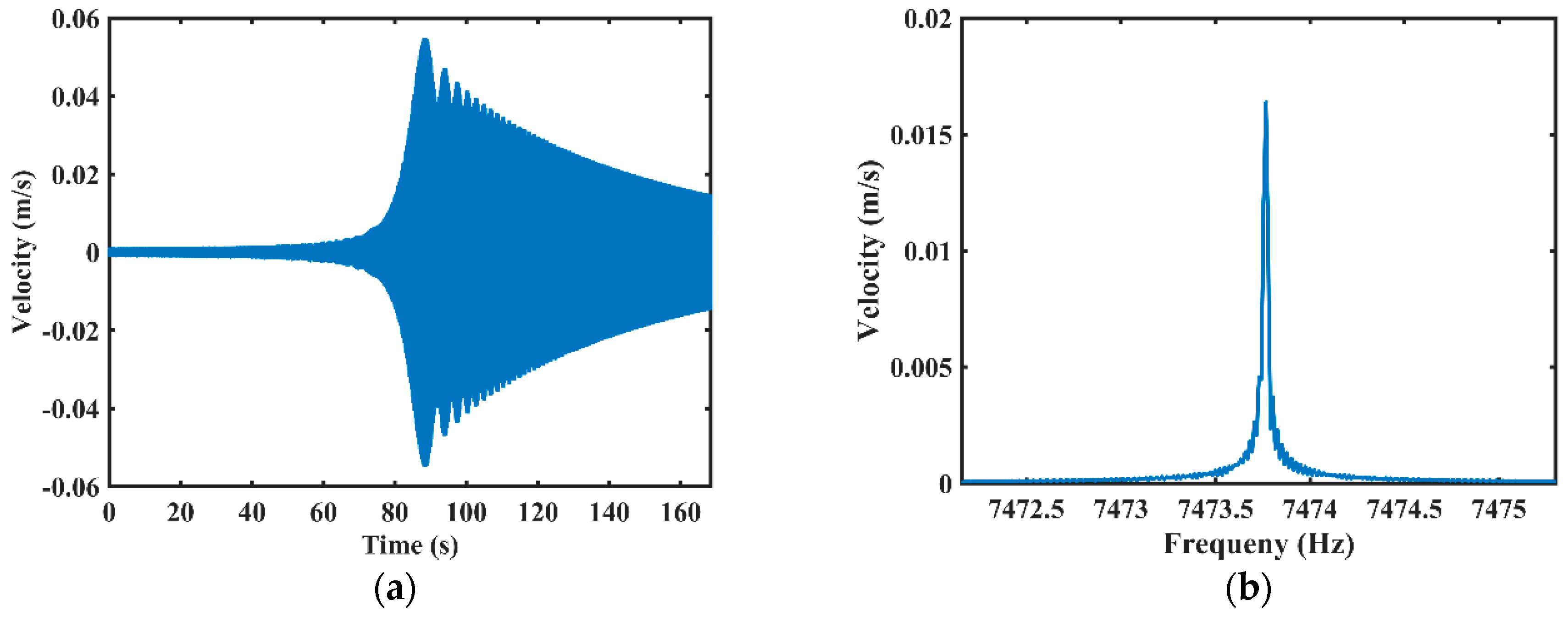
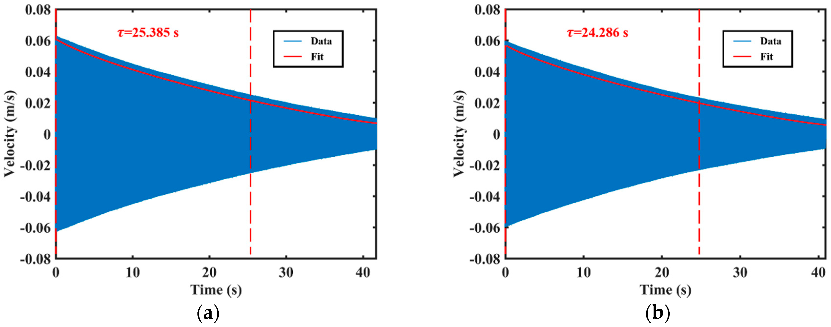
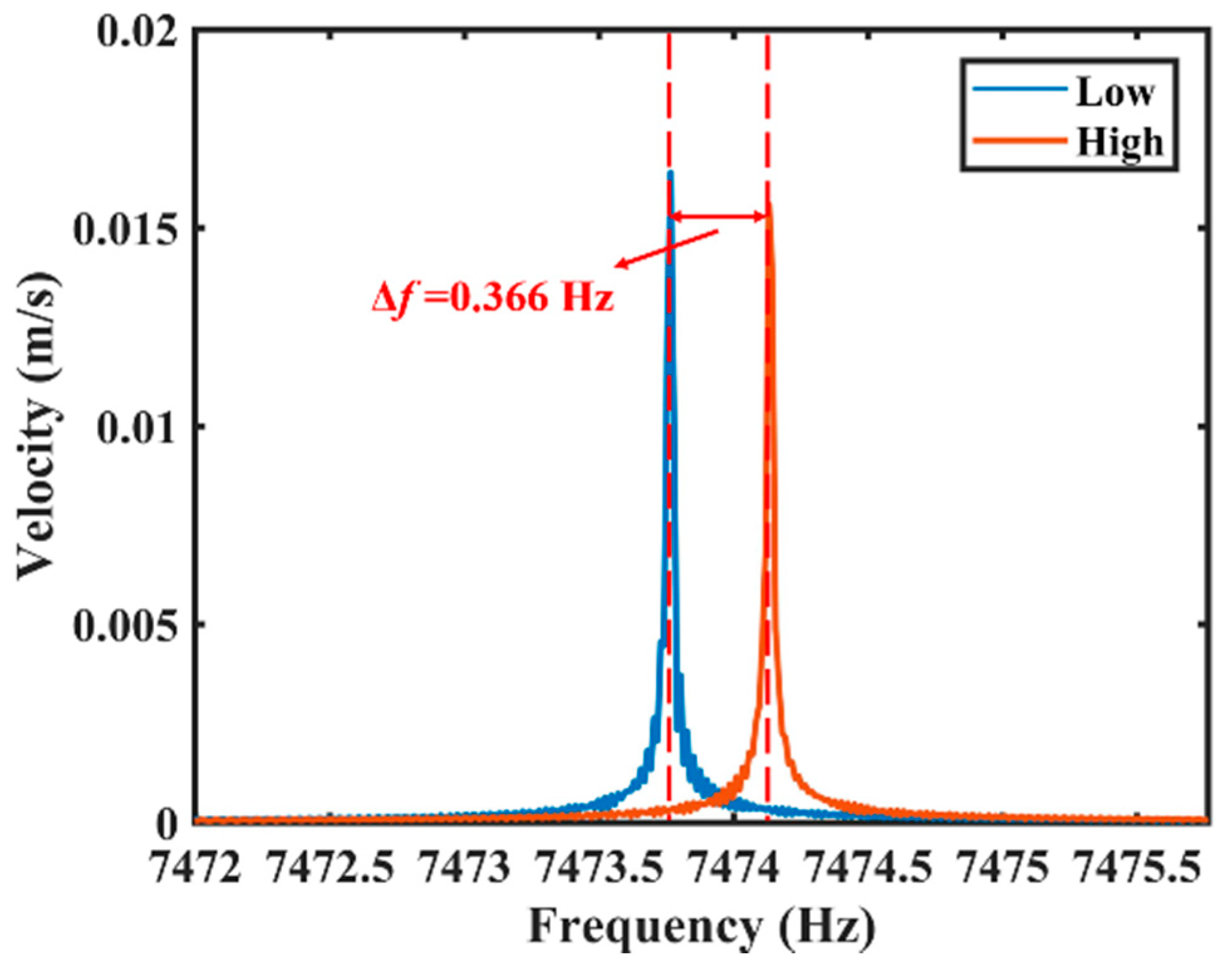
4.1. Vibrational Characteristics in Measurements

Table 2. The VCMs detected by the laser Doppler vibrometer.

Component	Frequency (Hz)	Decay Time (s)	Q Factor
1	7473.767	25.385	5.960 × 105
2	7474.133	24.286	5.703 × 105
Δ	0.366	1.099	2.578 × 104

presents all the VCMs detected by the laser Doppler vibrometer. Series 1 represents the VCMs excited in the low-frequency principal axis. Series 2 represents the VCMs excited in the high-frequency principal axis. Series Δ represents the variations between Series 1 and Series 2.

The sweeping measurements detected by the laser Doppler vibrometer are shown in Figure 5. When applying a sweeping signal to the acoustic source, the resonator was excited and gradually reached the maximum value, about 55 mm/s, as shown in Figure 5a. Then, the vibration velocity gradually decayed as the frequency of the excitation signal deviated from the resonant frequency. The sweeping frequency data was processed by a Fast Fourier Transform (FFT) program, and the resonant frequency is about 7473.767 Hz, as shown in Figure 5b.

The ring-down time measurement results are shown in Figure 6. The decay time constant of the resonator (low-frequency axis excited) is about 25.385 s, as shown in Figure 6a. The Q factor is approximately 5.960 × 10⁵, calculated by the equation described in [43]. Similarly, the resonant frequency of the high-frequency principal axis was measured to be about 7474.133 Hz, the decay time constant was about 24.286 s, as shown in Figure 6b. The Q factor is approximately 5.703 × 10⁵.

The variation of the decay time is about 1.099 s, and the variation of the Q factor is about 2.578 × 10⁴. The frequency mismatch of the resonator is about 0.366 Hz, as shown in Figure 7.

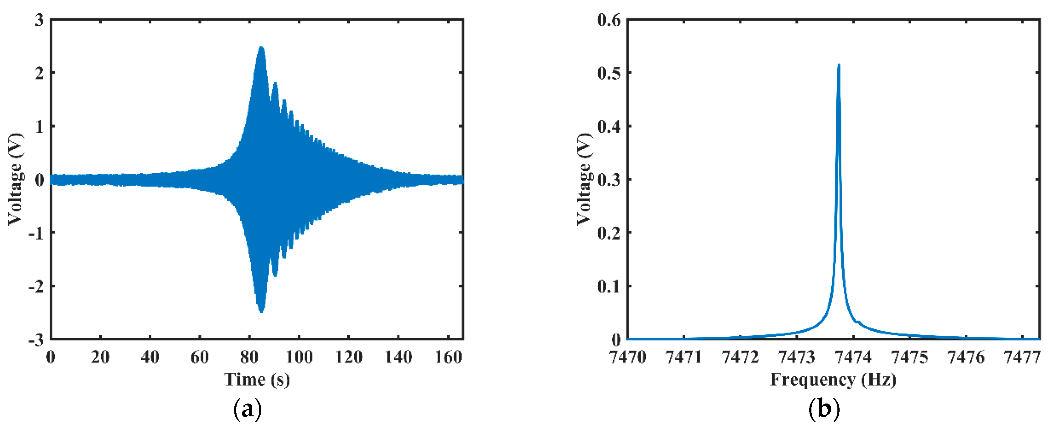
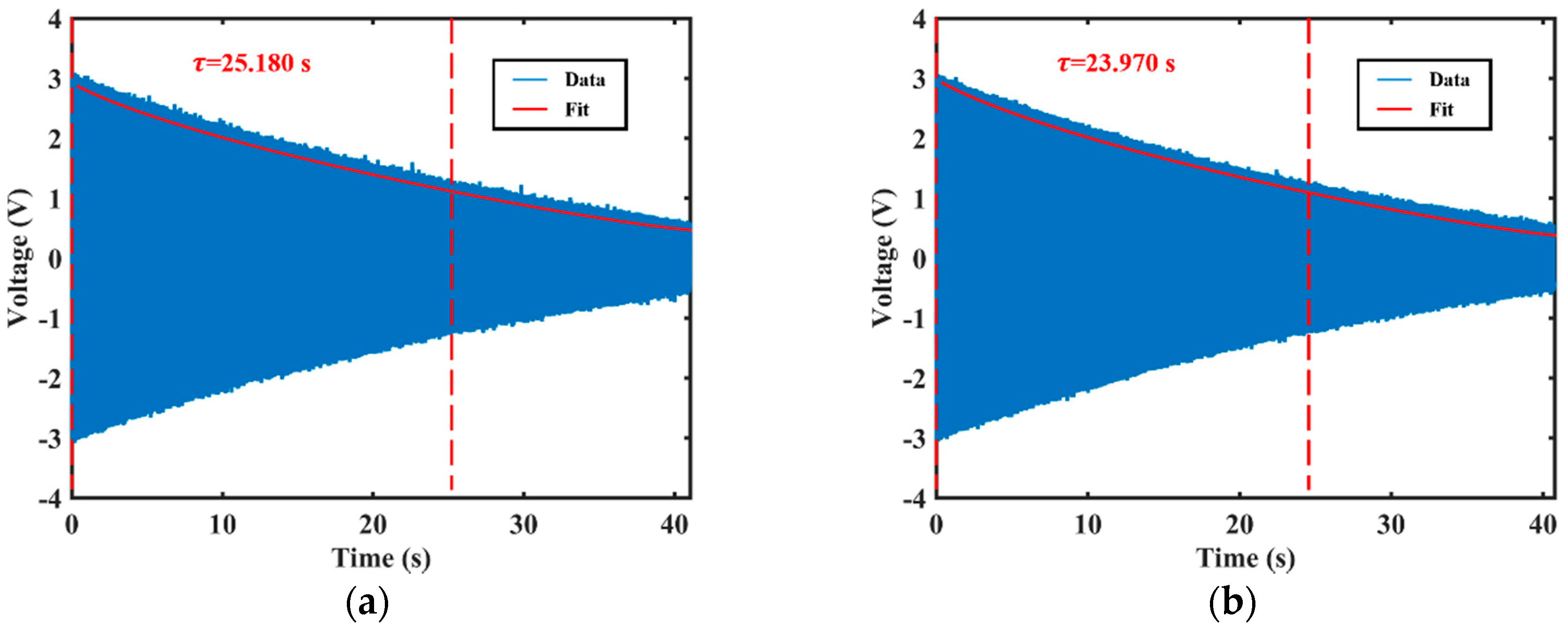
4.2. Vibrational Characteristics in Practice

Table 3. The VCPs detected by electrostatic excitation and detection.

Component	Frequency (Hz)	Decay Time (s)	Q Factor
1	7473.745	25.180	5.912 × 105
2	7474.085	23.970	5.628 × 105
Δ	0.340	1.210	2.838 × 104

presents all the VCPs detected by electrostatic excitation and detection. Series 1 represents the VCPs excited in the low-frequency principal axis. Series 2 represents the VCPs excited in the high-frequency principal axis. Series Δ represents the variations between Series 1 and Series 2.

The sweeping measurements detected by electrostatic excitation and detection are shown in Figure 8. When applying a sweeping signal to EA, the output voltage signal of ED reached its maximum magnitude, about 2.5 V, as shown in Figure 8a. Then, the output voltage signal of ED gradually decayed as the frequency of the excitation signal deviated from the resonant frequency. The sweeping frequency data was processed by an FFT program, and the resonant frequency is about 7473.745 Hz, as shown in Figure 8b.

The ring-down time measurement results are shown in Figure 9. The decay time constant of the resonator (low-frequency axis excited) is about 25.180 s, as shown in Figure 9a. The Q factor is approximately 5.912 × 10⁵. Similarly, the resonant frequency of the high-frequency principal axis was about 7474.085 Hz, the decay time constant was about 23.970 s, as shown in Figure 9b. The Q factor is approximately 5.628 ×10⁵.

The variation of the decay time is about 1.210 s, and the variation of the Q factor is about 2.838 × 10⁴. The frequency mismatch of the resonator is about 0.340 Hz, as shown in Figure 10.

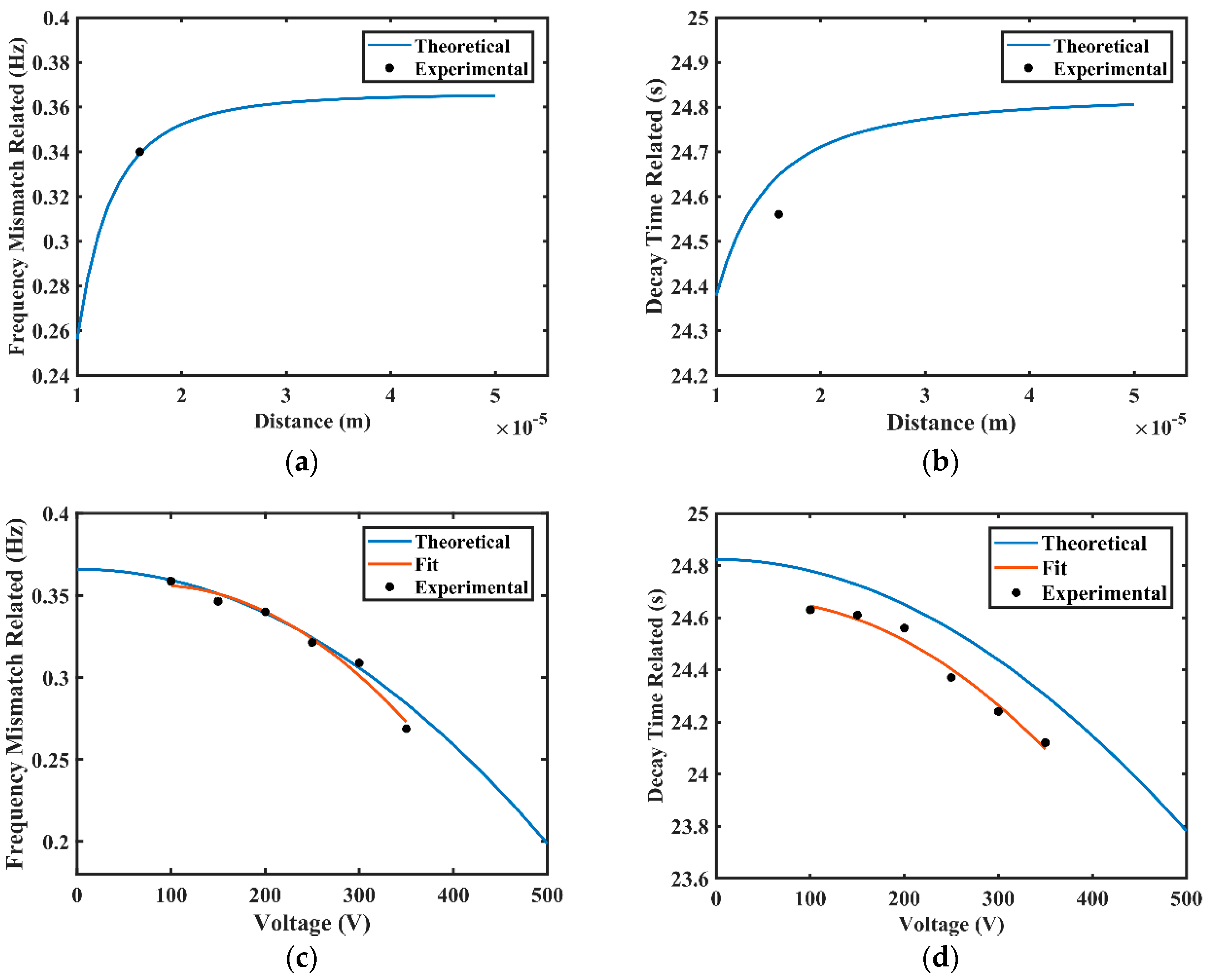
4.3. Results and Comparisons between Analysis and Experiments

Table 4. Results and comparisons between the VCMs and the VCPs.

Component	VCMs	VCPs	Variation
f1 (Hz)	7473.767	7473.745	−0.022
f2 ‒ f1 (Hz)	0.366	0.340	−0.026
t1 (s)	25.385	25.180	−0.205
t2 ‒ t1 (s)	1.099	1.210	0.111

presents the results and comparisons between the measured VCMs and the VCPs, where f₁ is the resonant frequency of the low-frequency principal axis, t₁ is the decay time, f₂ ‒ f₁ is the frequency mismatch, and t₂ ‒ t₁ is the decay time split. The resonant frequency in measurements and in practice of the resonator are, respectively, 7473.767 Hz and 7473.745 Hz, which decreases by 0.022 Hz. The frequency mismatch in measurements and in practice are respectively 0.366 Hz and 0.340 Hz, which decreases 0.026 Hz. The decay time in measurements and in practice are, respectively, 25.385 s and 25.180 s, which decreases by 0.205 s. The decay time split in measurements, and in practice are, respectively, 1.099 s to 1.210 s, which increases 0.111 s. Therefore, electrostatic forces do have an influence on vibrational characteristics, and the influence is relatively minor but still cannot be ignored.

Table 5. Results and comparisons among the theoretical vibrational characteristics, the VCPs, and the VCMs.

Component	VCMs	VCPs	Variation 1	Theoretical	Variation 2
f (Hz)	7473.950	7473.915	−0.035	7473.927	−0.023
$\Delta f$(Hz)	0.366	0.340	−0.026	0.339	−0.027
$\frac{1}{t}$(s−1)	0.0403	0.0407	0.0004	0.0406	0.0003
$\Delta (\frac{1}{t})$(s−1)	0.0018	0.0020	0.0002	0.0023	0.0005

presents all the results and comparisons between the VCMs and the theoretical vibrational characteristics, and between the VCMs and the VCPs. Using the vibrational characteristics listed in Table 3, the corresponding f, $\Delta f$, $\frac{1}{t}$, and $\Delta (\frac{1}{t})$ in practice can be calculated, and the comparisons between the VCMs and the VCPs are listed in Variation 1. With parameters in Table 1 and the measured resonant frequency without electrostatic influence, we can calculate the ${\omega }^{\prime }$ according to Equation (12). Therefore, when the resonant frequencies in measurements of the resonator are respectively 7473.767 Hz and 7474.133 Hz in two axes, f equals to 7473.950 Hz, and the theoretical result f ‘ equals to 7473.927 Hz, which decreased by 0.023 Hz. According to Equation (14), when the $\Delta f$ in measurements of the resonator is 0.366 Hz, the theoretical result $\Delta f^{\prime }$ equals to 0.339 Hz, which decreased by 0.027 Hz. According to Equation (13), when the decay time in measurements of the resonator are respectively 25.385 s and 24.286 s in two axes, $\frac{1}{t}$ equals to 0.0403 s^−1, and the theoretical result $\frac{1}{t^{\prime }}$ equals to 0.0406 s⁻¹, which increased 0.0003 s⁻¹. According to Equation (15), $\Delta (\frac{1}{t})$ equals to 0.0018 s⁻¹, and the theoretical result $\Delta (\frac{1}{t}{)}^{\prime }$ equals to 0.0023 s⁻¹, which increased 0.0005 s⁻¹. Comparing Variation 1 with Variation 2, the variation trends of f, $\Delta f$, $\frac{1}{t}$, and $\Delta (\frac{1}{t})$ measured in experiments are all consistent with calculations.

According to the theoretical analysis, $\Delta f^{\prime }$ and $t^{\prime }$ vary with the distance between two electrodes, as shown in Figure 11a,b. As the distance between two electrodes varying from 1 × 10⁻⁵ m to 5 × 10⁻⁵ m, the frequency mismatch related $\Delta f^{\prime }$ gradually rises from 0.260 Hz to 0.362 Hz (increased by 39.23%), and the decay time related $t^{\prime }$ gradually rises from 24.38 s to 24.80 s (increased by 1.72%). Therefore, higher distance results in higher frequency mismatch and higher decay time. As the gyroscope performance degrades, when the frequency mismatch increases and decay time decreases [10], the distance between two electrodes should be set to an appropriate value for a given structure. In addition, $\Delta f^{\prime }$ and $t^{\prime }$ also vary with the applied voltage, as shown in Figure 11c,d. When the applied voltage varies from 0 V to 500 V, the frequency mismatch $\Delta f^{\prime }$ gradually decreases from 0.366 Hz to 0.205 Hz (decreased by 43.99%), and $t^{\prime }$ gradually decreases from 24.82 s to 23.78 s (decreased by 4.19%). Therefore, higher applied voltage results in lower frequency mismatch and lower decay time, the applied voltage should be optimized for a given structure. The frequency mismatch related $\Delta f$ and the decay time-related t in practice were tested under different applied voltages, and the results are shown in

Table 6. The frequency mismatch related $\Delta f$ and the decay time-related t in practice varying with the applied voltage.

Voltage (V)	$\Delta \mathit{f}\left(\mathbf{Hz}\right)$	t (s)
100	0.359	24.630
150	0.346	24.610
200	0.340	24.560
250	0.321	24.370
300	0.309	24.240
350	0.279	24.120

. Experimental results are also displayed in Figure 11, which show good agreement with theoretical calculations.

5. Conclusions

This paper reports the experimental results on the changes of resonant frequency, frequency mismatch, decay time, and decay time split under electrostatic forces. Experiments were performed on a film-coated fused quartz cylindrical resonator with ring electrodes. Compared with results measured by Laser Doppler vibrometer, these parameters changed slightly with electrostatic excitation and detection. With the influence of electrostatic forces, the resonant frequency decreased by 0.022 Hz, the frequency mismatch decreased by 0.026 Hz, the decay time decreased by 0.205 s, and the decay time split increased by 0.111 s. These changes were theoretically analyzed by introducing electrostatic force into dynamic equations of the Coriolis vibratory gyroscope, and variation trends in experimental results were consistent with the theoretical analysis. The change of the frequency split and decay time with the capacitive gap and the applied voltage were estimated, and the change of the frequency split and decay time were tested under different applied voltages. Lower capacitive gaps and larger applied voltages result in lower frequency mismatch and lower decay time. Therefore, the capacitive gap and applied voltage should be appropriately designed to improve gyroscope performance.

References

1. Chikovani, V.; Okon, I.; Barabashov, A.; Tewksbury, P. A set of high accuracy low cost metallic resonator CVG. In Proceedings of the 2008 IEEE/ION Position, Location and Navigation Symposium, Monterey, CA, USA, 5–8 May 2008; pp. 238–243. [Google Scholar]
2. Chikovani, V.; Yatsenko, Y.A.; Barabashov, A.; Marusyk, P.; Umakhanov, E.; Taturin, V.J.I.A.; Magazine, E.S. Improved accuracy metallic resonator CVG. IEEE Aerosp. Electron. Syst. Mag. 2009, 24, 40–43. [Google Scholar] [CrossRef]
3. Yatsenko, Y.A.; Petrenko, S.; Vovk, V.; Chikovani, V. Technological aspects of manufacturing of compound hemispherical resonators for small-sized vibratory gyroscopes. In Proceedings of the 6th Saint Petersburg International Conference on Integrated Navigation Systems, St. Petersburg, Russia, 24–26 May 1999. [Google Scholar]
4. Rozelle, D.M. The hemispherical resonator gyro: From wineglass to the planets. In Proceedings of the 19th AAS/AIAA Space Flight Mechanics Meeting, Savannah, Georgia, 8–12 February 2009; pp. 1157–1178. [Google Scholar]
5. Watson, W.S. Vibratory gyro skewed pick-off and driver geometry. In Proceedings of the IEEE/ION Position, Location and Navigation Symposium, Indian Wells, CA, USA, 4–6 May 2010; pp. 171–179. [Google Scholar]
6. Sarapuloff, S. Development and cost reduction of high-Q dielectric resonators of solid-state gyroscopes. In Proceedings of the 8th Saint Petersburg International Conference on Integrated Navigation Systems, St. Petersburg, Russia, 28–30 May 2001; pp. 124–126. [Google Scholar]
7. Sarapuloff, S. Dynamics of Precise Solid-State Gyroscopes of HRG and CRG Types. In Proceedings of the V-th Brazilian Symposium on Inertial Engineering (V SBEIN), Rio de Janeiro, Brazil, 27–29 November 2007; pp. 27–29. [Google Scholar]
8. Chikovani, V.V.; Yatzenko, Y.A.; Kovalenko, V.A. Coriolis Force Gyroscope with High Sensitivity. U.S. Patent 7513156B2, 7 April 2009. [Google Scholar]
9. Northrop Grumman Corporation. Available online: http://www.globenewswire.com/newsarchive/noc/press/pages/news_releases.html?d=10120447 (accessed on 5 September 2019).
10. Zhang, F. Control and Self-Calibration of Microscale Rate Integrating Gyroscopes (MRIGs); UC Berkeley: Berkeley, CA, USA, 2015. [Google Scholar]
11. Rozelle, D.; Meyer, A.; Trusov, A.; Sakaida, D. Milli-HRG inertial sensor assembly–a reality. In Proceedings of the 2015 IEEE International Symposium on Inertial Sensors and Systems (ISISS) Proceedings, Hapuna Beach, HI, USA, 23–26 March 2015; pp. 1–4. [Google Scholar]
12. Jeanroy, A.; Grosset, G.; Goudon, J.-C.; Delhaye, F. HRG by Sagem from laboratory to mass production. In Proceedings of the 2016 IEEE International Symposium on Inertial Sensors and Systems, Laguna Beach, CA, USA, 22–25 Febuary 2016; pp. 1–4. [Google Scholar]
13. Jeanroy, A.; Bouvet, A.; Remillieux, G.J.G.; Navigation. HRG and marine applications. Gyroscopy Navig. 2014, 5, 67–74. [Google Scholar] [CrossRef]
14. Waston Industries. Available online: https://watson-gyro.com/product/rate-gyros/pro-gyro-rate-gyro/ (accessed on 27 August 2019).
15. Innalabs. Available online: http://www.innalabs.com/en/products/gyroscopes/ (accessed on 5 September 2019).
16. Qiu, Z.; Qu, T.; Pan, Y.; Jia, Y.; Fan, Z.; Yang, K.; Yuan, J.; Luo, H.J.S. Optical and Electrical Method Characterizing the Dynamic Behavior of the Fused Silica Cylindrical Resonator. Sensors 2019, 19, 2928. [Google Scholar] [CrossRef] [PubMed] [Green Version]
17. Lee, E.Y.; Sensors, A.A.S.J.; Physical, A.A. 5.4-MHz single-crystal silicon wine glass mode disk resonator with quality factor of 2 million. Sens. Actuators A Phys. 2009, 156, 28–35. [Google Scholar] [CrossRef]
18. Elsayed, M.Y.; Nabki, F. 18-MHz Silicon Lamé Mode Resonators With Corner and Central Anchor Architectures in a Dual-Wafer SOI Technology. J. Microelectromech. Syst. 2017, 26, 67–74. [Google Scholar] [CrossRef]
19. Khine, L.; Palaniapan, M.; Wong, W.K. 6 MHz Bulk-Mode Resonator with Q Values Exceeding One Million. In Proceedings of the TRANSDUCERS 2007—2007 International Solid-State Sensors, Actuators and Microsystems Conference, Lyon, France, 10–14 June 2007. [Google Scholar]
20. Elsayed, M.Y.; Nabki, F. 870 000$ Q $-Factor Capacitive Lamé Mode Resonator With Gap Closing Electrodes Enabling 4.4 k $\Omega $ Equivalent Resistance at 50 V. IEEE Trans. Ultrason. Ferroelectr. Freq. Control 2019, 66, 717–726. [Google Scholar] [CrossRef]
21. Johari, H.; Ayazi, F. High-frequency capacitive disk gyroscopes in (100) and (111) silicon. In Proceedings of the IEEE International Conference on Micro Electro Mechanical Systems, Hyogo, Japan, 21–25 January 2007. [Google Scholar]
22. Cicek, P.V.; Elsayed, M.; Nabki, F.; El-Gamal, M. A novel multi-level IC-compatible surface microfabrication technology for MEMS with independently controlled lateral and vertical submicron transduction gaps. J. Micromech. Microeng. 2017, 27, 115002. [Google Scholar] [CrossRef] [Green Version]
23. Nabki, F.; Elsayed, M.Y.; El-Gamal, M.N. A combined comb/bulk mode gyroscope structure for enhanced sensitivity. In Proceedings of the IEEE International Conference on Micro Electro Mechanical Systems, Taipei, Taiwan, 20–24 January 2013. [Google Scholar]
24. Elsayed, M.Y.; Nabki, F. Piezoelectric Bulk Mode Disk Resonator Post-Processed for Enhanced Quality Factor Performance. J. Micromech. Microeng. 2017, 26, 75–83. [Google Scholar] [CrossRef]
25. Piazza, G.; Stephanou, P.J.; Pisano, A.P. Piezoelectric Aluminum Nitride Vibrating Contour-Mode MEMS Resonators. J. Micromech. Microeng. 2006, 15, 1406–1418. [Google Scholar] [CrossRef] [Green Version]
26. Gong, S.; Piazza, G. Design and Analysis of Lithium–Niobate-Based High Electromechanical Coupling RF-MEMS Resonators for Wideband Filtering. IEEE Trans. Microw. Theory Tech. 2013, 61, 403–414. [Google Scholar] [CrossRef]
27. Thakar, V.; Rais-Zadeh, M. Temperature-compensated piezoelectrically actuated Lamé-mode resonators. In Proceedings of the 2014 IEEE 27th International Conference on Micro Electro Mechanical Systems (MEMS), San Francisco, CA, USA, 26–30 January 2014. [Google Scholar]
28. Green, E.I. The story of Q. Am. Sci. 1955, 43, 584–594. [Google Scholar]
29. Painter, C.C.; Shkel, A.M. Active structural error suppression in MEMS vibratory rate integrating gyroscopes. IEEE Sens. J. 2003, 3, 595–606. [Google Scholar] [CrossRef] [Green Version]
30. Gallacher, B.J.; Hedley, J.; Burdess, J.S.; Harris, A.J.; Rickard, A.; King, D.O. Electrostatic correction of structural imperfections present in a microring gyroscope. J. Micromech. Syst. 2005, 14, 221–234. [Google Scholar] [CrossRef]
31. Ahn, C.H.; Ng, E.J.; Hong, V.A.; Yang, Y.; Lee, B.J.; Flader, I.; Kenny, T.W. Mode-matching of wineglass mode disk resonator gyroscope in (100) single crystal silicon. J. Micromech. Syst. 2014, 24, 343–350. [Google Scholar] [CrossRef]
32. Asadian, M.H.; Wang, Y.; Askari, S.; Shkel, A. Controlled capacitive gaps for electrostatic actuation and tuning of 3D fused quartz micro wineglass resonator gyroscope. In Proceedings of the 2017 IEEE International Symposium on Inertial Sensors and Systems (INERTIAL), Kauai, HI, USA, 27–30 March 2017; pp. 1–4. [Google Scholar]
33. Hu, Z.; Gallacher, B.J. Precision mode tuning towards a low angle drift MEMS rate integrating gyroscope. Mechatronics 2018, 56, 306–317. [Google Scholar] [CrossRef] [Green Version]
34. Darvishian, A.; Boyd, C.; Singh, S.; Cho, J.-Y.; Woo, J.-K.; He, G.; Najafi, K. Effect of Electrode Design on Frequency Tuning in Shell Resonators. In Proceedings of the 2019 IEEE International Symposium on Inertial Sensors and Systems (INERTIAL), Naples, FL, USA, 1–5 April 2019; pp. 1–4. [Google Scholar]
35. Zotov, S.A.; Simon, B.R.; Prikhodko, I.P.; Trusov, A.A.; Shkel, A.M. Quality Factor Maximization Through Dynamic Balancing of Tuning Fork Resonator. IEEE Sens. J. 2014, 14, 2706–2714. [Google Scholar] [CrossRef]
36. Trusov, A.A.; Zotov, S.A.; Shkel, A.M. Electrostatic regulation of quality factor in non-ideal tuning fork MEMS. In Proceedings of the 2011 IEEE Sensors, Limerick, Ireland, 28–31 October 2011. [Google Scholar]
37. Cheng, P.; Zhang, Y.; Gu, W.; Hao, Z.J.S.; Physical, A.A. Effect of polarization voltage on the measured quality factor of a multiple-beam tuning-fork gyroscope. Sens. Actuators A Phys. 2012, 187, 118–126. [Google Scholar] [CrossRef]
38. Zhuravlev, V.F.; Lynch, D.D. Electric model of a hemispherical resonator gyro. Mech. Solids 1995, 30, 10–21. [Google Scholar]
39. Lynch, D. Coriolis vibratory gyros. In Proceedings of the Symposium Gyro Technology, Stuttgart, Germany, 15–16 September 1998. [Google Scholar]
40. Lynch, D.D. Vibratory gyro analysis by the method of averaging. In Proceedings of the 2nd St. Petersburg Conference on Gyroscopic Technology and Navigation, St. Petersburg, Russia, 24–25 May 1995; pp. 26–34. [Google Scholar]
41. Liu, N.; Su, Z.; Liu, H. Research on the control loop for Solid Vibratory Gyroscope. In Proceedings of the 32nd Chinese Control Conference, Xi’an, China, 26–28 July 2013; pp. 4963–4968. [Google Scholar]
42. Wang, X.; Wu, W.; Luo, B.; Fang, Z.; Li, Y.; Jiang, Q.J.S. Force to rebalance control of HRG and suppression of its errors on the basis of FPGA. Sensors 2011, 11, 11761–11773. [Google Scholar] [CrossRef]
43. Zhang, M.; Llaser, N.; Rodes, F. High-precision time-domain measurement of quality factor. IEEE Trans. Instrum. Meas. 2011, 61, 842–844. [Google Scholar] [CrossRef]
44. Pan, Y.; Wang, D.; Wang, Y.; Liu, J.; Wu, S.; Qu, T.; Yang, K.; Luo, H.J.S. Monolithic cylindrical fused silica resonators with high Q factors. Sensors 2016, 16, 1185. [Google Scholar] [CrossRef] [PubMed] [Green Version]
45. Luo, Y.; Qu, T.; Cui, Y.; Pan, Y.; Yu, M.; Luo, H.; Jia, Y.; Tan, Z.; Liu, J.; Zhang, B. Cylindrical Fused Silica Resonators Driven by PZT Thin Film Electrodes with Q Factor Achieving 2.89 Million after Coating. Sci. Rep. 2019, 9, 9461. [Google Scholar] [CrossRef] [PubMed]
46. Luo, Y.; Qu, T.; Zhang, B.; Pan, Y.; Xiao, P. Simulations and Experiments on the Vibrational Characteristics of Cylindrical Shell Resonator Actuated by Piezoelectric Electrodes with Different Thicknesses. Shock Vib. 2017, 2017, 2314858. [Google Scholar] [CrossRef] [Green Version]
47. Nair, B.S.; Deepa, S. Applied Electromagnetic Theory: Analyses, Problems and Applications; PHI Learning Pvt. Ltd.: Delhi, India, 2008. [Google Scholar]
48. Senkal, D. Micro-glassblowing Paradigm for Realization of Rate Integrating Gyroscopes. Ph.D. Thesis, University of California, Irvine, CA, USA, 2015. [Google Scholar]
49. Rayleigh, J.W.S.B. The Theory of Sound; Macmillan: New York, NY, USA, 1896; Volume 2. [Google Scholar]
50. Zhuravlev, V.F. Theoretical principles of a solid state wave gyroscope. Ross. Akad. Nauk Izv. Mekhanika Tverd. Tela 1993, 28, 6–19. [Google Scholar]
Figure 1. Schematic diagram of the resonator coordinate.
Sensors 20 00295 g001
Figure 2. The sectional view of the resonator and the electrodes.
Sensors 20 00295 g002
Figure 3. The diagram of the experimental setup used for the testing of both the VCMs and the VCPs.
Sensors 20 00295 g003
Figure 4. The schematic of the electrostatic detection.
Sensors 20 00295 g004
Figure 5. The results of the sweeping frequency detected by the laser Doppler vibrometer: (a) The vibration velocity detected by the laser Doppler vibrometer; (b) Fast Fourier transform (FFT) results of the vibration velocity.
Sensors 20 00295 g005
Figure 6. The decay time constant measured by ring-down time method: (a) The decay time constant excited by the low-frequency principal axis; (b) The decay time constant excited by the high-frequency principal axis.
Sensors 20 00295 g006
Figure 7. The FFT results of the vibration velocity of two vibrating modes with different frequencies. The blue line represents exciting in the direction of the low-frequency principal axis, and the red line represents exciting in the direction of the high-frequency principal axis.
Sensors 20 00295 g007
Figure 8. The results of frequency sweeping detected by electrostatic excitation and detection: (a) The output voltage signal of the ED; (b) Fast Fourier transform (FFT) results of the output voltage signal.
Sensors 20 00295 g008
Figure 9. The decay time constant measured by ring-down time method: (a) The decay time constant excited by the low-frequency axis; (b) The decay time constant excited by the high-frequency axis.
Sensors 20 00295 g009
Figure 10. The FFT results of the output voltage signal of two vibrating modes with different frequencies. The blue line represents exciting in the direction of the low-frequency principal axis, and the red line represents exciting in the direction of the high-frequency principal axis.
Sensors 20 00295 g010
Figure 11. The theoretical estimations of frequency mismatch related Δ f and the decay time related t of the resonator varying with the applied voltage or the distance between two electrodes: (a) The frequency mismatch related Δ f varies with the applied voltage; (b) The decay time-related t varies with the applied voltage; (c) The frequency mismatch related Δ f varies with the distance between two electrodes; (d) The decay time-related t varies with the distance between two electrodes.
Sensors 20 00295 g011