Improving Coverage Rate for Urban Link Travel Time Prediction Using Probe Data in the Low Penetration Rate Environment


Abstract
1. Introduction
2. Related Work
3. Methodology
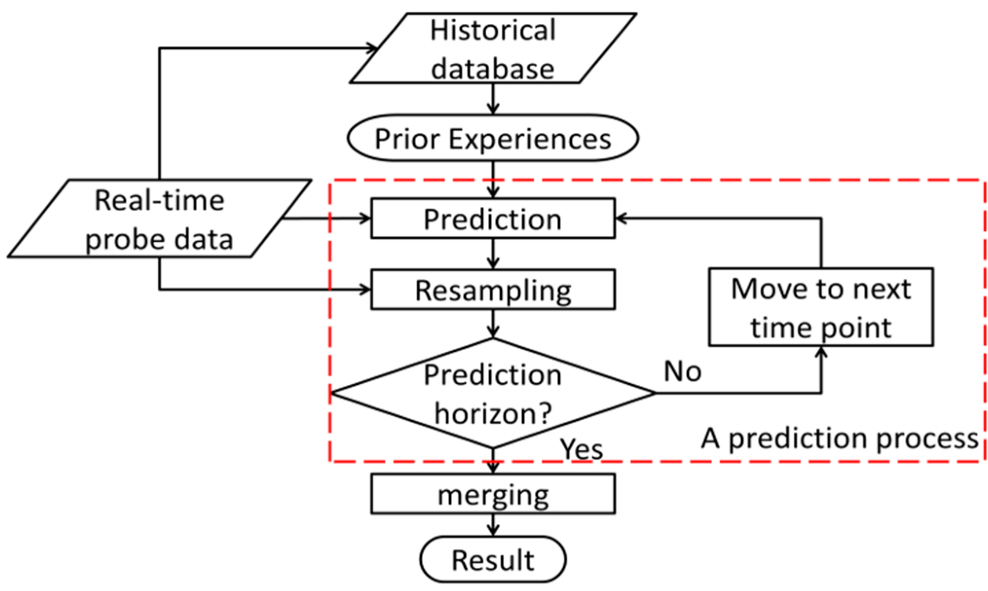
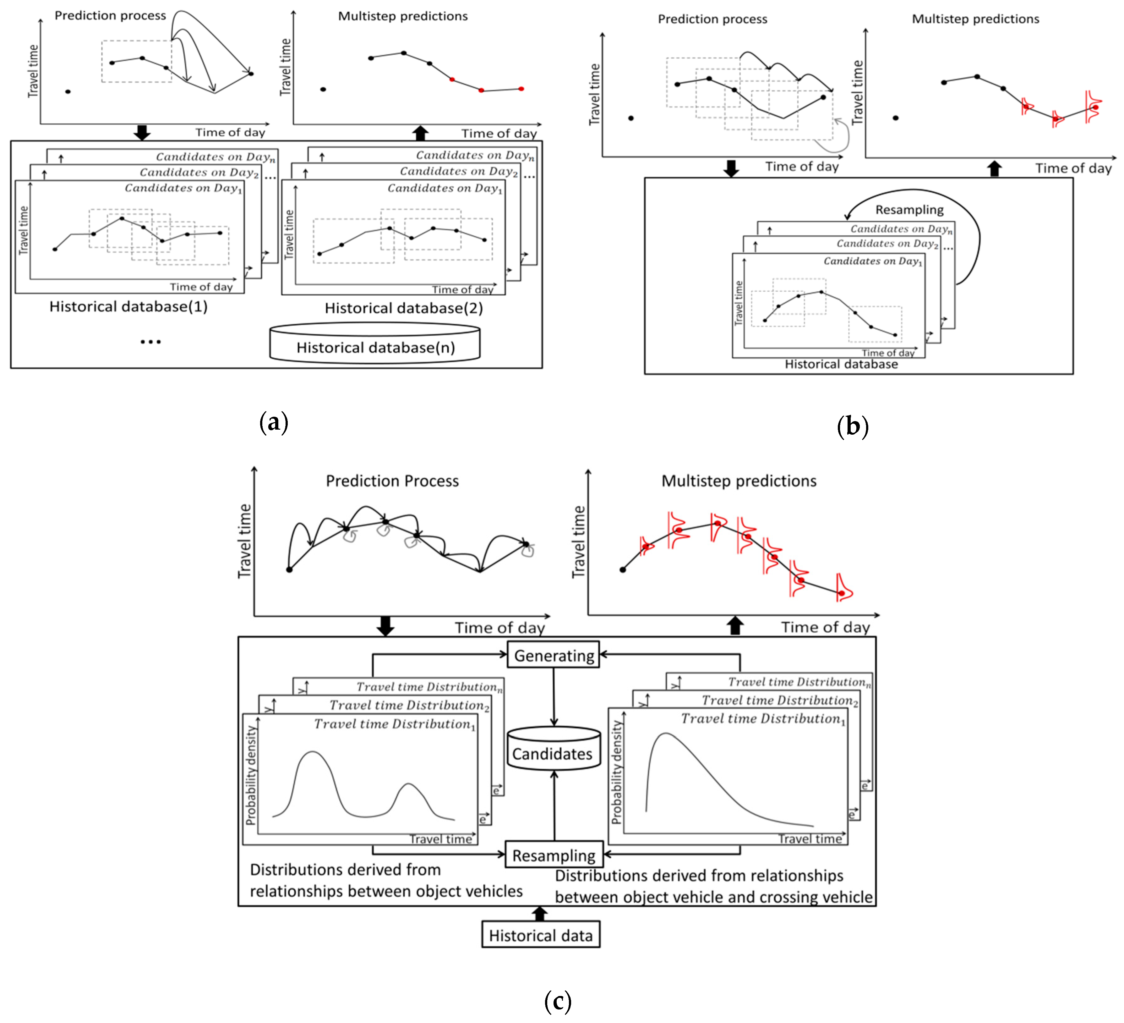
3.1. Descriptions of the Proposed Model
3.2. Details of the Proposed Model
| Algorithm 1. Proposed Travel Time Prediction Process. | |
| 1: | Initialize prediction horizon using Algorithm 3 |
| 2: | If at time point n, there is an observed travel time then |
| 3: | For i = 1:100 do |
| 4: | Generate possible candidate using with error term ; |
| 5: | Calculate similarity for each candidate using (3); |
| 6: | End For |
| 7: | For l = 1: do |
| 8: | For i = 1:100 do |
| 9: | For each possible travel time , calculate probability |
| 10: | at time point (n + l) using (1); |
| 11: | Calculate travel time candidate using (2); |
| 12: | End For |
| 13: | If object vehicle is observed at time point (n + l) then |
| 14: | ; |
| 15: | Begin the resampling process to modify the candidates. |
| 16: | Else if a crossing vehicle is observed at time point (n + l) then |
| 17: | If there is an observed crossing vehicle at time point (n + l − p) then |
| 18: | (l-p < , p < l); |
| 19: | Else |
| 20: | ; |
| 21: | End If |
| 22: | ; |
| 23: | Else, ; |
| 24: | End If |
| 25: | End For |
| 26: | End If |
| Algorithm 2 Resampling. | |
| 1: | If at time point m, an object vehicle data is observed then |
| 2: | Sort candidates according to their weight in decreasing order, |
| 3: | and remove the later 50 candidates; |
| 4: | If at time point m then |
| 5: | For j = 1:100 do |
| 6: | Select according to , calculate weight using (3); |
| 7: | If then |
| 8: | (k = 1…K); |
| 9: | End If |
| 10: | End For |
| 11: | Combine with |
| 12: | and sort candidates according to weight in decreasing order; |
| 13: | Else K = 0; |
| 14: | End If |
| 15: | If 50 + K > 100 then |
| 16: | Remove the later (K − 50) candidates; |
| 17: | End If |
| 18: | If 50 + K < 100 then |
| 19: | Select (50−K) candidates randomly from |
| 20: | according to their weight and add them to ; |
| 21: | End If |
| 22: | End If |
4. Data Process
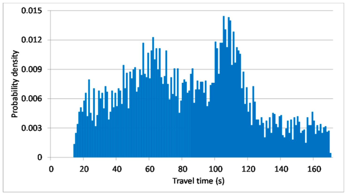
4.1. Data Descriptions
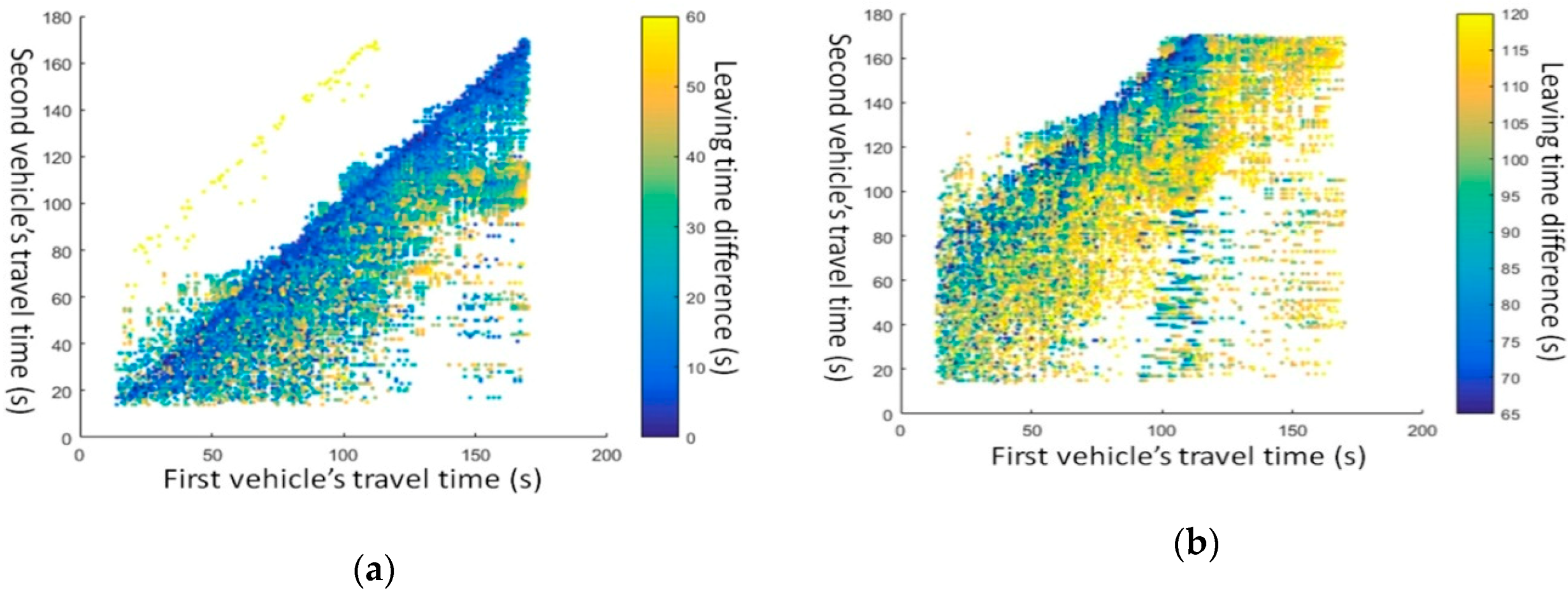
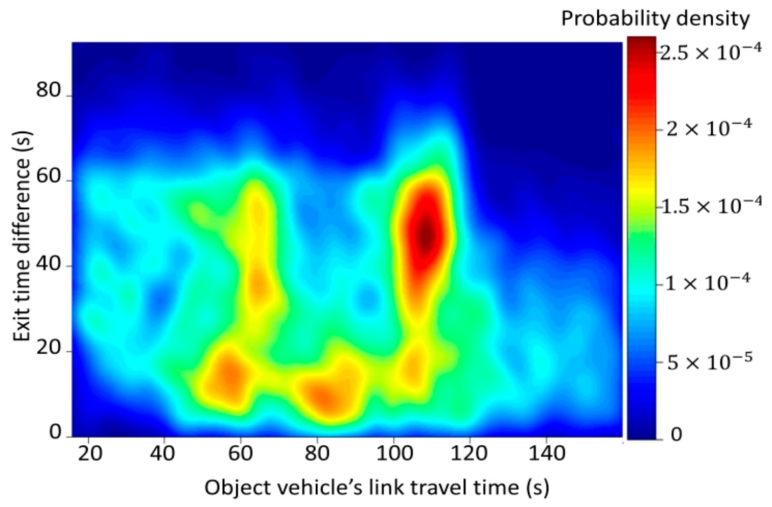
4.2. Relationships between Individual Vehicles
5. Experiments
5.1. Models for Comparison
5.2. Experiment Settings
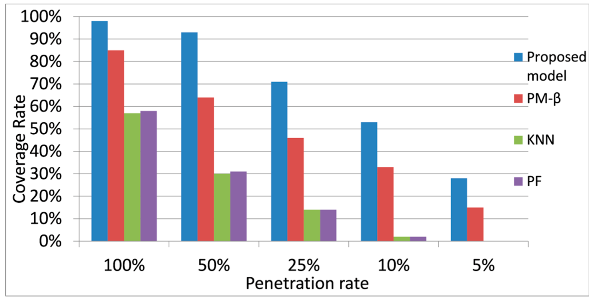
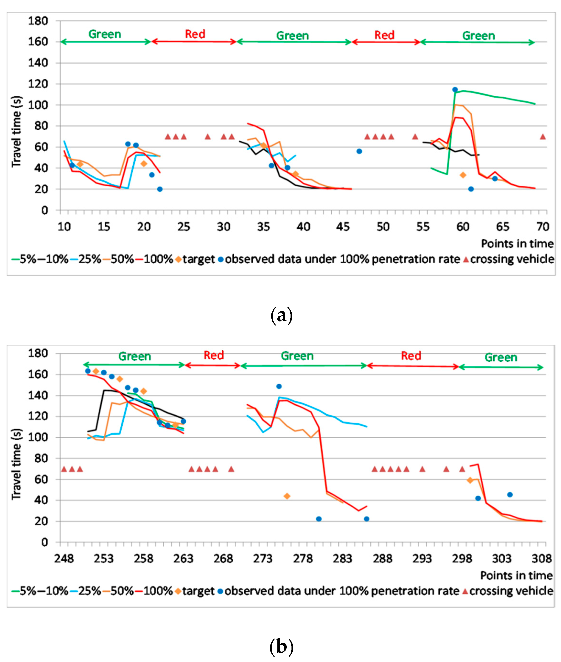
5.3. Results and Discussion
6. Conclusions and Future Work
Author Contributions
Funding
Conflicts of Interest
Appendix A
| Algorithm 3: Signal timing estimation | |
| 1: | For continuous data streams consists of object vehicle data and crossing vehicle data do |
| 2: | If the object vehicle data appear continuously during a period then |
| 3: | Record this period as the green phase |
| 4: | Intervals between each green phase are recorded as the red phase |
| 5: | This record is denoted as {S1} |
| 6: | End If |
| 7: | For all red phases in {S1} do |
| 8: | If the length of a red phase is shorter than 40s then |
| 9: | Change this red phase into the green phase |
| 10: | End If |
| 11: | End For |
| 12: | Remove the first and last phases in {S1} |
| 13: | If the crossing vehicle data appear continuously during a period then |
| 14: | Record this period as a the red phase |
| 15: | Intervals between each red phase are recorded as the green phase |
| 16: | This record is denoted as {S2} |
| 17: | End If |
| 18: | For all green phases in {S2} do |
| 19: | If the length of a green phase is shorter than 40s then |
| 20: | Change this green phase into the red phase |
| 21: | End If |
| 22: | End For |
| 23: | Remove the first and last phases in {S2} |
| 24: | For all red phases in {S2} do |
| 25: | If the length of a red phase is longer than 80 s then |
| 26: | Replace this red phase in {S2} with the corresponding phase in {S1} |
| 27: | End If |
| 28: | End For |
| 29: | Return samples of the green phase and the red phase in {S2} |
| 30: | End For |
| 31: | Calculate and with samples of the green phase between 40 s and 80 s long |
| 32: | Calculate the length of the green phase by A(1) and A(2). |
| 33: | Calculate and with samples of the red phase between 40 s and 80 s long |
| 34: | Calculate the length of the red phase by A(3) and A(4). |
References
- Smith, B.L.; Williams, B.M.; Oswald, R.K. Comparison of parametric and nonparametric models for traffic flow forecasting. Transp. Res. Part C 2002, 10, 303–321. [Google Scholar] [CrossRef]
- Vlahogianni, E.I.; Karlaftis, M.G.; Golias, J.C. Short-term traffic forecasting: Where we are and where we’re going. Transp. Res. Part C 2014, 43, 3–19. [Google Scholar] [CrossRef]
- Shi, C.; Chen, B.Y.; Li, Q. Estimation of travel time distributions in urban road networks using low-frequency floating Car data. ISPRS Int. J. Geo-Inf. 2017, 6, 253. [Google Scholar] [CrossRef]
- Elhenawy, M.; Chen, H.; Rakha, H.A. Dynamic travel time prediction using data clustering and genetic programming. Transp. Res. Part C 2014, 42, 82–98. [Google Scholar] [CrossRef]
- Bucknell, C.; Herrera, J.C. A trade-off analysis between penetration rate and sampling frequency of mobile sensors in traffic state estimation. Transp. Res. Part C 2014, 46, 132–150. [Google Scholar] [CrossRef]
- Lu, L.; Li, X.; Zheng, P.; Wang, K. Determing the required probe vehicle size for real-time travel time estimation on signalized arterial. IEEE Access 2018, 7, 4546–4554. [Google Scholar]
- Chen, H.; Rakha, H.A. Real-time travel time prediction using particle filtering with a non-explicit state-transition model. Transp. Res. Part C 2014, 43, 112–126. [Google Scholar] [CrossRef]
- Guo, J.; Huang, W.; Williams, B.M. Adaptive Kalman filter approach for stochastic short-term traffic flow rate prediction and uncertainty quantification. Transp. Res. Part C 2014, 43, 50–64. [Google Scholar] [CrossRef]
- Habtemichael, F.G.; Cetin, M. Short-term traffic flow rate forecasting based on identifying similar traffic patterns. Transp. Res. Part C 2016, 66, 61–78. [Google Scholar] [CrossRef]
- Argote-Cabañero, J.; Christofa, E.; Skabardonis, A. Connected vehicle penetration rate for estimation of arterial measures of effectiveness. Transp. Res. Part C 2015, 60, 298–312. [Google Scholar] [CrossRef]
- Alrukaibi, F.; Alsaleh, R.; Sayed, T. Real-time travel time estimation in partial network coverage: Case study from Kuwait City. Adv. Transp. Stud. 2018, 44, 79–94. [Google Scholar]
- Bellavista, P.; Caselli, F.; Corradi, A.; Foschini, L. Cooperative Vehicular Traffic Monitoring in Realistic Low Penetration Scenarios: The COLOMBO Experience. Sensors 2018, 18, 822. [Google Scholar] [CrossRef] [PubMed]
- Cheu, R.L.; Xie, C.; Lee, D. Probe Vehicles population and Sample Size for arterial speed Estimation. Comput. Aided Civ. Infrastruct. Eng. 2002, 17, 53–60. [Google Scholar] [CrossRef]
- Jenelius, E.; Koutsopoulos, H.N. Travel time estimation for urban road networks using low frequency probe vehicle data. Transp. Res. Part B 2013, 53, 64–81. [Google Scholar] [CrossRef]
- Sanaullah, I.; Quddus, M.; Enoch, M. Developing travel time estimation methods using sparse GPS data. J. Intell. Transp. Syst. 2016, 20, 532–544. [Google Scholar] [CrossRef]
- Srinivasan, K.K.; Jovanis, P.P. Determination of number of probe vehicles required for reliable travel time measurement in urban networks. Transport. Res. Rec. J. Transport. Res. Board 1996, 1537, 15–22. [Google Scholar] [CrossRef]
- Wan, N.; Vahidi, A.; Luckow, A. Reconstructing maximum likelihood trajectory of probe vehicles between sparse updates. Transp. Res. Part C 2016, 65, 16–30. [Google Scholar] [CrossRef]
- Zheng, F.; Zuylen, H.V. Urban link travel time estimation based on sparse probe vehicle data. Transp. Res. Part C 2013, 31, 145–157. [Google Scholar] [CrossRef]
- Li, Z.; Kluger, R.; Hu, X.; Wu, Y.; Zhu, X. Reconstructing vehicle trajectories to support travel time estimation. Transport. Res. Rec. J. Transp. Res. Board 2018, 2672, 148–158. [Google Scholar] [CrossRef]
- Mori, U.; Mendiburu, A.; Álvarez, M.; Lozano, J.A. A review of travel time estimation and forecasting for advanced traveller information systems. Transp. A Transp. Sci. 2015, 11, 119–157. [Google Scholar] [CrossRef]
- Cai, P.; Wang, Y.; Lu, G.; Chen, P.; Ding, C.; Sun, J. A spatiotemporal correlative k-nearest neighbor model for short-term traffic multistep forecasting. Transp. Res. Part C 2016, 62, 21–34. [Google Scholar] [CrossRef]
- Fusco, G.; Colombaroni, C.; Isaenko, N. Short-term speed predictions exploiting big data on large urban road networks. Transp. Res. Part C 2016, 73, 183–201. [Google Scholar] [CrossRef]
- Habtemichael, F.G.; Cetin, M.; Anuar, K.A. Methodology for quantifying incident-induced delays on freeways by grouping similar traffic patterns. In Proceedings of the 94th Annual Meeting of the Transportation Research Board, Washington, DC, USA, 11–15 January 2015. [Google Scholar]
- Dhivyabharathi, B.; Hima, E.S.; Vanajakshi, L. Stream travel time prediction using particle filtering approach. Transp. Lett. 2016, 1–8. [Google Scholar] [CrossRef]
- Bauer, D.; Tulic, M.; Scherrer, W. Modelling travel time uncertainty in urban networks based on floating taxi data. Eur. Transp. Res. Rev. 2019, 11, 46. [Google Scholar] [CrossRef]
- Wang, J.; Tsapakis, I.; Zhong, C. A space-time delay neural network model for travel time prediction. Eng. Appl. Artif. Intell. 2016, 52, 145–160. [Google Scholar] [CrossRef]
- Petersen, N.C.; Rodrigues, F.; Pereira, F.C. Multi-output bus travel time prediction with convolutional LSTM neural network. Expert Syst. Appl. 2019, 120, 426–435. [Google Scholar] [CrossRef]
- Jenelius, E.; Koutsopoulos, H.N. Urban network travel time prediction based on a probabilistic principal component analysis model of probe data. IEEE Trans. Intell. Transp. Syst. 2018, 19, 436–445. [Google Scholar] [CrossRef]
- Feng, Y.; Hourdos, J.; Davis, G.A. Probe vehicle based real-time traffic monitoring on urban roadways. Transp. Res. Part C 2014, 40, 160–178. [Google Scholar] [CrossRef]
- Carrion, C.; Levinson, D. Value of travel time reliability: A review of current evidence. Transp. Res. Part A 2012, 46, 720–741. [Google Scholar] [CrossRef]
- Li, Z.; Hensher, D.A.; Rose, J.M. Willingness to pay for travel time reliability in passenger transport: A review and some new empirical evidence. Transp. Res. Part E 2010, 46, 384–403. [Google Scholar] [CrossRef]
- Chen, B.Y.; Shi, C.; Zhang, J.; Lam, W.H.K.; Li, Q.; Xiang, S. Most reliable path-finding algorithm for maximizing on-time arrival probability. Transp. B Transp. Dyn. 2016, 5, 248–264. [Google Scholar] [CrossRef]
- Axer, S.; Friedrich, B. Signal timing estimation based on low frequency floating car data. Transp. Res. Procedia 2017, 25, 1648–1664. [Google Scholar] [CrossRef]
- Fayazi, S.A.; Vahidi, A.; Mahler, G.; Winckler, A. Traffic signal phase and timing estimation from low-frequency transit bus data. IEEE Trans. Intell. Transp. Syst. 2015, 16, 19–28. [Google Scholar] [CrossRef]
- Kerper, M.; Wewetzer, C.; Sasse, A.; Mauve, M. Learning traffic light phase schedules from velocity profiles in the cloud. In Proceedings of the 5th International Conference on New Technologies, Mobility and Security (NTMS), Istanbul, Turkey, 7–10 May 2012; pp. 1–5. [Google Scholar]
- Yu, J.; Lu, P. Learning traffic signal phase and timing information from low-sampling rate taxi GPS trajectories. Knowl. Based Syst. 2016, 110, 275–292. [Google Scholar] [CrossRef]
- Fellendorf, M.; Vortisch, P. Validation of the microscopic traffic flow model VISSIM in different real-world situations. In Proceedings of the 80th Annual Meeting of the Transportation Research Board, Washington, DC, USA, 7–11 January 2001. [Google Scholar]
- Bloomberg, L.; Dale, J. A comparison of the VISSIM and CORSIM traffic simulation models. In Proceedings of the Institute of Transportation Engineers Annual Meeting, Nashville, TN, USA, 6–9 August 2000. [Google Scholar]
- Robinson, S.; Polak, J. Modelling urban link travel time with inductive loop detector data by using the k-NN method. Transp. Res. Rec. 2005, 1935, 47–56. [Google Scholar] [CrossRef]


| Term | Definition |
|---|---|
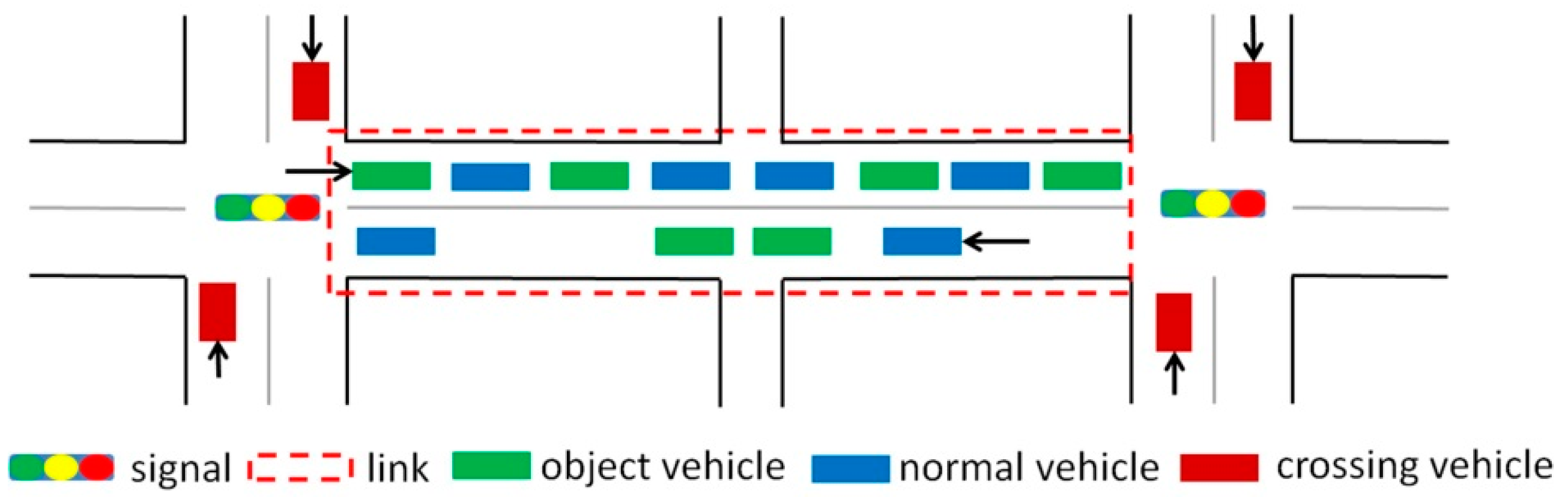
| Object vehicle | Probe vehicle that travels straight through the downstream signalized intersection |
| Normal vehicle | Vehicle that cannot send probe data |
| Crossing vehicle | Probe vehicle traveling in the crossing direction that goes through the same downstream signalized intersection |
| Penetration rate | The ratio of probe vehicles to all vehicles |
| Coverage rate | The proportion of travel time that can be predicted |
| Penetration Rate (%) | 100 | 50 | 25 | 10 | 5 |
|---|---|---|---|---|---|
| Proposed model MAPE (%) | 19.3 | 25.6 | 26.2 | 26.5 | 33.8 |
| Proposed model RMSE | 19.7 | 24.4 | 29.2 | 27.3 | 30.7 |
| Average value MAPE (%) | 71.9 | 65.5 | 57.5 | 58.9 | 54.0 |
| Average value RMSE | 43.1 | 42.6 | 44.3 | 39.8 | 34.2 |
| Penetration Rate (%) | 100 | 50 | 25 | 10 | 5 |
|---|---|---|---|---|---|
| kNN-diff.MAPE (%) | 3.2 | −1.0 | −8.0 | − | − |
| kNN-diff.RMSE | 2.0 | −1.0 | −5.0 | − | − |
| PF-diff.MAPE (%) | −12 | −12 | −27 | − | − |
| PF-diff.RMSE | −9.0 | −9.0 | −15 | − | − |
| PM_-diff.MAPE (%) | 0.0 | 2.0 | 0.0 | −1.0 | −1.0 |
| PM_-diff.RMSE | −3.0 | 1.0 | 2.0 | 0.0 | −6.0 |
© 2020 by the authors. Licensee MDPI, Basel, Switzerland. This article is an open access article distributed under the terms and conditions of the Creative Commons Attribution (CC BY) license (http://creativecommons.org/licenses/by/4.0/).
Share and Cite
Tang, R.; Kanamori, R.; Yamamoto, T. Improving Coverage Rate for Urban Link Travel Time Prediction Using Probe Data in the Low Penetration Rate Environment. Sensors 2020, 20, 265. https://doi.org/10.3390/s20010265
Tang R, Kanamori R, Yamamoto T. Improving Coverage Rate for Urban Link Travel Time Prediction Using Probe Data in the Low Penetration Rate Environment. Sensors. 2020; 20(1):265. https://doi.org/10.3390/s20010265
Chicago/Turabian StyleTang, Ruotian, Ryo Kanamori, and Toshiyuki Yamamoto. 2020. "Improving Coverage Rate for Urban Link Travel Time Prediction Using Probe Data in the Low Penetration Rate Environment" Sensors 20, no. 1: 265. https://doi.org/10.3390/s20010265
APA StyleTang, R., Kanamori, R., & Yamamoto, T. (2020). Improving Coverage Rate for Urban Link Travel Time Prediction Using Probe Data in the Low Penetration Rate Environment. Sensors, 20(1), 265. https://doi.org/10.3390/s20010265