A Robust Multi-Sensor Data Fusion Clustering Algorithm Based on Density Peaks

Abstract
1. Introduction
2. Multi-Sensor Data Fusion
2.1. Multi-Sensor Data Fusion
2.2. Problem Formulation
2.3. CL Constraint and the Size of Clusters
3. Multi-Sensor Data Clustering Algorithm
3.1. Density Peaks Clustering Algorithm
3.2. Target Observations Set and Target Number
3.3. Proposed Clustering Method
| Algorithm 1 Clustering without any overlapping cluster in dataset |
| Input: dataset Z. Output: cluster and its cluster center , . |
| 1.1: Calculate according to (10) and determine whether there is any overlapping cluster in dataset according to (16). If there is no overlapping cluster, go to step 1.2; otherwise, see Algorithm 2. |
| 1.2: Calculate and according to (14) and (15), then cluster using the k-means algorithm. |
| 1.3: Revisit each cluster to make sure that the CL constraint was satisfied, then calculate the cluster center of each cluster. |
| Algorithm 2 Clustering with at least one overlapping cluster in dataset |
| Input: dataset Z. Output: cluster and its cluster center , . |
| 2.1: Calculate according to (11), and we can obtain estimated cluster centers , using the DPC algorithm. |
| 2.2: According to (16), for cluster centers that are , the cluster center is ; for cluster centers that are , calculate and according to (12) and (13), then cluster with the k-means algorithm ( clusters). |
| 2.3: Repeat step 2.2, until all the overlapping clusters are all divided into sub-clusters. |
| 2.4: Revisit each cluster to make sure that the CL constraint was satisfied, then calculate the cluster center of each cluster. |
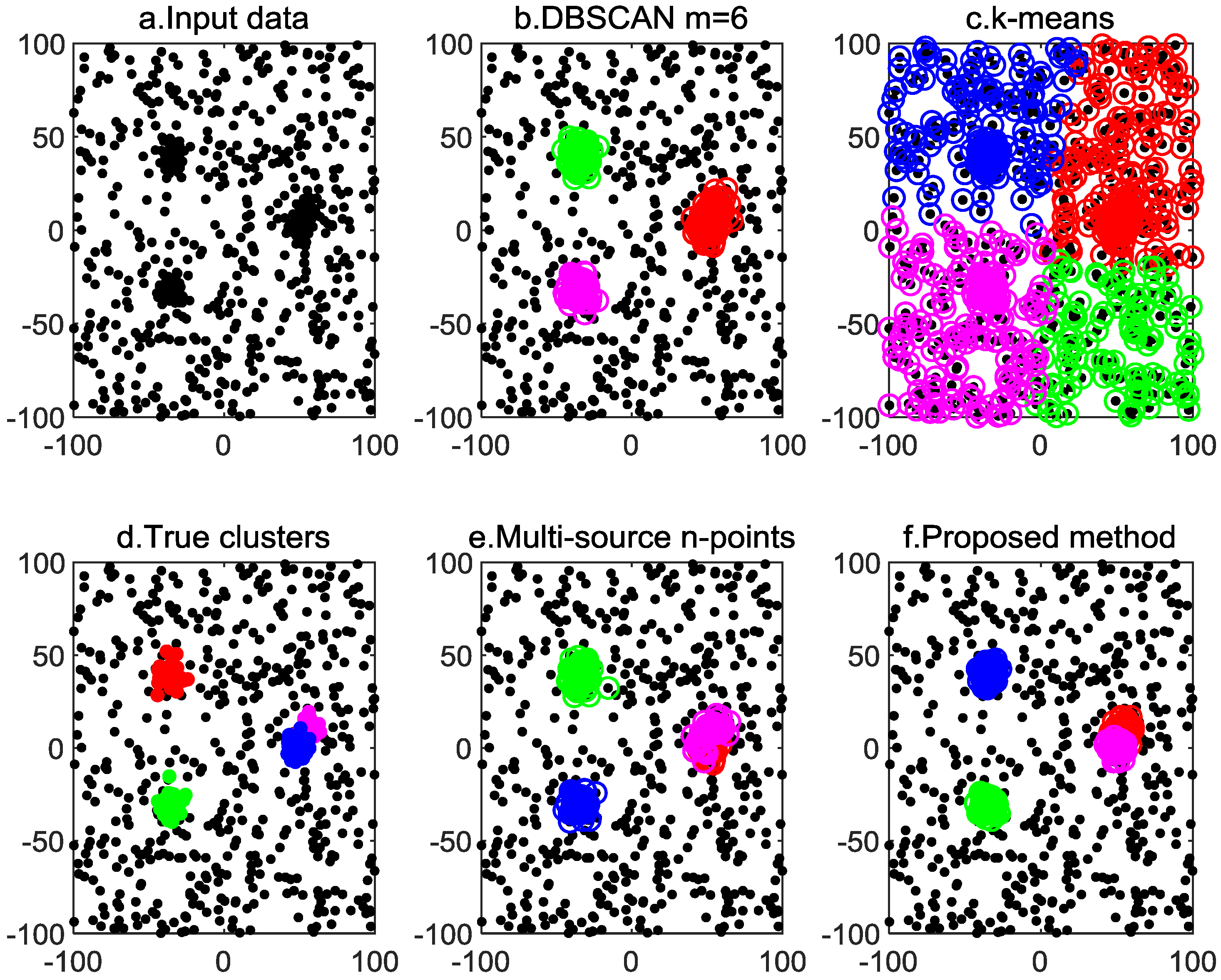
4. Simulation Results
4.1. Given Cutoff Distance
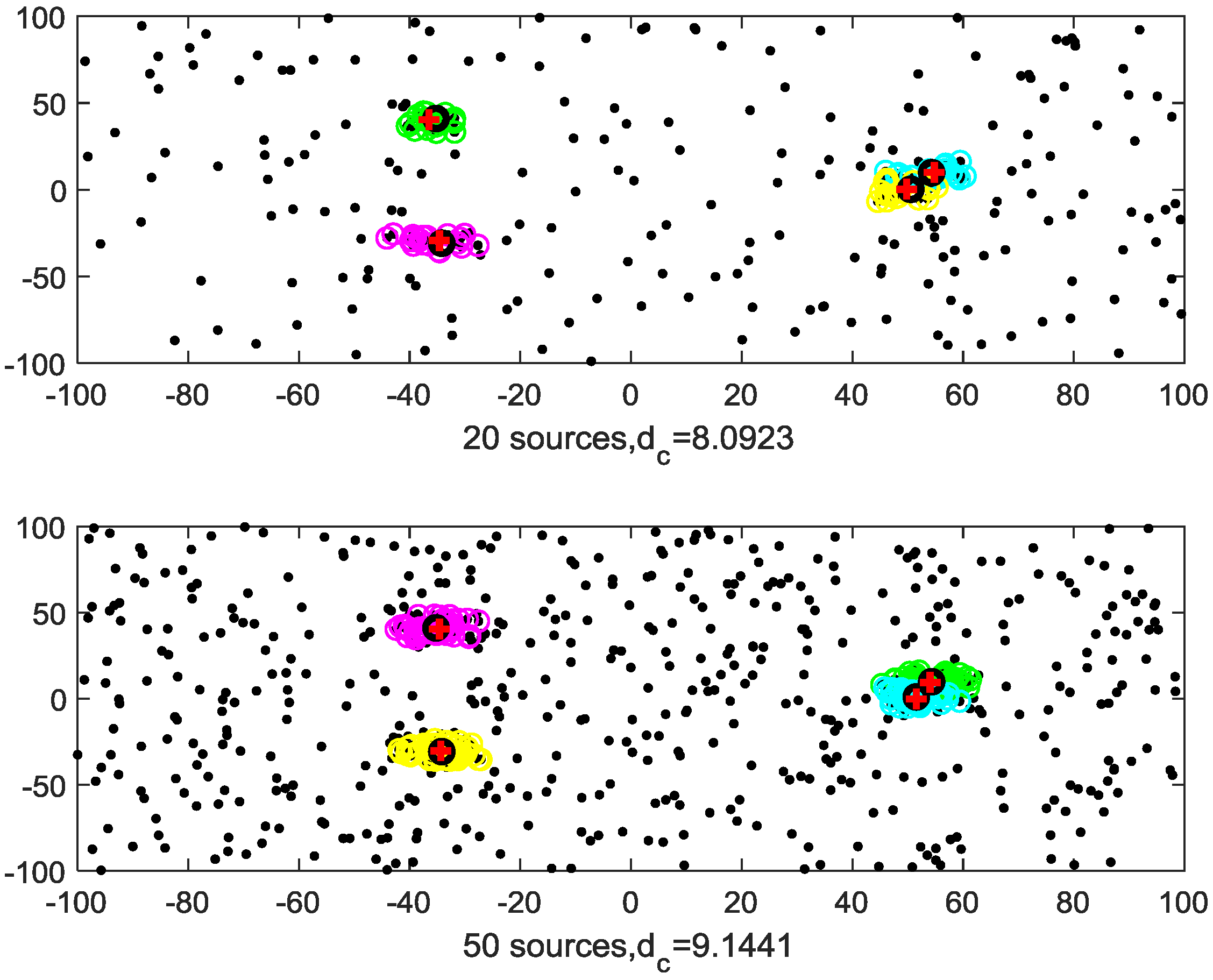
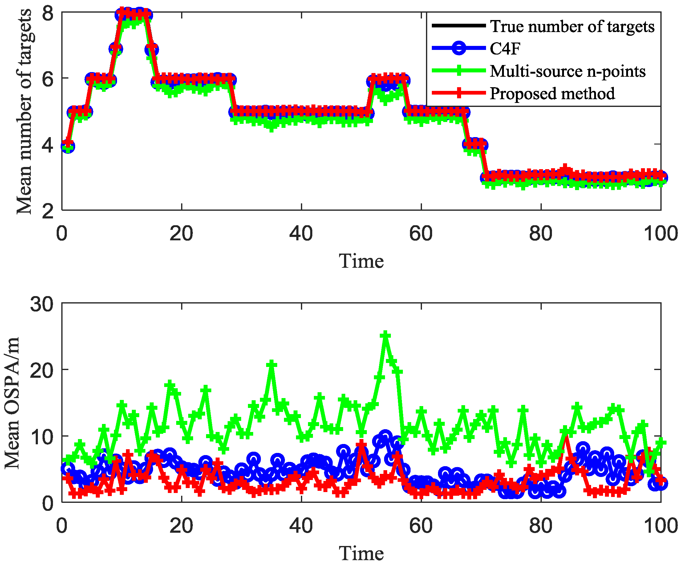
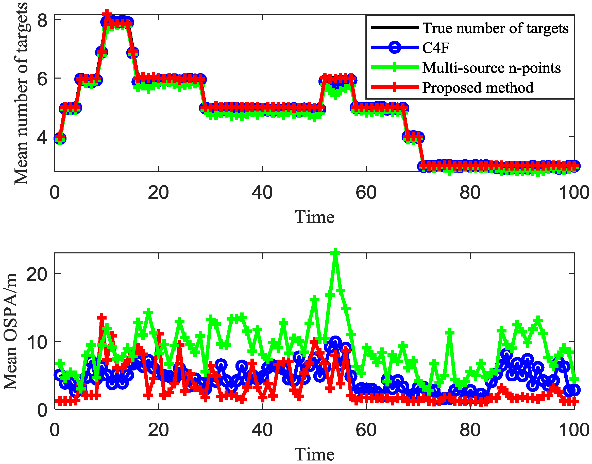
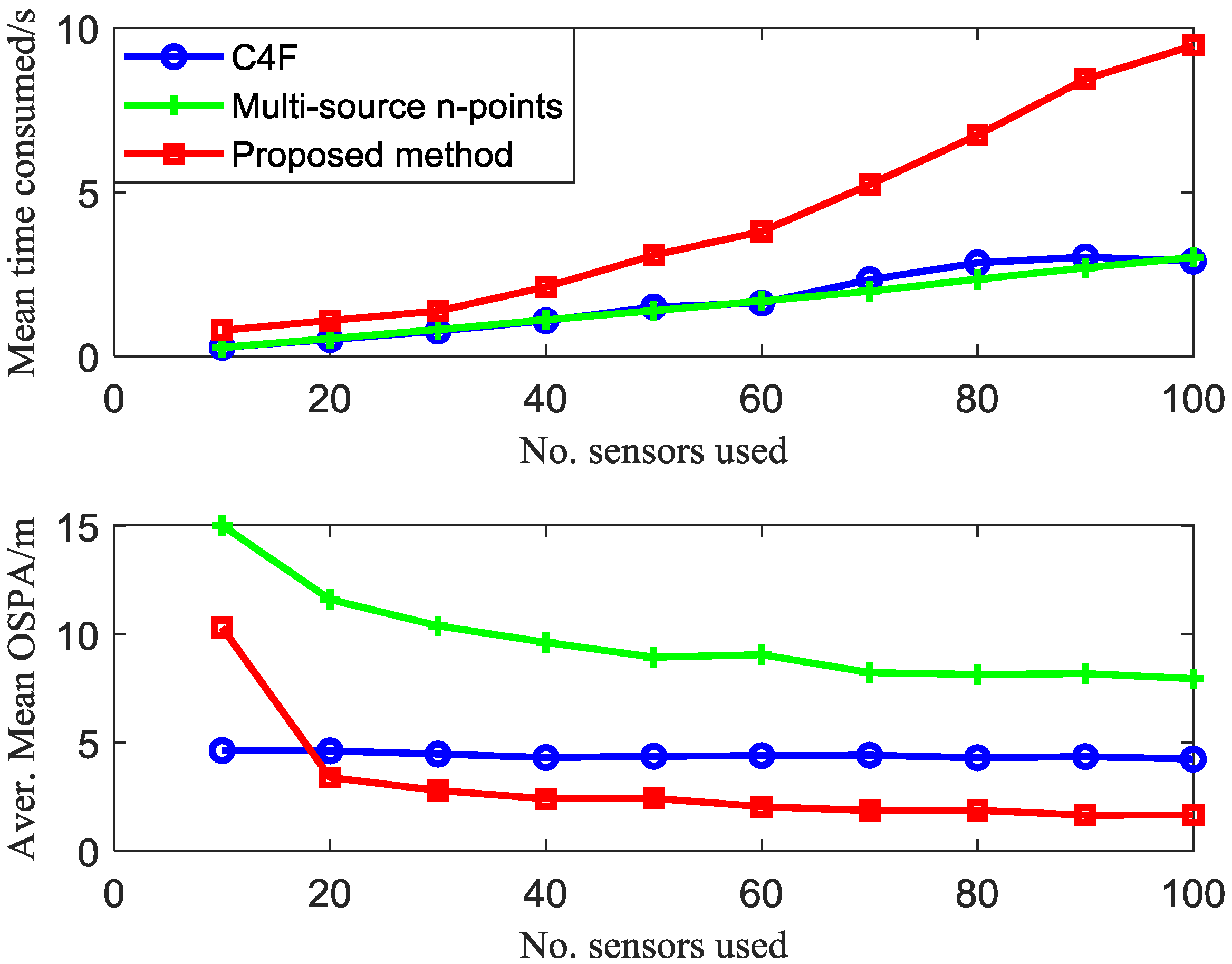
4.2. Unknown Cutoff Distance
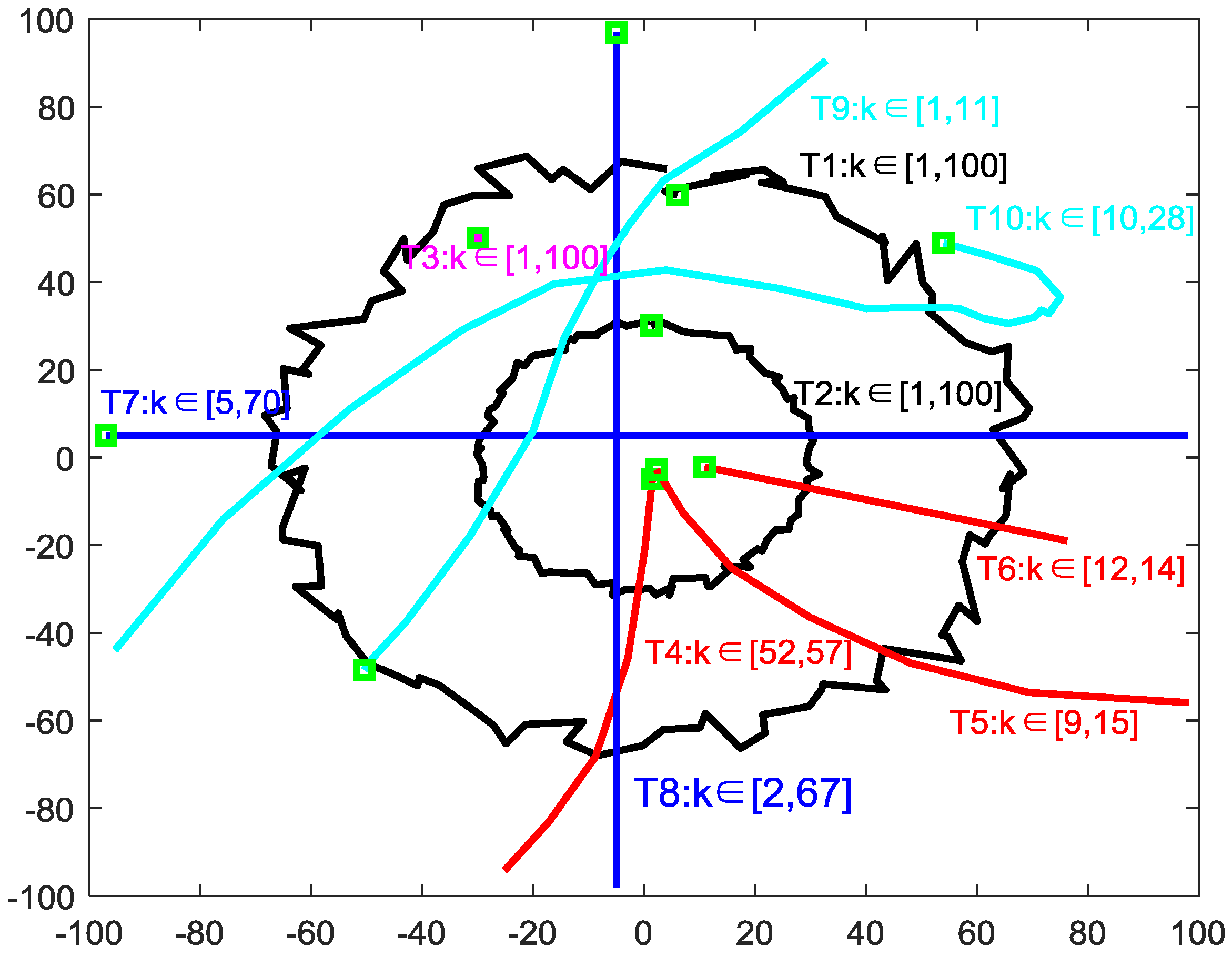
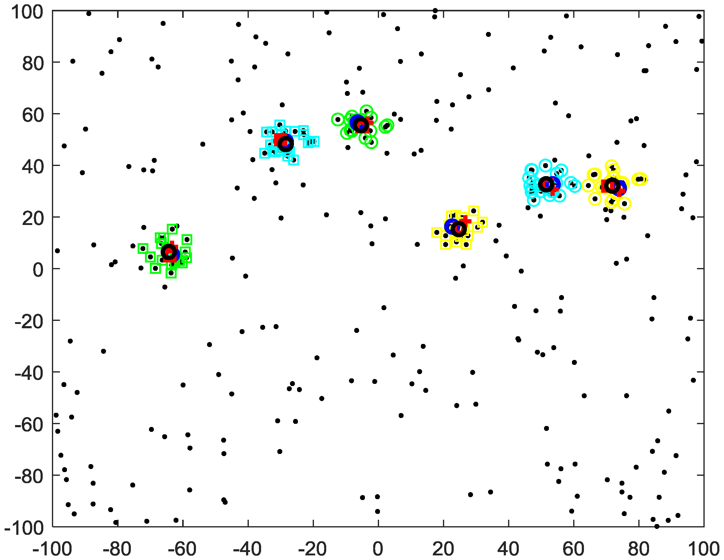
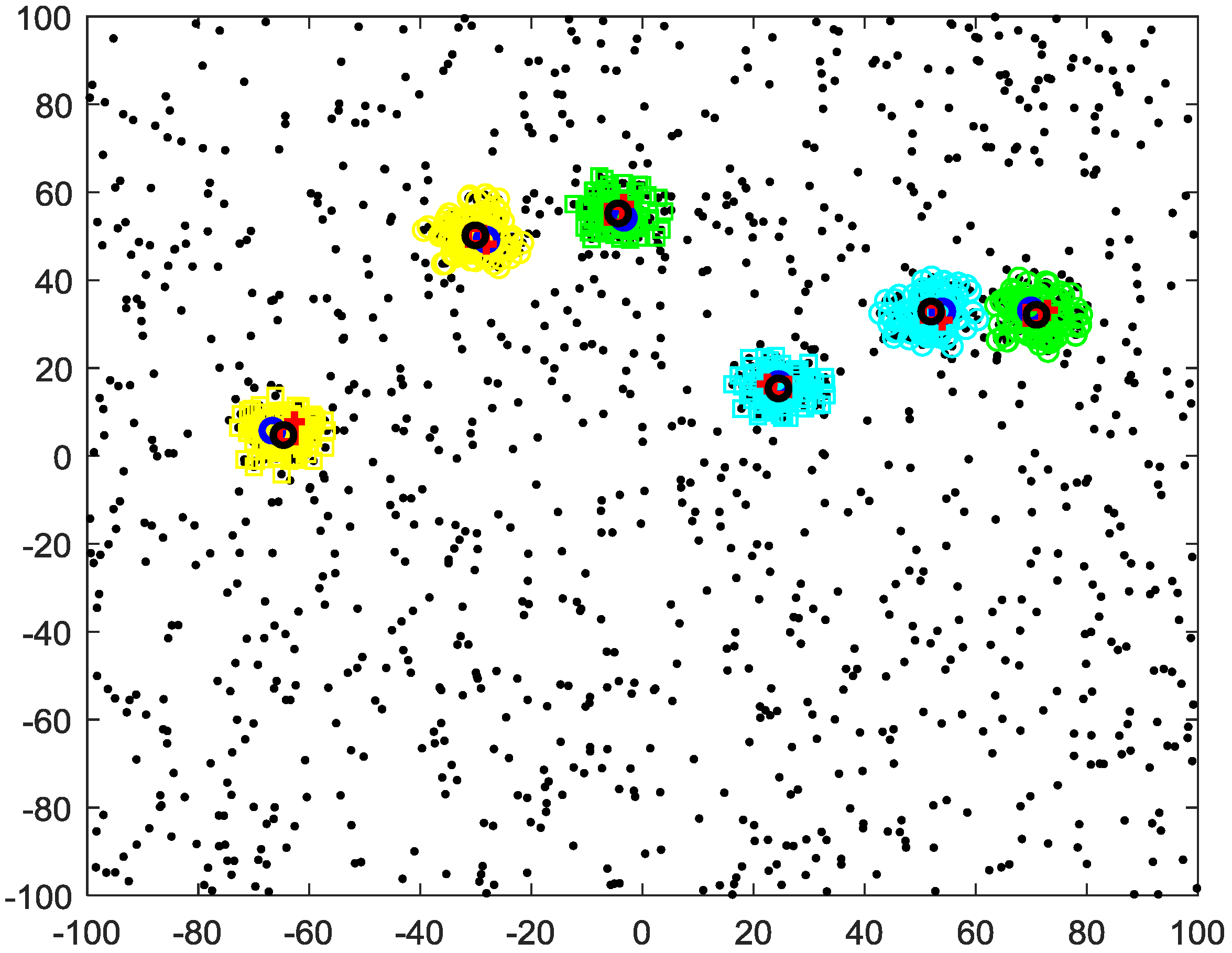
4.3. Clustering-Based Model
5. Conclusions
Author Contributions
Funding
Acknowledgments
Conflicts of Interest
References
- Belkin, M.; Niyogi, P. Laplacian Eigenmaps for dimensionality reduction and data representation. Neural Comput. 2003, 15, 1373–1396. [Google Scholar] [CrossRef]
- Felzenszwalb, P.F.; Huttenlocher, D.P. Efficient graph-based image segmentation. Int. J. Comput. Vis. 2004, 59, 167–181. [Google Scholar] [CrossRef]
- Li, J.; Wang, J.Z. Real-time computerized annotation of pictures. IEEE Trans. Pattern Anal. Mach. Intell. 2008, 30, 985–1002. [Google Scholar] [PubMed]
- Liu, H.; Yu, L. Toward integrating feature selection algorithms for classification and clustering. IEEE Trans. Knowl. Data Eng. 2005, 17, 491–502. [Google Scholar]
- Rodriguez, A.; Laio, A. Clustering by fast search and find of density peaks. Science 2014, 344, 1492–1496. [Google Scholar] [CrossRef]
- Ester, M.; Kriegel, H.; Sander, J. A density-based algorithm for discovering clusters in large spatial Databases with Noise. In Knowledge Discovery and Data Mining; AAAI Press: Palo Alto, CA, USA, 1996; pp. 226–231. [Google Scholar]
- Jain, A.K.; Murty, M.N.; Flynn, P.J. Data clustering: A review. ACM Comput. Surv. 1999, 31, 264–323. [Google Scholar] [CrossRef]
- Wong, J.A.H.A. Algorithm AS 136: A k-means clustering algorithm. J. R. Stat. Soc. Ser. C (Appl. Stat.) 1979, 28, 100–108. [Google Scholar]
- Shi, J.; Malik, J. Normalized cuts and image segmentation. IEEE Trans. Pattern Anal. Mach. Intell. 2000, 22, 888–905. [Google Scholar]
- Navarro, J.F.; Frenk, C.S.; White, S.D. A Universal density profile from hierarchical clustering. Astrophys. J. 1997, 490, 493–508. [Google Scholar] [CrossRef]
- Wagstaff, K.L.; Cardie, C.; Rogers, S. Constrained k-means clustering with background knowledge. In Proceedings of the International Conference on Machine Learning 2001, Williamstown, MA, USA, 28 June–1 July 2001; pp. 577–584. [Google Scholar]
- Han, L.; Luo, S.; Wang, H. An intelligible risk stratification model based on pairwise and size constrained Kmeans. IEEE J. Biomed. Health Inform. 2017, 21, 1288–1296. [Google Scholar] [CrossRef]
- Hansen, P.; Delattre, M. Complete-link cluster analysis by graph coloring. J. Am. Stat. Assoc. 1978, 73, 397–403. [Google Scholar] [CrossRef]
- Miyamoto, S.; Terami, A. Constrained agglomerative hierarchical clustering algorithms with penalties. In Proceedings of the IEEE International Conference on Fuzzy Systems, Taipei, Taiwan, 27–30 June 2011; pp. 422–427. [Google Scholar]
- Goode, A. X-means: Extending k-means with efficient estimation of the number of clusters. In Intelligent Data Engineering and Automated Learning—IDEAL 2000. Data Mining, Financial Engineering, and Intelligent Agents; Springer: Berlin/Heidelberg, Germany, 2000. [Google Scholar]
- Akaike, H.T. A new look at the statistical model identification. IEEE Trans. Autom. Control 1974, 19, 716–723. [Google Scholar] [CrossRef]
- Davisson, L. Rate distortion theory: A mathematical basis for data compression. IEEE Trans. Commun. 2003, 20, 1202. [Google Scholar] [CrossRef]
- Arthur, D.; Vassilvitskii, S. K-Means++: The advantages of careful seeding. In Proceedings of the Eighteenth Annual ACM-SIAM Symposium on Discrete Algorithms, SODA 2007, New Orleans, LA, USA, 7–9 January 2007. [Google Scholar]
- Coue, C.; Fraichard, T.; Bessiere, P. Using Bayesian Programming for multi-sensor multi-target tracking in automotive applications. In Proceedings of the International Conference on Robotics and Automation 2003, Taipei, Taiwan, 14–19 September 2003; pp. 2104–2109. [Google Scholar]
- Qiao, D.; Liang, Y.; Jiao, L. Boundary detection-based density peaks clustering. IEEE Access 2019, 19, 755–765. [Google Scholar] [CrossRef]
- Jiang, J.; Chen, Y.; Meng, X.; Wang, L.; Li, K. A novel density peaks clustering algorithm based on k nearest neighbors for improving assignment process. Phys. A Stat. Mech. Appl. 2019, 523, 702–713. [Google Scholar] [CrossRef]
- Li, T.; Corchado, J.M.; Sun, S. Partial consensus and conservative fusion of Gaussian mixtures for distributed PHD fusion. IEEE Trans. Aerosp. Electron. Syst. 2018, 55, 2150–2163. [Google Scholar] [CrossRef]
- Vo, B.; See, C.M.; Ma, N. Multi-sensor joint detection and tracking with the Bernoulli filter. IEEE Trans. Aerosp. Electron. Syst. 2012, 48, 1385–1402. [Google Scholar] [CrossRef]
- Li, T.; Corchado, J.M.; Sun, S. Clustering for filtering: Multi-object detection and estimation using multiple/massive sensors. Inf. Sci. 2017, 388–389, 172–190. [Google Scholar] [CrossRef]
- Li, T.; Corchado, J.M.; Chen, H. Distributed flooding-then-clustering: A lazy networking approach for distributed multiple target tracking. In Proceedings of the International Conference on Information Fusion 2018, Cambridge, UK, 10–13 July 2018; pp. 2415–2422. [Google Scholar]
- Li, T.; Pintado, F.D.; Corchado, J.M. Multi-source homogeneous data clustering for multi-target detection from cluttered background with misdetection. Appl. Soft Comput. 2017, 60, 436–446. [Google Scholar] [CrossRef]
- Shi, Q.; Zhang, T.; Cui, G.; Kong, L. Multi-target tracking algorithm based on multi-sensor clustering in distributed radar network. Fusion 2019, in press. [Google Scholar]
- Li, T.; Prieto, J.; Fan, H. A robust multi-sensor PHD filter based on multi-sensor measurement clustering. IEEE Commun. Lett. 2018, 22, 2064–2067. [Google Scholar] [CrossRef]
- Schuhmacher, D.; Vo, B.T.; Vo, B.N. A consistent metric for performance evaluation of multi-object filters. IEEE Trans. Signal Process. 2008, 56, 3447–3457. [Google Scholar] [CrossRef]


| Algorithms | k-Means | DBSCAN | Multi-Source n-Points | Proposed Method |
|---|---|---|---|---|
| Parameters | / |
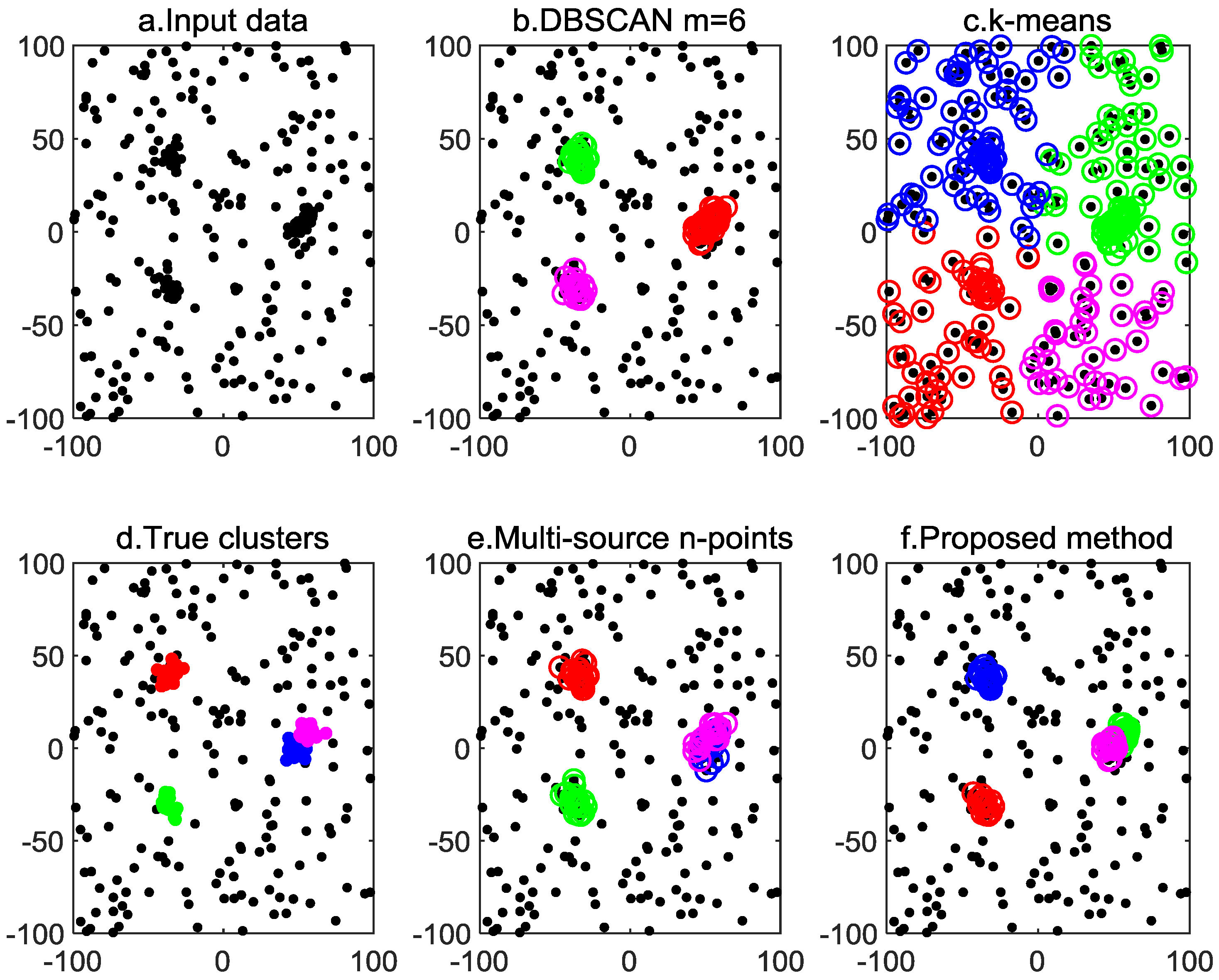
| Algorithms | k-Means | DBSCAN m = 6 | Multi-Source n-Points | Proposed Method |
|---|---|---|---|---|
| Figure 4 | 0.0059 | 0.0021 | 0.0051 | 0.0078 |
| Figure 5 | 0.0087 | 0.0145 | 0.0198 | 0.0346 |
| Algorithms | Multi-Source n-Points | Proposed Method |
|---|---|---|
| 20 sensors | 6.7815 | 8.0932 |
| 50 sensors | 5.9779 | 9.1440 |
© 2019 by the authors. Licensee MDPI, Basel, Switzerland. This article is an open access article distributed under the terms and conditions of the Creative Commons Attribution (CC BY) license (http://creativecommons.org/licenses/by/4.0/).
Share and Cite
Fan, J.; Xie, W.; Du, H. A Robust Multi-Sensor Data Fusion Clustering Algorithm Based on Density Peaks. Sensors 2020, 20, 238. https://doi.org/10.3390/s20010238
Fan J, Xie W, Du H. A Robust Multi-Sensor Data Fusion Clustering Algorithm Based on Density Peaks. Sensors. 2020; 20(1):238. https://doi.org/10.3390/s20010238
Chicago/Turabian StyleFan, Jiande, Weixin Xie, and Haocui Du. 2020. "A Robust Multi-Sensor Data Fusion Clustering Algorithm Based on Density Peaks" Sensors 20, no. 1: 238. https://doi.org/10.3390/s20010238
APA StyleFan, J., Xie, W., & Du, H. (2020). A Robust Multi-Sensor Data Fusion Clustering Algorithm Based on Density Peaks. Sensors, 20(1), 238. https://doi.org/10.3390/s20010238