Influence of Resonances on the Noise Performance of SQUID Susceptometers


Abstract
1. Introduction
2. Modeling
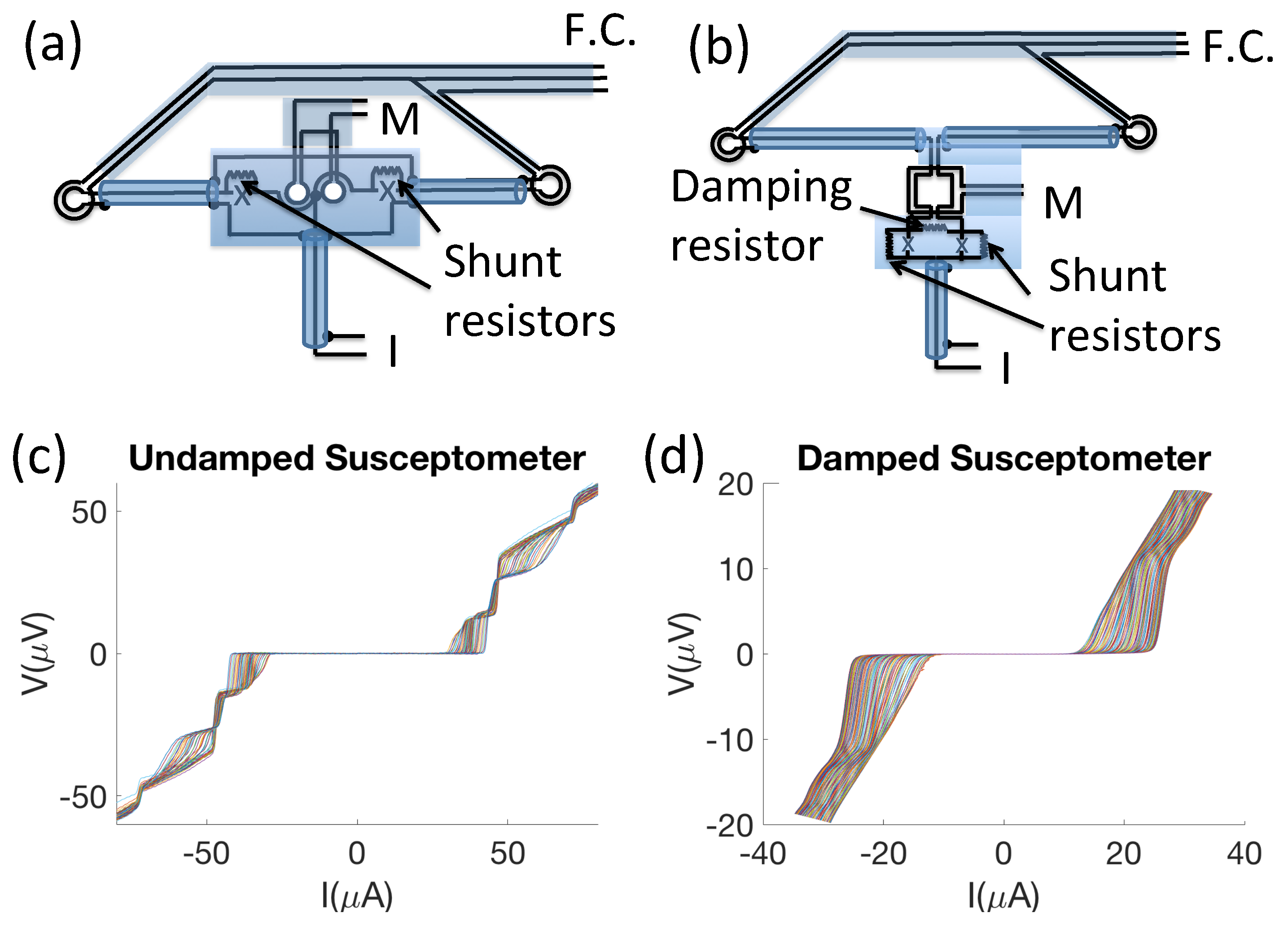
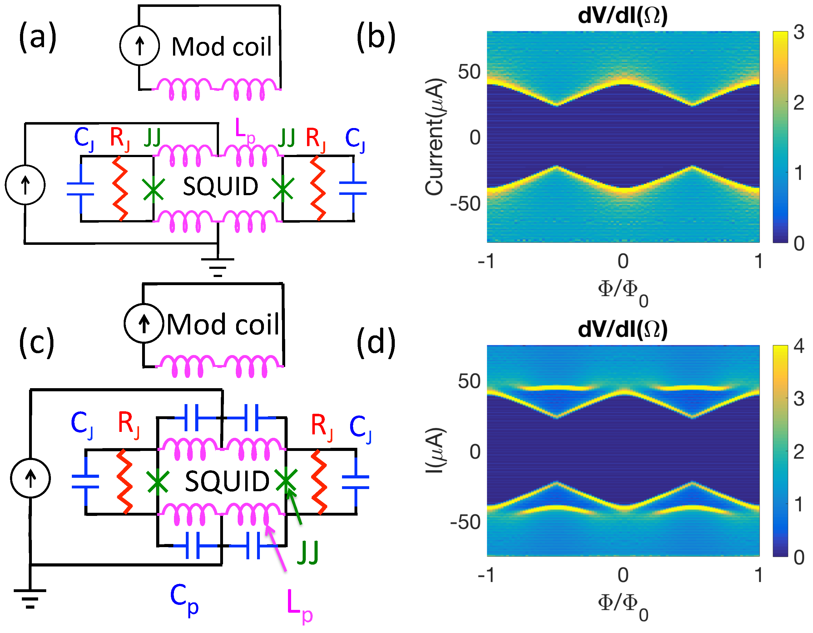
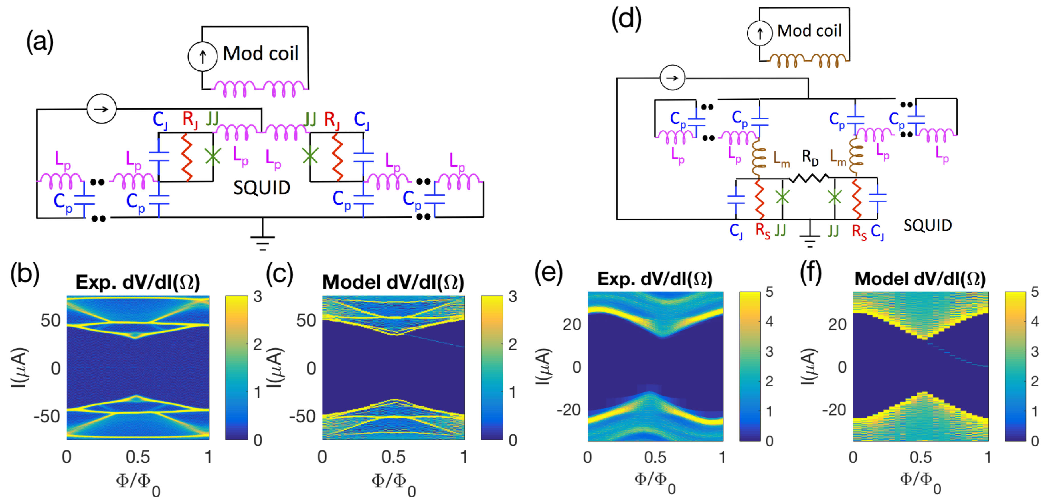
2.1. IR Characteristics
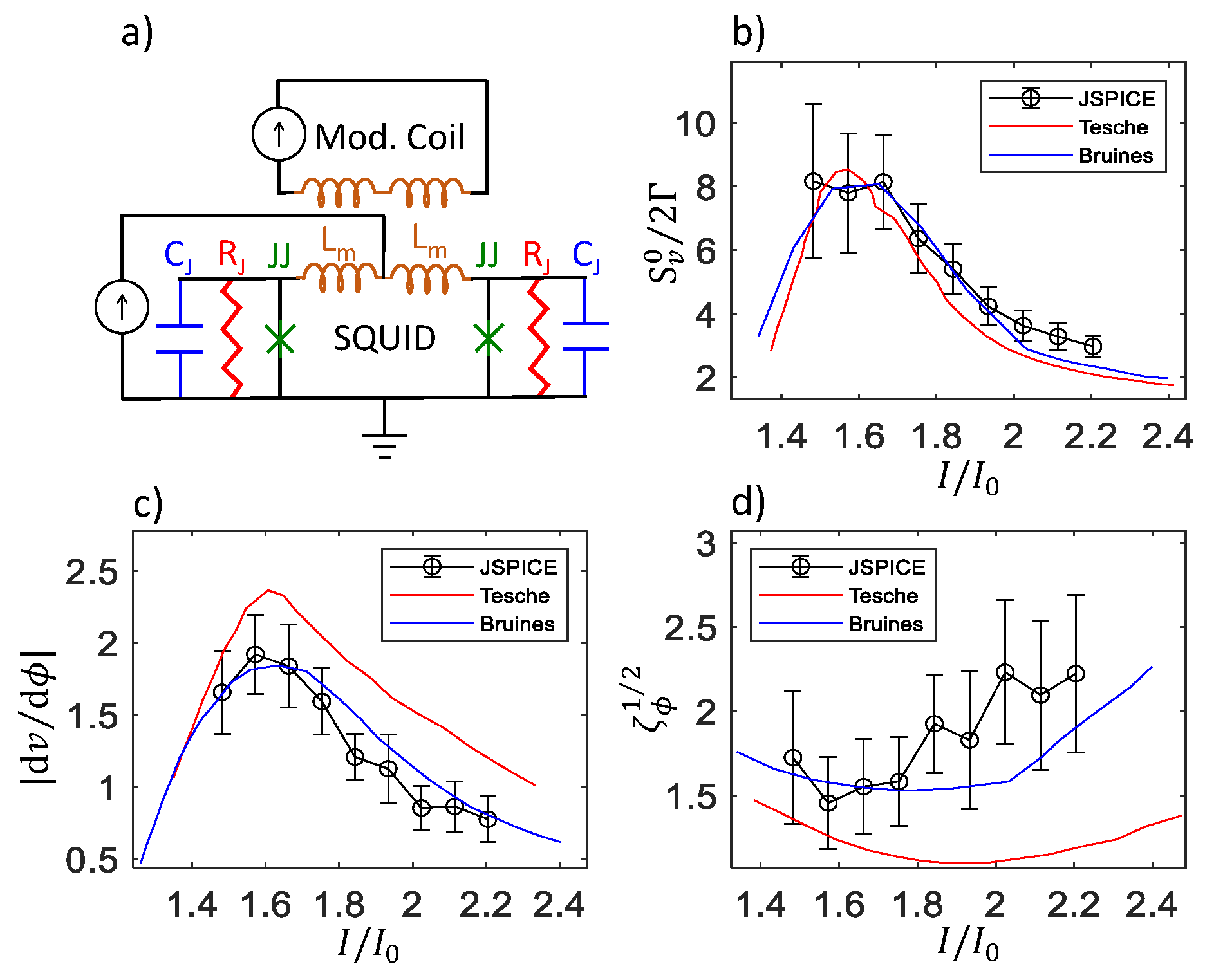
2.2. Noise
2.3. Summary of Noise Calculations
Author Contributions
Funding
Acknowledgments
Conflicts of Interest
References
- Clarke, J.; Braginski, A.I. The SQUID Handbook; Wiley Online Library: Hoboken, NJ, USA, 2004. [Google Scholar]
- Vinante, A.; Mezzena, R.; Prodi, G.A.; Vitale, S.; Cerdonio, M.; Falferi, P.; Bonaldi, M. Dc superconducting quantum interference device amplifier for gravitational wave detectors with a true noise temperature of 16 μK. Appl. Phys. Lett. 2001, 79, 2597–2599. [Google Scholar] [CrossRef]
- Harry, G.M.; Jin, I.; Paik, H.J.; Stevenson, T.R.; Wellstood, F.C. Two-stage superconducting-quantum-interference-device amplifier in a high-Q gravitational wave transducer. Appl. Phys. Lett. 2000, 76, 1446–1448. [Google Scholar] [CrossRef][Green Version]
- Hari, R.; Salmelin, R. Magnetoencephalography: From SQUIDs to neuroscience: Neuroimage 20th anniversary special edition. Neuroimage 2012, 61, 386–396. [Google Scholar] [CrossRef]
- Devoret, M.H.; Wallraff, A.; Martinis, J.M. Superconducting qubits: A short review. arXiv 2004, arXiv:cond-mat/0411174. [Google Scholar]
- Kirtley, J.R.; Wikswo, J.P., Jr. Scanning SQUID microscopy. Annu. Rev. Mater. Sci. 1999, 29, 117–148. [Google Scholar] [CrossRef]
- Black, R.; Mathai, A.; Wellstood, F.; Dantsker, E.; Miklich, A.; Nemeth, D.; Kingston, J.; Clarke, J. Magnetic microscopy using a liquid nitrogen cooled YBa2Cu3O7 superconducting quantum interference device. Appl. Phys. Lett. 1993, 62, 2128–2130. [Google Scholar] [CrossRef]
- Veauvy, C.; Hasselbach, K.; Mailly, D. Scanning μ-superconduction quantum interference device force microscope. Rev. Sci. Instrum. 2002, 73, 3825–3830. [Google Scholar] [CrossRef]
- Finkler, A.; Segev, Y.; Myasoedov, Y.; Rappaport, M.L.; Ne’eman, L.; Vasyukov, D.; Zeldov, E.; Huber, M.E.; Martin, J.; Yacoby, A. Self-aligned nanoscale SQUID on a tip. Nano Lett. 2010, 10, 1046–1049. [Google Scholar] [CrossRef]
- Vu, L.; Wistrom, M.; Van Harlingen, D.J. Imaging of magnetic vortices in superconducting networks and clusters by scanning SQUID microscopy. Appl. Phys. Lett. 1993, 63, 1693–1695. [Google Scholar] [CrossRef]
- Kirtley, J.; Ketchen, M.; Stawiasz, K.; Sun, J.; Gallagher, W.; Blanton, S.; Wind, S. High-resolution scanning SQUID microscope. Appl. Phys. Lett. 1995, 66, 1138–1140. [Google Scholar] [CrossRef]
- Gardner, B.W.; Wynn, J.C.; Björnsson, P.G.; Straver, E.W.; Moler, K.A.; Kirtley, J.R.; Ketchen, M.B. Scanning superconducting quantum interference device susceptometry. Rev. Sci. Instrum. 2001, 72, 2361–2364. [Google Scholar] [CrossRef]
- Kirtley, J. Fundamental studies of superconductors using scanning magnetic imaging. Rep. Prog. Phys. 2010, 73, 126501. [Google Scholar] [CrossRef]
- Huber, M.E.; Koshnick, N.C.; Bluhm, H.; Archuleta, L.J.; Azua, T.; Björnsson, P.G.; Gardner, B.W.; Halloran, S.T.; Lucero, E.A.; Moler, K.A. Gradiometric micro-SQUID susceptometer for scanning measurements of mesoscopic samples. Rev. Sci. Instrum. 2008, 79, 053704. [Google Scholar] [CrossRef] [PubMed]
- Kirtley, J.R.; Paulius, L.; Rosenberg, A.J.; Palmstrom, J.C.; Holland, C.M.; Spanton, E.M.; Schiessl, D.; Jermain, C.L.; Gibbons, J.; Fung, Y.K.K.; et al. Scanning SQUID susceptometers with sub-micron spatial resolution. Rev. Sci. Instrum. 2016, 87, 093702. [Google Scholar] [CrossRef] [PubMed]
- Tesche, C.D.; Clarke, J. dc SQUID: Noise and Optimization. J. Low Temp. Phys. 1977, 29, 301–331. [Google Scholar] [CrossRef]
- Bruines, J.; de Waal, V.; Mooij, J. Comment on: “Dc SQUID: Noise and optimization” by Tesche and Clarke. J. Low Temp. Phys. 1982, 46, 383–386. [Google Scholar] [CrossRef]
- Hilbert, C.; Clarke, J. Measurements of the dynamic input impedance of a dc SQUID. J. Low Temp. Phys. 1985, 61, 237–262. [Google Scholar] [CrossRef]
- Enpuku, K.; Cantor, R.; Koch, H. Modeling the dc superconducting quantum interference device coupled to the multiturn input coil. III. J. Appl. Phys. 1992, 72, 1000–1006. [Google Scholar] [CrossRef]
- Huber, M.E.; Neil, P.A.; Benson, R.G.; Burns, D.A.; Corey, A.; Flynn, C.S.; Kitaygorodskaya, Y.; Massihzadeh, O.; Martinis, J.M.; Hilton, G. DC SQUID series array amplifiers with 120 MHz bandwidth (corrected). IEEE Trans. Appl. Supercond. 2001, 11, 4048–4053. [Google Scholar] [CrossRef]
- Knuutila, J.; Ahonen, A.; Tesche, C. Effects on dc SQUID characteristics of damping of input coil resonances. J. Low Temp. Phys. 1987, 68, 269–284. [Google Scholar] [CrossRef]
- Josephson, B.D. Possible new effects in superconductive tunnelling. Phys. Lett. 1962, 1, 251–253. [Google Scholar] [CrossRef]
- IC Design Software for Linux, OS X and Windows. Available online: http://www.wrcad.com/ (accessed on 13 September 2019).
- JSPICE. Available online: https://ptolemy.berkeley.edu/projects/embedded/pubs/downloads/spice/jspice.html (accessed on 11 March 2019).


| Parameter | Symbol | Conversion Formula |
|---|---|---|
| Voltage | v | |
| Magnetic flux | ||
| Thermal noise parameter | ||
| Voltage noise power | ||
| Flux noise | ||
| Hysteresis parameter |
© 2019 by the authors. Licensee MDPI, Basel, Switzerland. This article is an open access article distributed under the terms and conditions of the Creative Commons Attribution (CC BY) license (http://creativecommons.org/licenses/by/4.0/).
Share and Cite
Davis, S.I.; Kirtley, J.R.; Moler, K.A. Influence of Resonances on the Noise Performance of SQUID Susceptometers. Sensors 2020, 20, 204. https://doi.org/10.3390/s20010204
Davis SI, Kirtley JR, Moler KA. Influence of Resonances on the Noise Performance of SQUID Susceptometers. Sensors. 2020; 20(1):204. https://doi.org/10.3390/s20010204
Chicago/Turabian StyleDavis, Samantha I., John R. Kirtley, and Kathryn A. Moler. 2020. "Influence of Resonances on the Noise Performance of SQUID Susceptometers" Sensors 20, no. 1: 204. https://doi.org/10.3390/s20010204
APA StyleDavis, S. I., Kirtley, J. R., & Moler, K. A. (2020). Influence of Resonances on the Noise Performance of SQUID Susceptometers. Sensors, 20(1), 204. https://doi.org/10.3390/s20010204