SPS and DPS: Two New Grid-Based Source Location Privacy Protection Schemes in Wireless Sensor Networks


Abstract
:1. Introduction
1.1. Related Works and Issues
1.2. Our Motivations and Contributions
1.3. Organization of the Paper
2. System Model
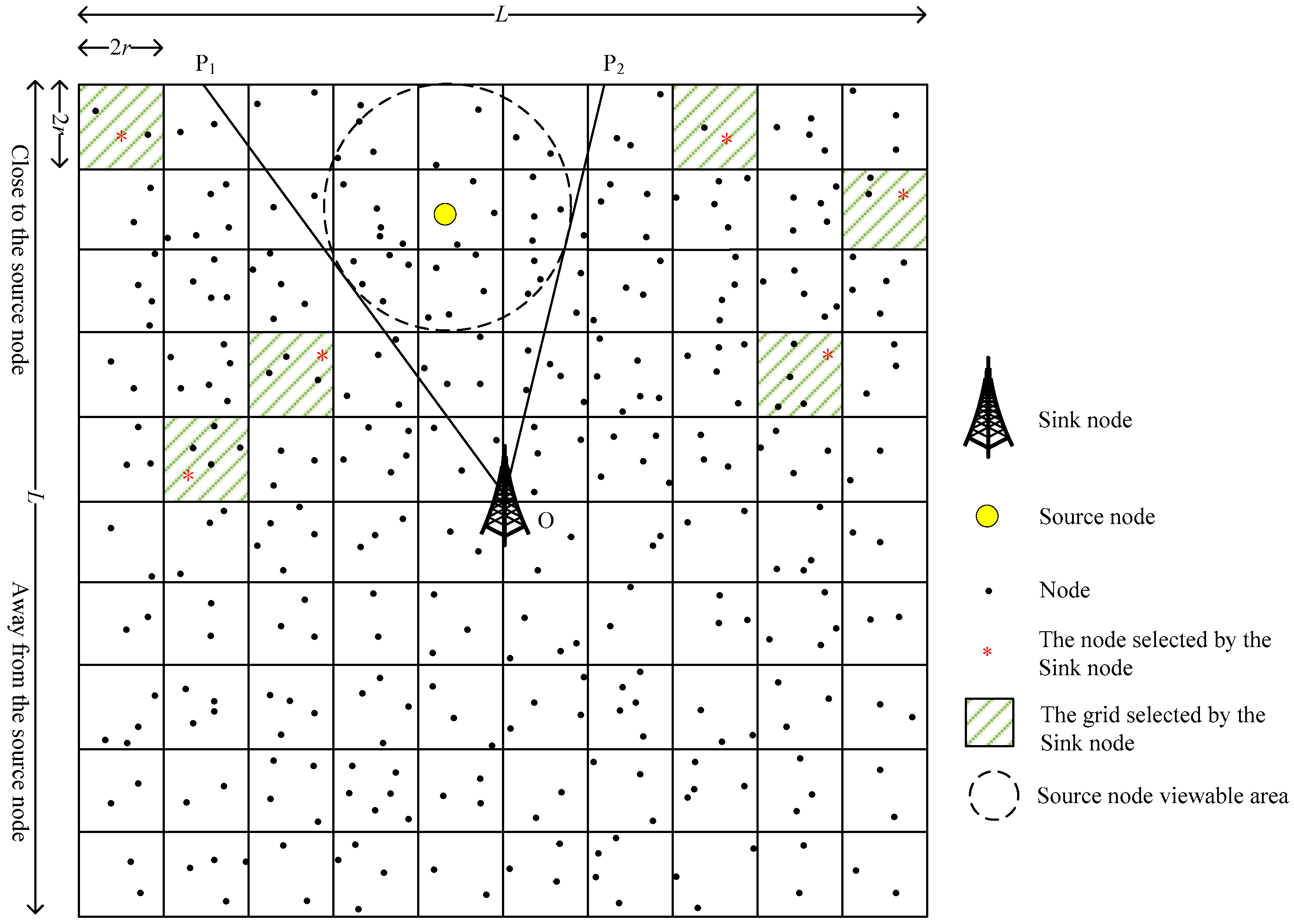
2.1. Network Model
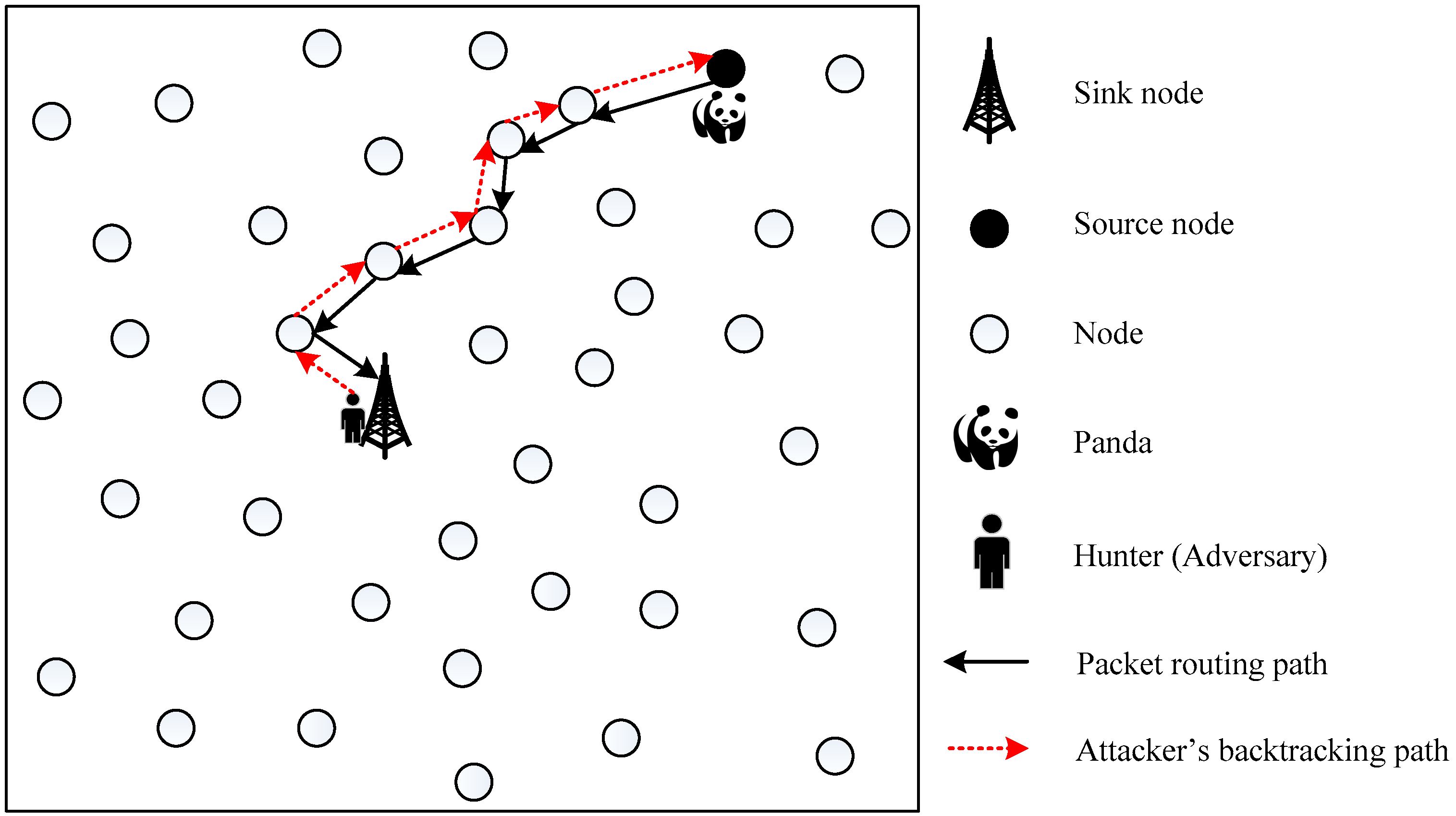
2.2. Attack Model
2.3. Security Model
3. SPS: Grid-Based Single Phantom Node Source Location Privacy Protection Scheme
3.1. The Initialization Phase
- Near-hop neighbor node: ;
- Same-hop neighbor node: ;
- Far-hop neighbor node: .
3.2. The Phantom Node Determination Phase
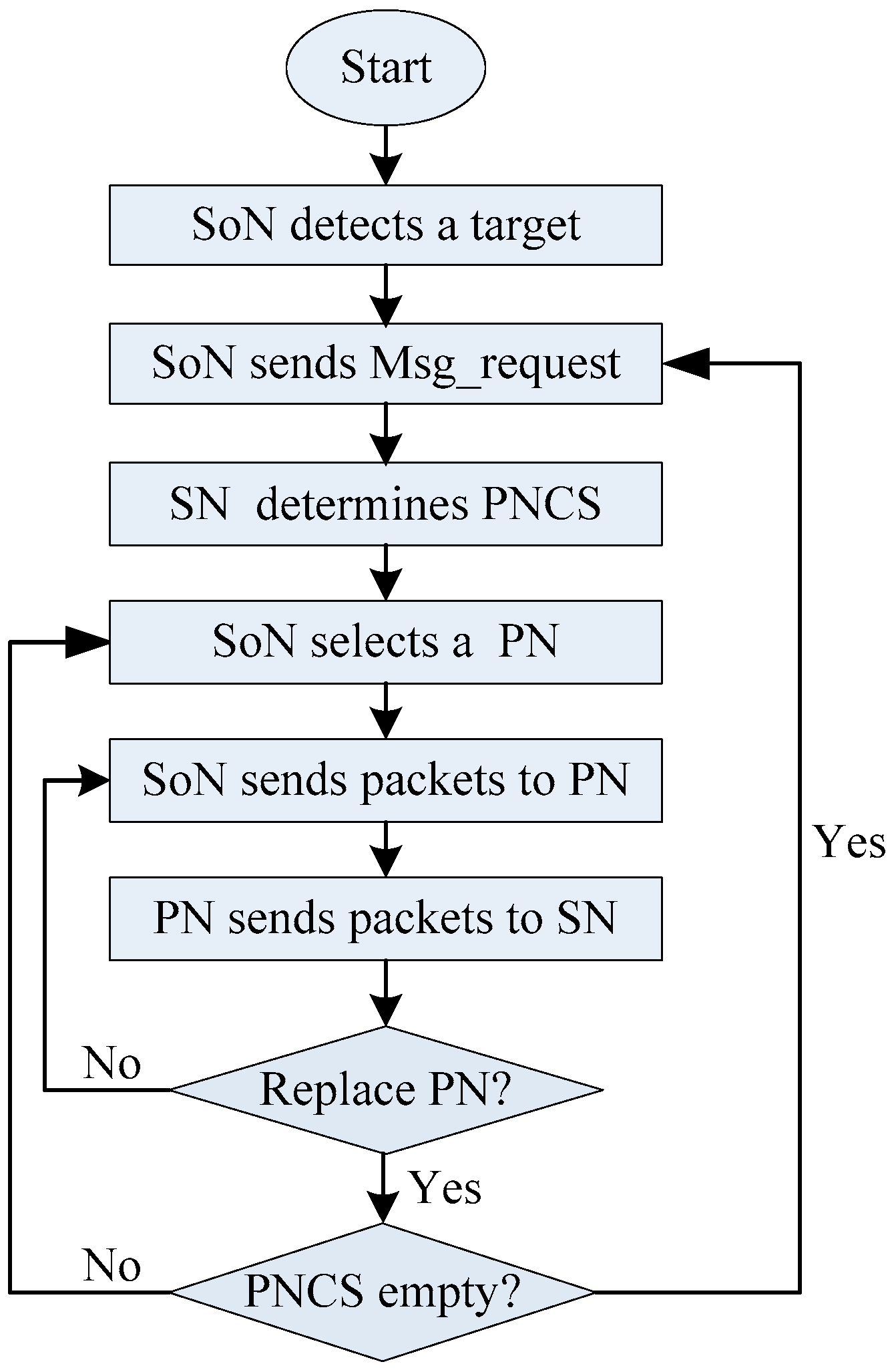
3.3. The Routing Phase
3.3.1. Step 1: The Source Node Sends Data Packets to The Phantom Node
3.3.2. Step 2: The Phantom Node Sends Data Packets to The Sink Node
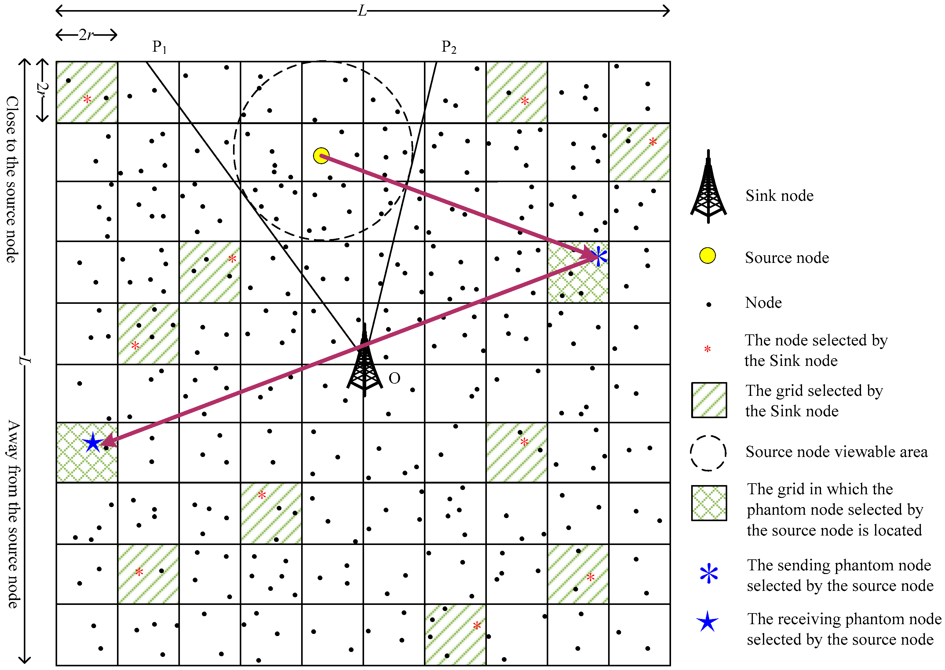
4. DPS: Grid-Based Dual Phantom Node Source Location Privacy Protection Scheme
4.1. The Initialization Phase
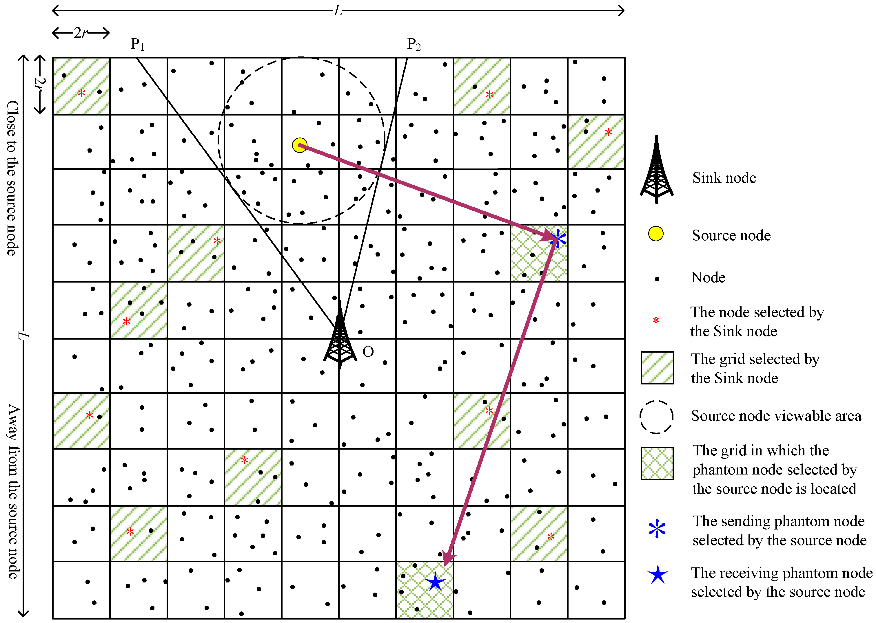
4.2. The Phantom Node Determination Phase
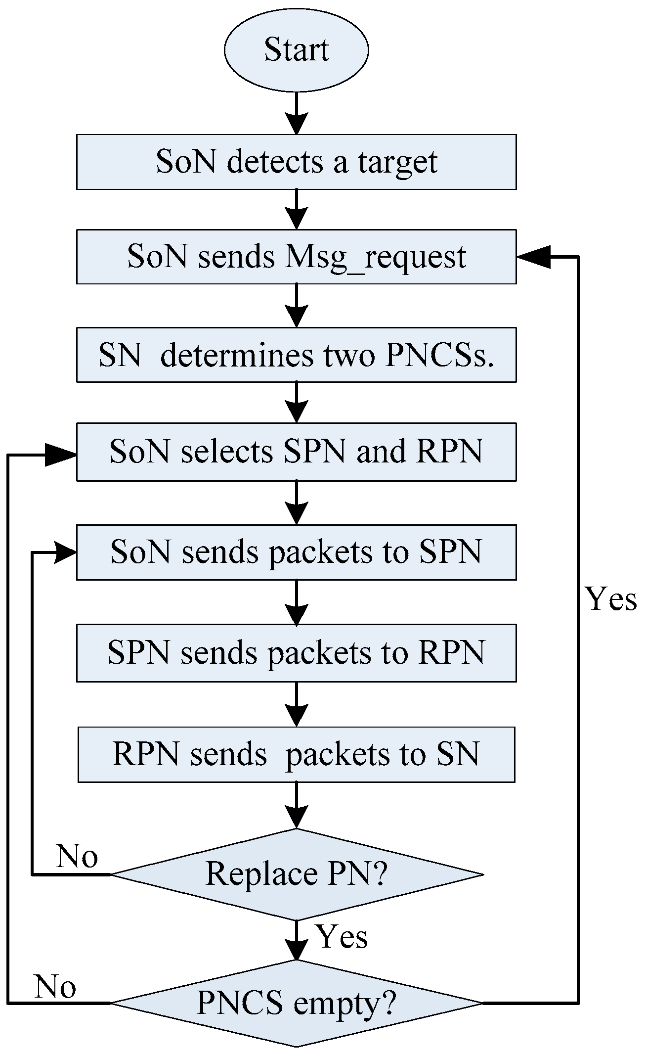
4.3. The Routing Phase
5. Performance Analysis and Simulation
5.1. Security Performance Analysis
5.1.1. Security Performance Analysis of EPUSBRF, RPBMP and Shortest Path Algorithms
5.1.2. Security Performance Analysis of our Proposed Schemes
5.1.3. Comparison of Security Performance
5.2. Analysis of Communication Overhead
5.2.1. Communication Overhead of the Phantom Node Determination Phase
5.2.2. Communication Overhead of the Routing Phase
5.2.3. Comparison of the Total Communication Overhead
5.3. Comparison of the Performance Simulation
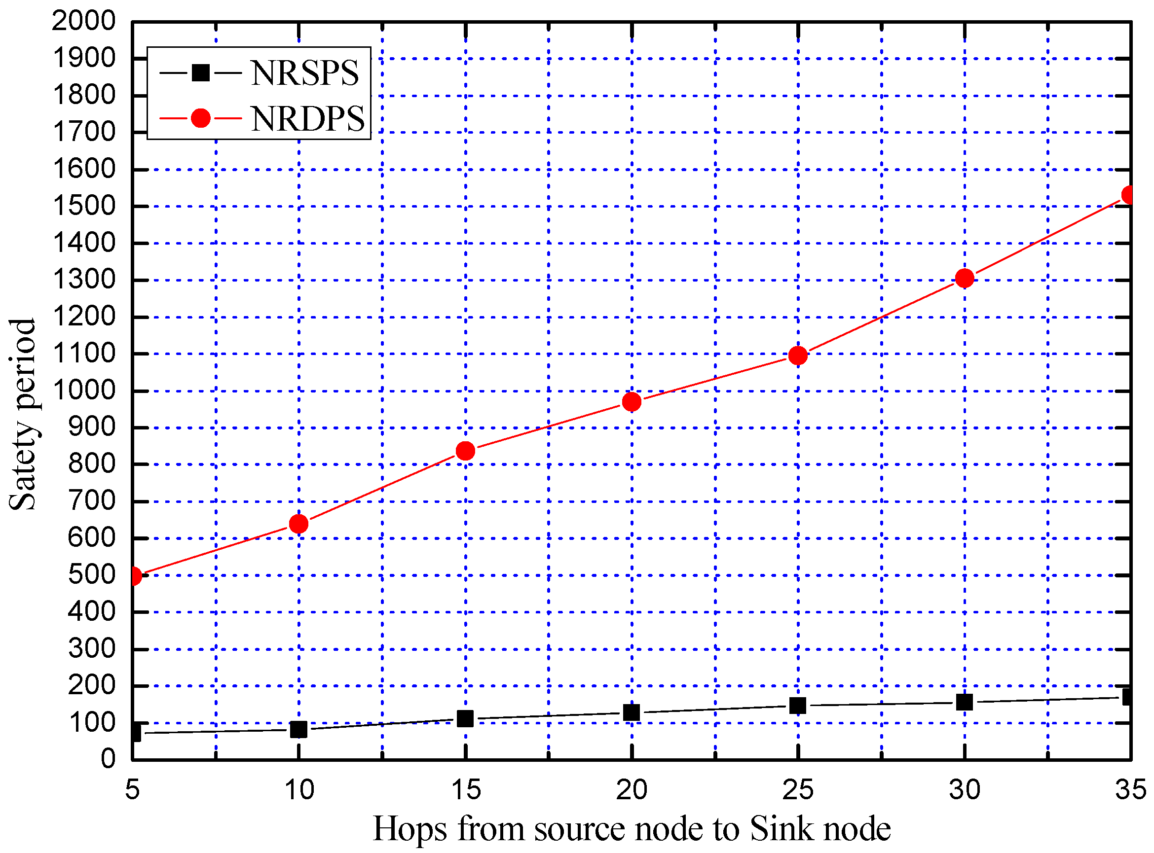
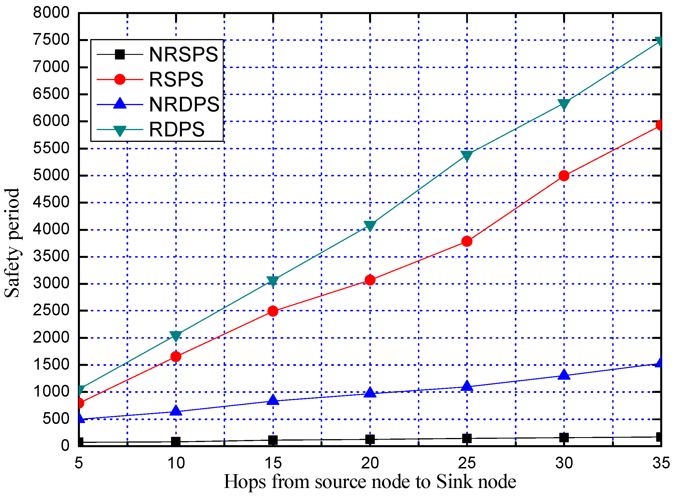
5.3.1. Comparison of Safety Period
5.3.2. Comparison of Communication Overhead
6. Conclusions
Author Contributions
Funding
Conflicts of Interest
Abbreviations
| SPS | grid-based Single Phantom node source location privacy protection Scheme |
| DPS | grid-based Dual Phantom node source location privacy protection Scheme |
| WSNs | Wireless Sensor Networks |
| SN | Sink Node |
| PN | Phantom Node |
| PNCS | Phantom Node Candidate Set |
| IoT | Internet of Things |
| SoN | Source Node |
| PRS | Phantom Routing Scheme |
| PSRS | Phantom Single-path Routing Scheme |
| EPUSBRF | Enhanced source location privacy preservation Protocol Using Source-Based Restricted Flooding |
| RPBMP | source location privacy preservation Routing Protocol Based on Multi-Path |
| PRABNS | Phantom Routing based on Area and Brother Neighbor Selecting |
| RSPS | SPS scheme in the case of Replacing the phantom node |
| RDPS | DPS scheme in the case of Replacing the phantom node |
| NRSPS | SPS scheme in the case of Not Replacing the phantom node |
| NRDPS | DPS scheme in the case of Not Replacing the phantom node |
| SPN | Sending Phantom Node |
| RPN | Receiving Phantom Node |
| SPNCS | Sending Phantom Node Candidate Set |
| RPNCS | Receiving Phantom Node Candidate Set |
| Hops,p | Hop count from the Source node to the Phantom node in the EPUSBRF scheme |
| Hopp,sink | Hop count from the Phantom node to the Sink node in the EPUSBRF scheme |
| Hop’s,p | Hop count from the Source node to the Phantom node in the RPBMP scheme |
| Hop’p,sink | Hop count from the Phantom node to the Sink node in the RPBMP scheme |
| Hops,sink | Hop count from the Source node to the Sink node in the shortest path algorithm |
| HopEPUSBRF | routing path Hop in the EPUSBRF scheme |
| HopRPBMP | routing path Hop in the RPBMP scheme |
| HopShortest | routing path Hop in the Shortest path algorithm |
| TEPUSBRF | Time required for the attacker to trace back to the source node in the EPUSBRF scheme |
| TRPBMP | Time required for the attacker to trace back to the source node in the RPBMP scheme |
| TShortest | Time required for the attacker to trace back to the source node in the Shortest path algorithm |
| Tpp | Phantom node usage Time |
| Hops,ps | Hop count from the Source node to the Phantom node in the NRSPS and NRDPS scheme |
| Hopps,sink | Hop count from the Phantom node to the Sink node in the NRSPS scheme |
| Hopps,pr | Hop count from the Sending Phantom node to the Receiving Phantom node in the NRDPS scheme |
| Hoppr,sink | Hop count from the Receiving Phantom node to the Sink node in the NRDPS scheme |
| TNRSPSp | Time required for the attacker to trace to the Phantom node in the NRSPS scheme |
| TNRSPSs | Time required for the attacker to trace to the Source node in the NRSPS scheme |
| TNRDPSp | Time required for the attacker to trace to the Phantom node in the NRDPS scheme |
| TNRDPSs | Time required for the attacker to trace to the Source node in the NRDPS scheme |
| TNRSPSpp | Phantom node usage Time in the NRSPS scheme |
| TNRDPSpp | Phantom node usage Time in the NRDPS scheme |
| HopNRSPSsum | Hops of routing path in the NRSPS scheme |
| HopNRDPSsum | Hops of routing path in the NRDPS scheme |
| Hoppc,sink | Hop count from the Phantom node to the Sink node in the NRSPS, NRDPS, EPUSBRF and RPBMP scheme |
| TEPUSBRFt | Time required for the attacker to trace to the phantom node in the EPUSBRF scheme |
| TRPBMPt | Time required for the attacker to trace to the phantom node in the RPBMP scheme |
| TNRSPSt | Time required for the attacker to trace to the phantom node in the NRSPS scheme |
| TNRDPSt | Time required for the attacker to trace to the phantom node in the NRDPS scheme |
| TRSPSt | Time required for the attacker to trace to the last phantom node in the RSPS scheme |
| TRDPSt | Time required for the attacker to trace to the last phantom node in the RDPS scheme |
| HoppEPUSBRF | communication overhead of determining Phantom node in the EPUSBRF scheme |
| HoppRPBMP | communication overhead of determining Phantom node in the RPBMP scheme |
| HoppShortest | communication overhead of determining Phantom node in the Shortest path algorithm |
| HoppSPS | communication overhead of determining Phantom node in the SPS scheme |
| HoppDPS | communication overhead of determining Phantom node in the DPS scheme |
| HopEPUSBRFc | Communication overhead of the EPUSBRF scheme in the routing phase |
| HopRPBMPc | Communication overhead of the RPBMP scheme in the routing phase |
| HopNRSPSc | Communication overhead of the NRSPS scheme in the routing phase |
| HopRSPSc | Communication overhead of the RSPS scheme in the routing phase |
| HopNRDPSc | Communication overhead of the NRDPS scheme in the routing phase |
| HopRDPSc | Communication overhead of the RDPS scheme in the routing phase |
| HopEPUSBRFsum | Sum of the communication overheads in the EPUSBRF scheme |
| HopRPBMPsum | Sum of the communication overheads in the RPBMP scheme |
| HopRDPSsum | Sum of the communication overheads in the RDPS scheme |
| HopNRDPSsum | Sum of the communication overheads in the NRDPS scheme |
| HopRSPSsum | Sum of the communication overheads in the RSPS scheme |
| HopNRSPSsum | Sum of the communication overheads in the NRSPS scheme |
References
- Wang, J.; Wang, F.; Cao, Z.; Lin, F.; Wu, J. Sink Location Privacy Protection under Direction Attack in Wireless Sensor Networks. Wirel. Netw. 2016, 23, 579–591. [Google Scholar] [CrossRef]
- Jia, Z.; Wei, X.; Guo, H.; Peng, W.; Song, C. A Privacy Protection Strategy for Source Location in WSN Based on Angle and Dynamical Adjustment of Node Emission Radius. Chin. J. Electron. 2017, 26, 1064–1072. [Google Scholar] [CrossRef]
- Mutalemwa, L.C.; Shin, S. A New Diversional Routing Scheme to Preserve Source Location Privacy in Wireless Sensor Networks. In Proceedings of the 3rd International Conference on Next Generation Computing (ICNGC2017b), Kaohsiung, Taiwan, 21–23 December 2017; pp. 260–262. [Google Scholar]
- Li, Y.; Lightfoot, L.; Ren, J. Routing-based Source-Location Privacy Protection in Wireless Sensor Networks. In Proceedings of the IEEE International Conference on Electro/Information Technology, Windsor, ON, Canada, 7–9 June 2009; pp. 29–34. [Google Scholar]
- Kirton, J.; Bradbury, M.S.; Jhumka, A. Source Location Privacy-Aware Data Aggregation Scheduling for Wireless Sensor Networks. In Proceedings of the 37th IEEE International Conference on Distributed Computing Systems, Atlanta, GA, USA, 5–8 June 2017; pp. 2200–2205. [Google Scholar]
- Ozturk, C.; Zhang, Y.; Trappe, W.; Ott, M. Source-Location Privacy for Networks of Energy-Constrained Sensors. In Proceedings of the Second IEEE Workshop on Software Technologies for Future Embedded and Ubiquitous Systems, Vienna, Austria, 12 May 2004; pp. 68–72. [Google Scholar]
- Kamat, P.; Zhang, Y.; Trappe, W.; Ozturk, C. Enhancing Source-Location Privacy in Sensor Network Routing. In Proceedings of the IEEE international conference on distributed computing systems (ICDCS’05), Columbus, OH, USA, 6–10 June 2005; pp. 599–608. [Google Scholar]
- Lilian, C.M.; Seokjoo, S. Strategic Location-Based Random Routing for Source Location Privacy in Wireless Sensor Networks. Sensors 2018, 18, 2291. [Google Scholar]
- WWWF—The conservation organization. Available online: http://www.panda.org/ (accessed on 3 March 2019).
- Wang, H.D.; Sheng, B.; Li, Q. Privacy-Aware Routing in Sensor Networks. Comput. Networks 2009, 53, 1512–1529. [Google Scholar] [CrossRef]
- Ouyang, Y.; Le, Z.; Chen, G.; James, F.; Fillia, M. Entrapping Adversaries for Source Protection in Sensor Networks. In Proceedings of the International Symposium on World of Wireless, Mobile and Multimedia Networks, Washington, DC, USA, 26–29 June 2006; pp. 23–34. [Google Scholar]
- Tan, W.; Xu, K.; Wang, D. An anti-tracking source-location privacy protection protocol in WSNs based on path extension. IEEE Internet Things J. 2014, 1, 461–471. [Google Scholar] [CrossRef]
- Yi, X.F.; Fan, X.P. Redundancy Branch Combine Spiral Routing to Preserve Source Location Privacy for WSNs. J. Chin. Comput. Syst. 2015, 36, 244–251. (In Chinese) [Google Scholar]
- Roy, P.; Rimjhim; Singh, J.P.; Kumar, P. An efficient privacy preserving protocol for source location privacy in wireless sensor networks. In Proceedings of the International Conference on Wireless Communications, Signal Processing and Networking (WiSPNET), Chennai, India, 23–25 March 2016; pp. 1093–1097. [Google Scholar]
- Zhang, J.N.; Chu, C.L. A Scheme to Protect the Source Location Privacy in Wireless Sensor Networks. Chin. J. Sens. Actuators 2016, 29, 1405–1409. (In Chinese) [Google Scholar]
- Ma, W.; Song, L. Source location privacy preservation routing protocol based on multi-path. Comput. Eng. Appl. 2018, 54, 81–85. (In Chinese) [Google Scholar]
- Ozturk, C.; Zhang, Y.; Trappe, W. Source-location privacy in energy-constrained sensor network routing. In Proceedings of the 2nd ACM workshop on Security of ad hoc and sensor networks, Washington, DC, USA, 25–25 October 2004; pp. 88–93. [Google Scholar]
- Chen, J.; Fang, B.X.; Yin, L.H.; Su, S. A Source-Location Privacy Preservation Protocol in Wireless Sensor Networks Using Source-Based Restricted Flooding. Chin. J. Comput. 2010, 33, 1736–1747. (In Chinese) [Google Scholar] [CrossRef]
- Yi, X.F.; Fan, X.P. Beyond Adversary Trace Time Routing Approach for Preserving Source-location in WSNs. J. Chin. Comput. Syst. 2014, 35, 311–318. (In Chinese) [Google Scholar]
- Chen, Y.; Jiang, C.H.; Guo, C.; Xie, F.Y.; Wu, H.C. An Improved Routing Algorithm for Source Location Privacy Protection in Wireless Sensor Network. Chin. J. Sens. Actuators 2017, 30, 438–449. (In Chinese) [Google Scholar]
- Kong, X.X.; Yuan, S.Q.; Chen, M. Routing Protocol of Source-Location Privacy Protection based on Virtual Ring. Transducer Microsyst. Technol. 2018, 37, 66–69. (In Chinese) [Google Scholar]
- Wang, W.X.; Li, P.Z. A Privacy Protection Method of Source Location in Wireless Sensor Networks. J. Chongqing Univ. 2018, 41, 100–108. (In Chinese) [Google Scholar]
- Cerpa, A.; Estrin, D. ASCENT: Adaptive Self-Configuring Sensor Networks Topologies. IEEE Trans. Mob. Comput. 2004, 3, 272–285. [Google Scholar] [CrossRef]
- Chai, R.; Zhang, Y. A Practical Supercapacitor Model for Power Management in Wireless Sensor Nodes. IEEE Trans. Power Electron. 2015, 30, 6720–6730. [Google Scholar] [CrossRef]
- Jiang, J.; Han, G.; Wang, H.; Guizani, M. A survey on location privacy protection in Wireless Sensor Networks. J. Networks Comput. Appl. 2019, 125, 93–114. [Google Scholar] [CrossRef]
- Bradbury, M.; Jhumka, A.; Leeke, M. Hybrid Online Protocols for Source Location Privacy in Wireless Sensor Networks. J. Parallel Distrib. Comput. 2018, 115, 67–81. [Google Scholar] [CrossRef]
- Intanagonwiwat, C.; Govindan, R.; Estrin, D. Directed Diffusion: A Scalable and Robust Communication Paradigm for Sensor Networks. In Proceedings of the Sixth Annual ACM/IEEE International Conference on Mobile Computing and Networks (MobiCOM), Boston, MA, USA, 6–11 August 2000; pp. 56–67. [Google Scholar]
- Olasupo, T.O.; Otero, C.E. The Impacts of Node Orientation on Radio Propagation Models for Airborne-Deployed Sensor Networks in Large-Scale Tree Vegetation Terrains. IEEE Trans. Syst. Man Cybern. Part A Syst. 2017, 1–14. [Google Scholar] [CrossRef]


| Notations | Description |
|---|---|
| U | Node u |
| Hopu,sink | Minimum hop count between node u and sink node |
| L*L | Network size |
| R | Node communication radius |
| i, j, m, n | Grid number index variable |
| Grid number of the i-th row and the j-th column |
| Node ID | Minimum Hop Count from Sink Node | Grid Number |
|---|---|---|
| u | ||
| … | … | … |
| Scheme | Total Communication Overhead |
|---|---|
| EPUSBRF | |
| RPBMP | |
| Shortest path algorithm | |
| NRSPS | |
| NRDPS | |
| RSPS | |
| RDPS |
| Overhead 1 | Overhead 2 | Total Overhead | Total Safety Period | SC Ratio | ||
|---|---|---|---|---|---|---|
| Shortest path | 0 | 20.93 | 20.93 | 20.93 | 1 | |
| RPBMP | 30 | 335.76 | 365.76 | 45.68 | 0.12 | |
| EPUSBRF | 731.26 | 87.05 | 818.31 | 35.68 | 0.04 | |
| Proposed | NRSPS | 0 | 43.18 | 43.18 | 127.21 | 0.34 |
| RSPS | 0 | 959.62 | 959.62 | 3070 | 3.20 | |
| NRDPS | 0 | 323.04 | 323.04 | 969 | 3.00 | |
| RDPS | 0 | 2292.60 | 2292.60 | 4087 | 1.78 | |
© 2019 by the authors. Licensee MDPI, Basel, Switzerland. This article is an open access article distributed under the terms and conditions of the Creative Commons Attribution (CC BY) license (http://creativecommons.org/licenses/by/4.0/).
Share and Cite
Wang, Q.; Zhan, J.; Ouyang, X.; Ren, Y. SPS and DPS: Two New Grid-Based Source Location Privacy Protection Schemes in Wireless Sensor Networks. Sensors 2019, 19, 2074. https://doi.org/10.3390/s19092074
Wang Q, Zhan J, Ouyang X, Ren Y. SPS and DPS: Two New Grid-Based Source Location Privacy Protection Schemes in Wireless Sensor Networks. Sensors. 2019; 19(9):2074. https://doi.org/10.3390/s19092074
Chicago/Turabian StyleWang, Qiuhua, Jiacheng Zhan, Xiaoqin Ouyang, and Yizhi Ren. 2019. "SPS and DPS: Two New Grid-Based Source Location Privacy Protection Schemes in Wireless Sensor Networks" Sensors 19, no. 9: 2074. https://doi.org/10.3390/s19092074
APA StyleWang, Q., Zhan, J., Ouyang, X., & Ren, Y. (2019). SPS and DPS: Two New Grid-Based Source Location Privacy Protection Schemes in Wireless Sensor Networks. Sensors, 19(9), 2074. https://doi.org/10.3390/s19092074