Edge-Computing Video Analytics for Real-Time Traffic Monitoring in a Smart City


Abstract
1. Introduction
2. The Liverpool Smart Pedestrians Project
2.1. Methodology and Objectives
- Multi-modal detection and tracking: The sensors need to be able to detect and track pedestrians, vehicles and cyclists.
- Privacy compliant: As sensors are going to be deployed over a city, the sensors should be privacy compliant, meaning that no personal data should be stored or exchanged.
- Leveraging existing infrastructures: As cities already make huge investments on CCTV systems [8], the solution should take advantage of the already existing infrastructures in terms of networks and cameras. Retrofitting the existing CCTV network to collect more data has been identified as a major innovation.
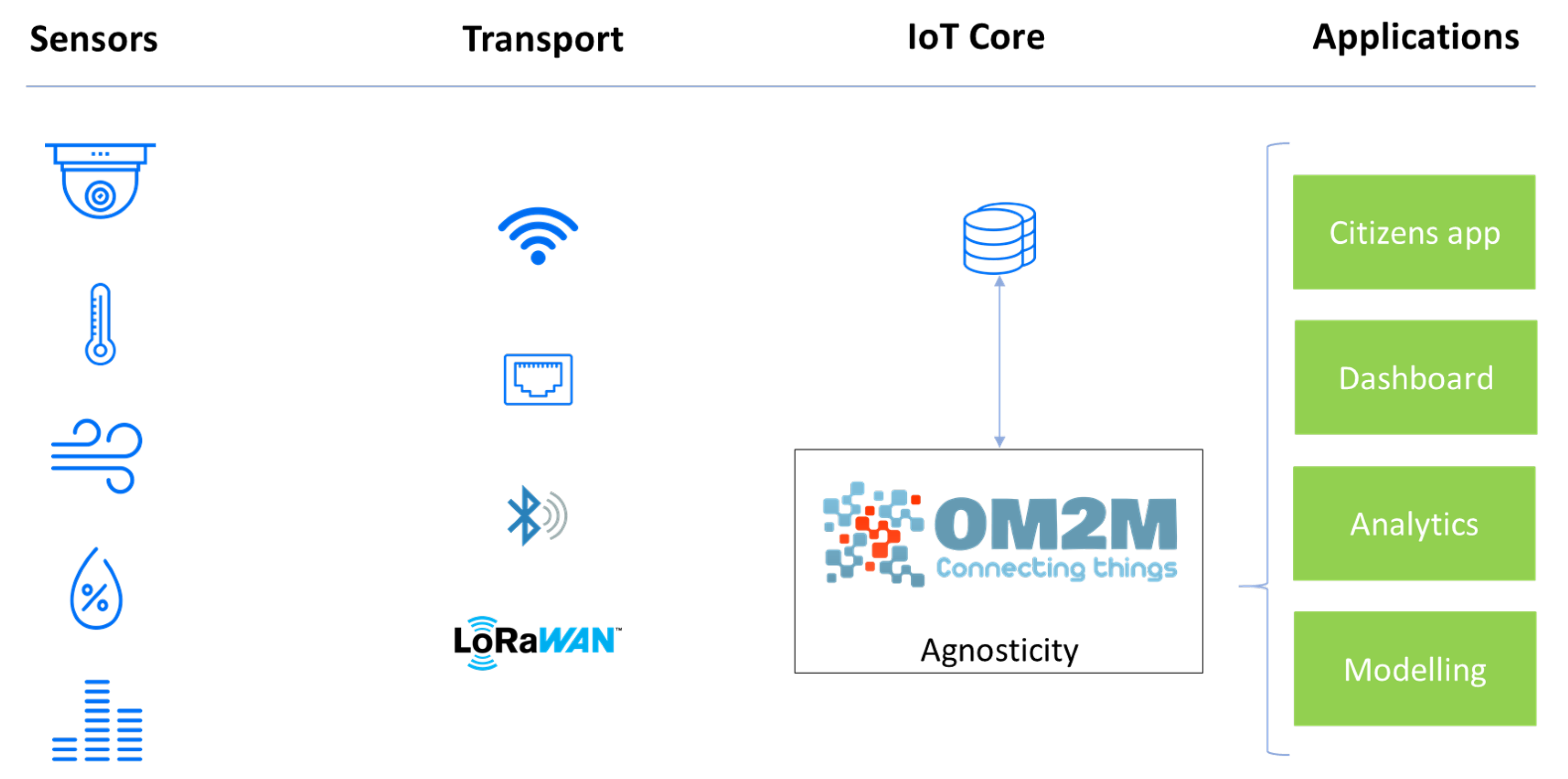
- Scalability and interoperability: New sensors can be added at any time, regardless their technologies, meaning the sensor of network can be easily expanded and capture new type of data.
2.2. Related Work
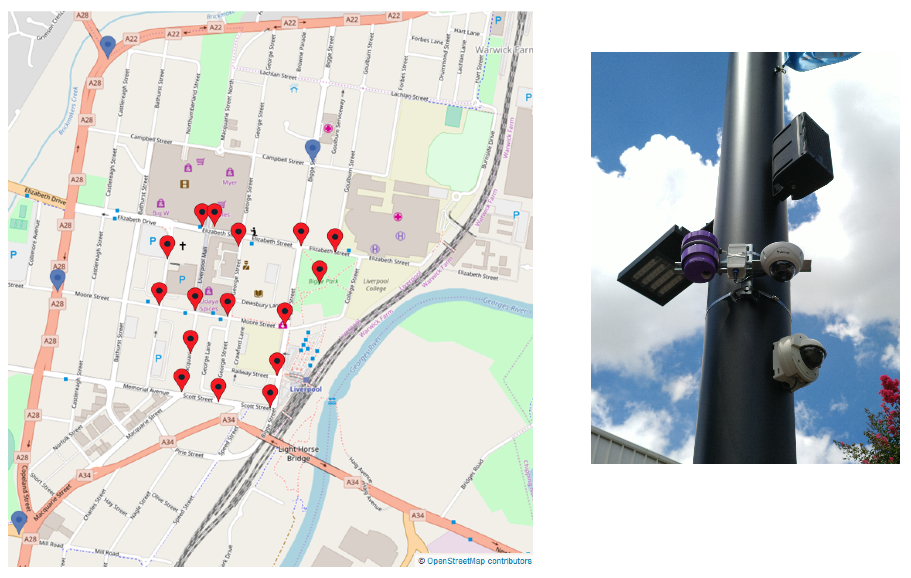
2.3. Pilot Project
3. An Edge-Computing Device for Traffic Monitoring
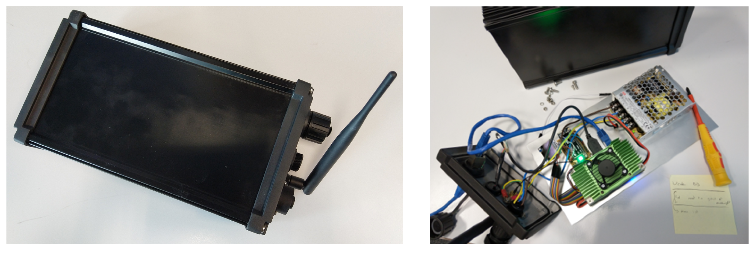
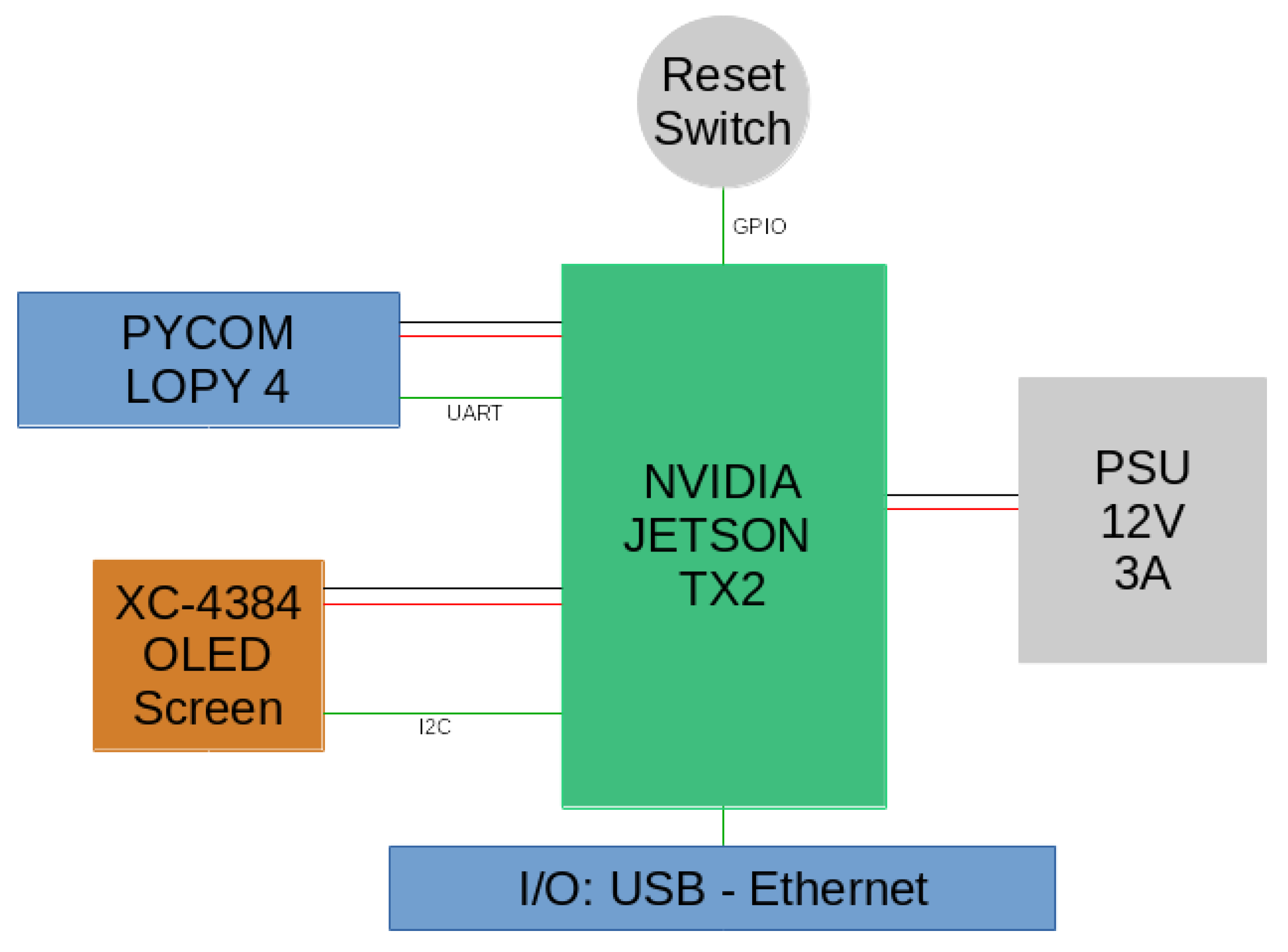
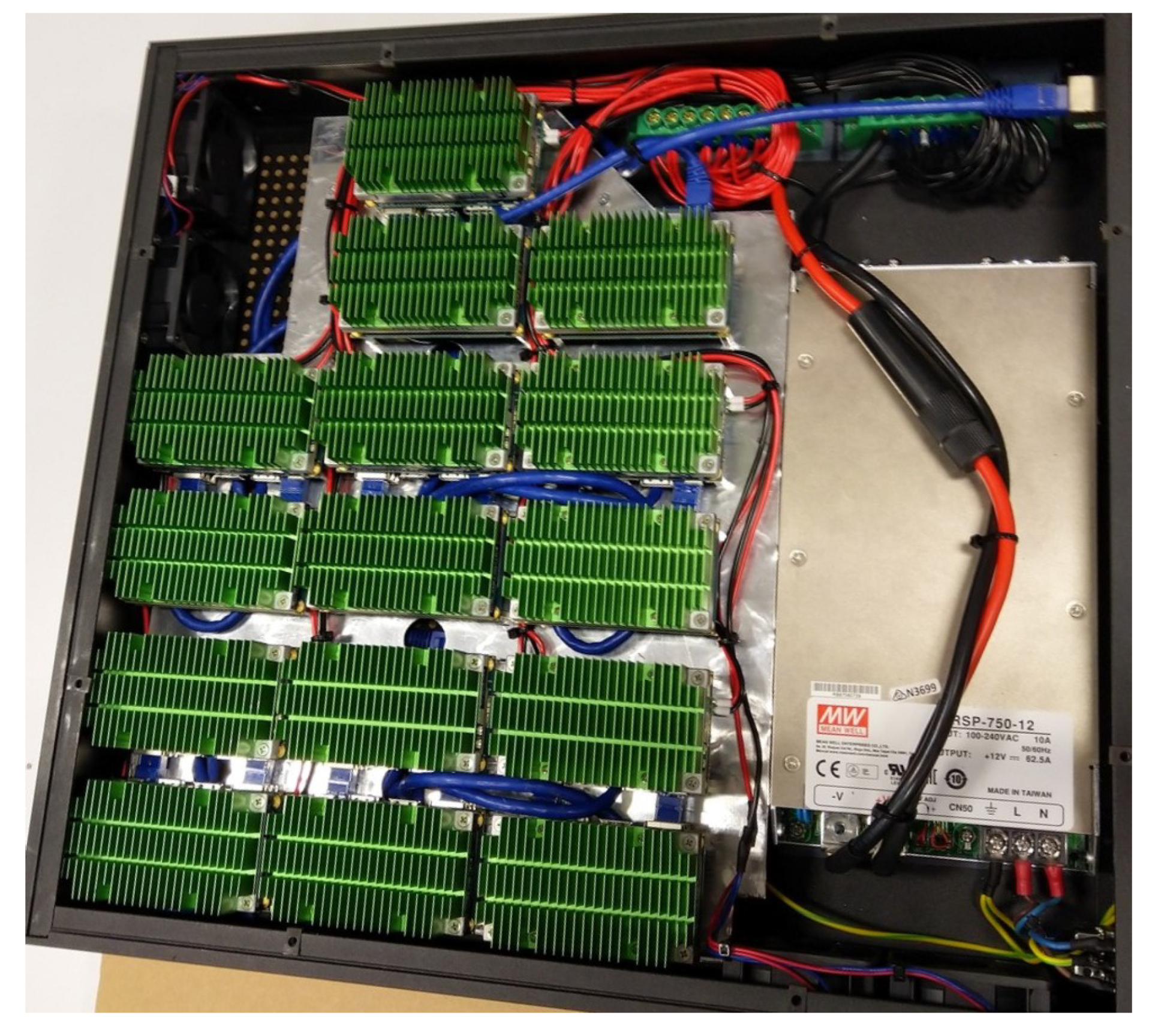
3.1. Functionality and Hardware
- it lowers the network bandwidth requirement as no raw images is transmitted, but only indicators and meta-data; and
- thanks to the limited amount of information being transmitted, the device is privacy compliant.
- an NVIDIA Jetson TX2, a high performance and power efficient ARM-based embedded computing device with specialized units for accelerating neural network computations used for image processing and running Ubuntu 16.04 LTS; and
- a Pycom LoPy 4 module handling the LoRaWAN communications on the AS923 frequency plan used in Australia. It should be noted that the module is able to transmit on every frequency plan supported by the LoRaWAN protocol.
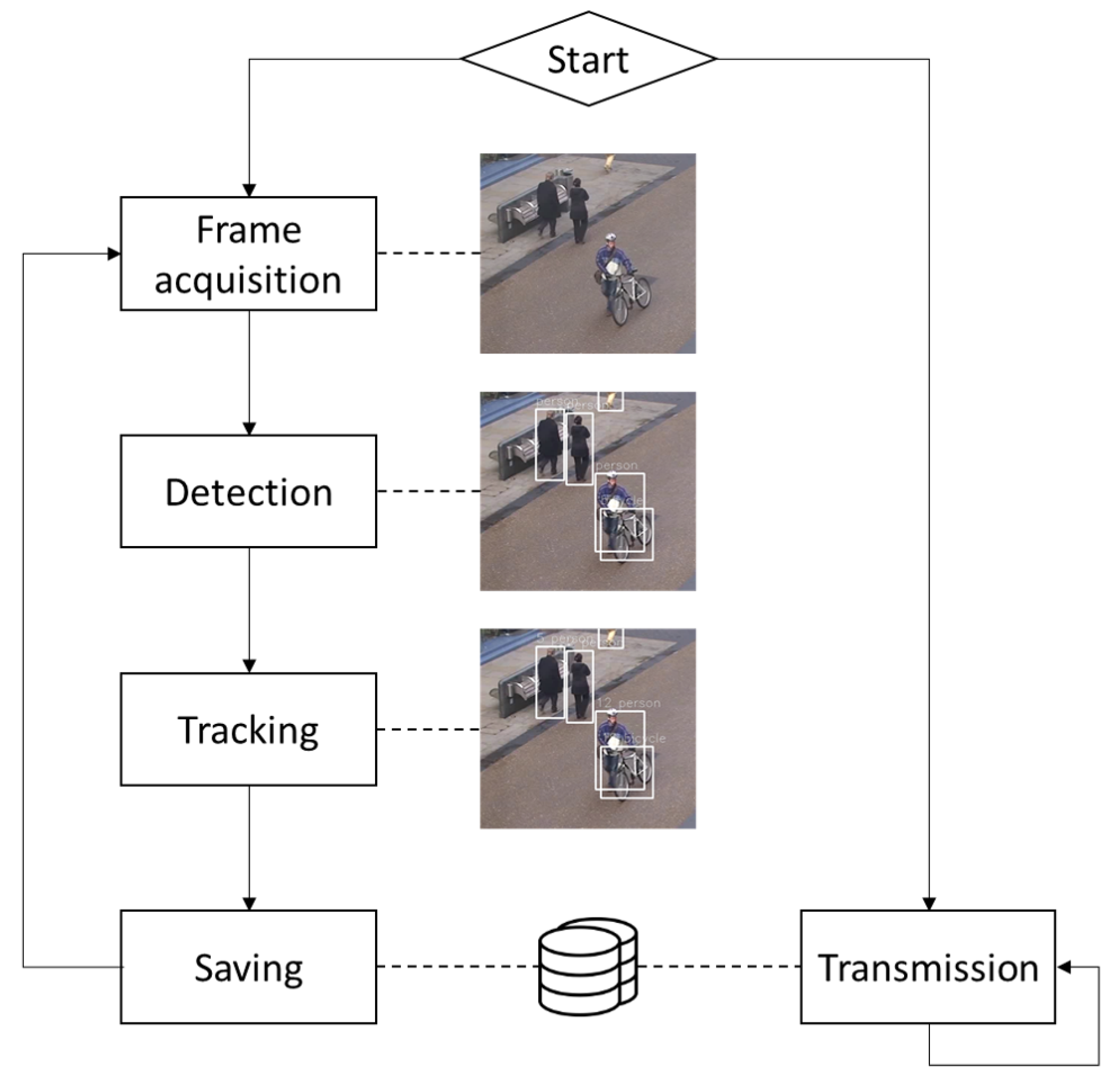
- Frame acquisition from an IP camera or an USB webcam.
- Detecting the objects of interests in the frame.
- Tracking the objects by matching the detections with the ones in the previous frame.
- Updating the trajectories of objects already stored in the device database or creating records for the newly detected objects.
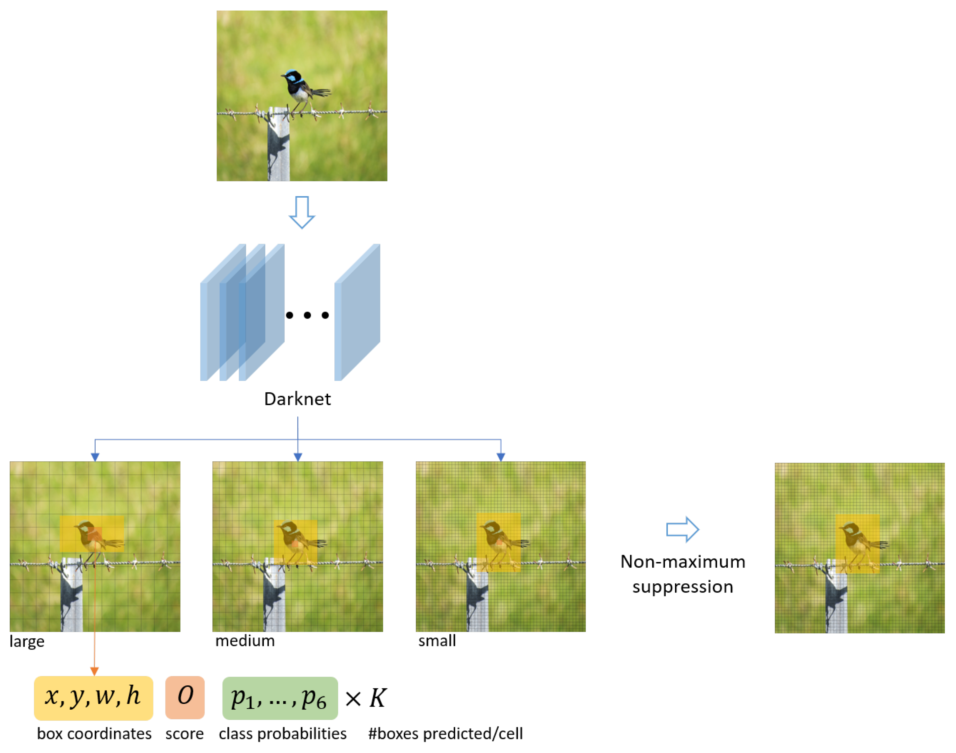
3.2. Detecting Objects: YOLO V3
| • | pedestrian | • | bus |
| • | bicycle | • | truck |
| • | car | • | motorbike |
- its shape defined by the its centroid coordinates , its width w and height h;
- an object confidence score O; and
- six class probabilities (one for each object type).
3.3. Tracking Objects: SORT
- x and y are the centroid coordinates of the object’s bounding box;
- a and s are the area and the aspect ratio of the object’s bounding box; and
- is the velocity of the feature .
4. The Agnosticity Infrastructure
5. Validation Experiments
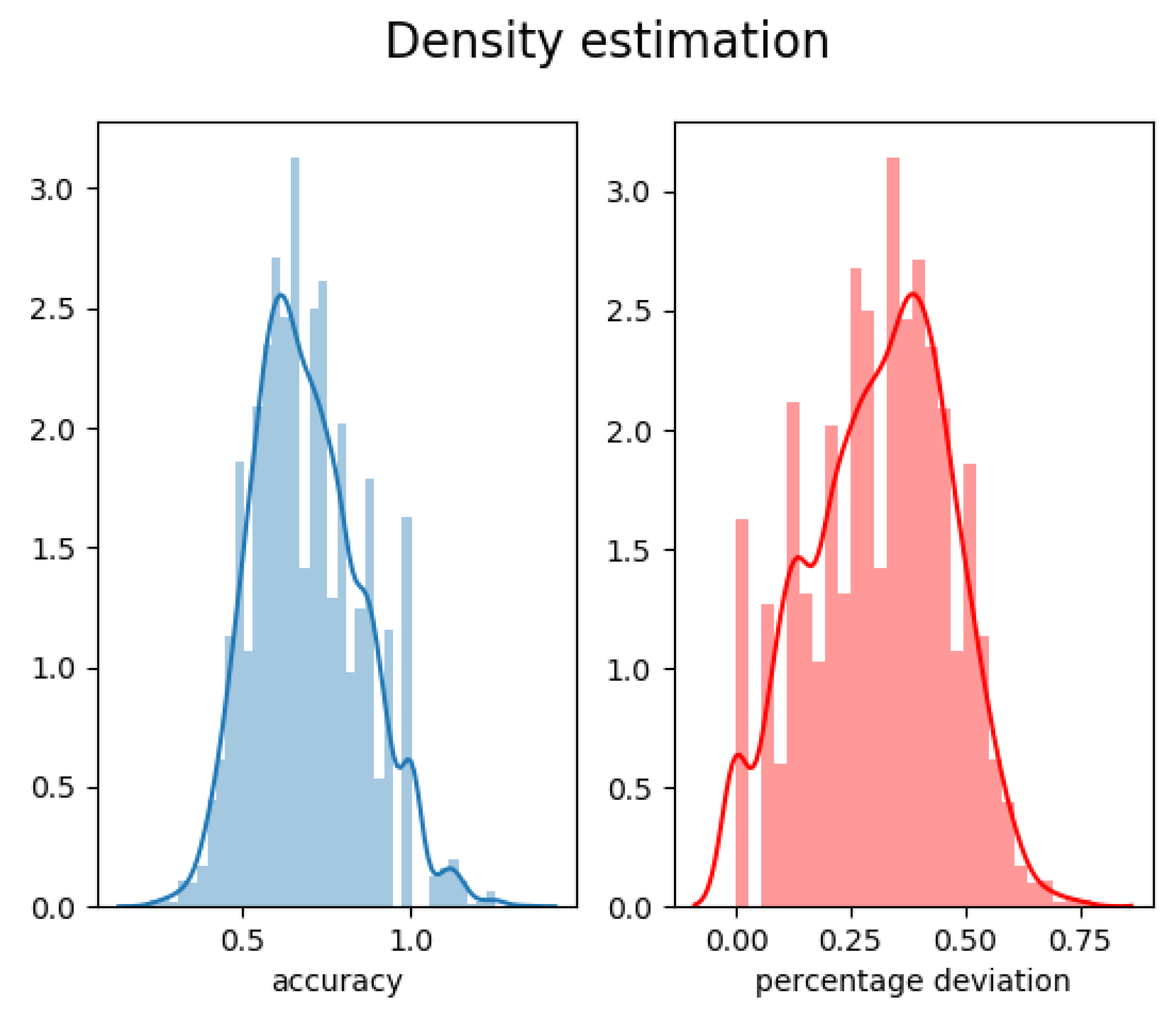
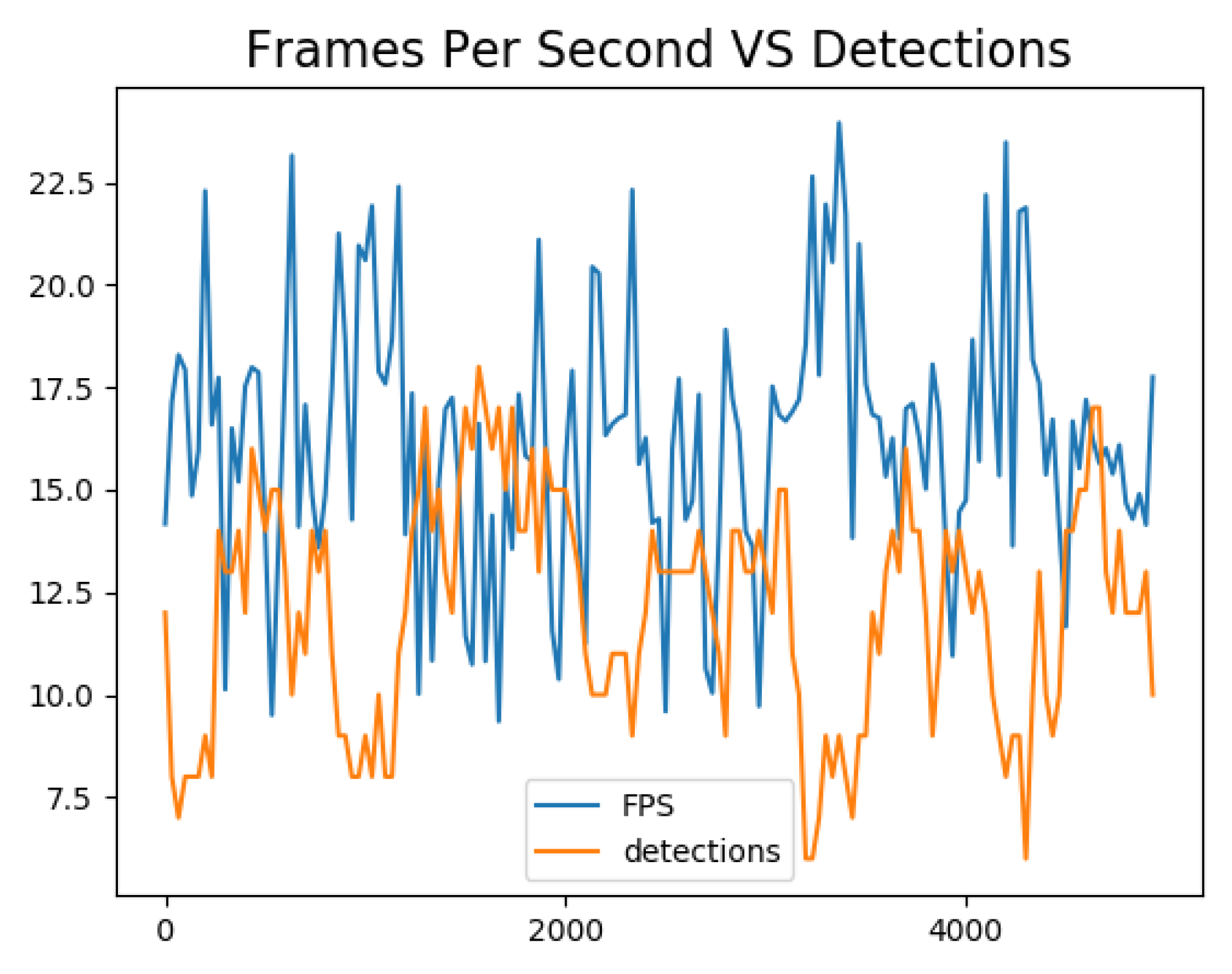
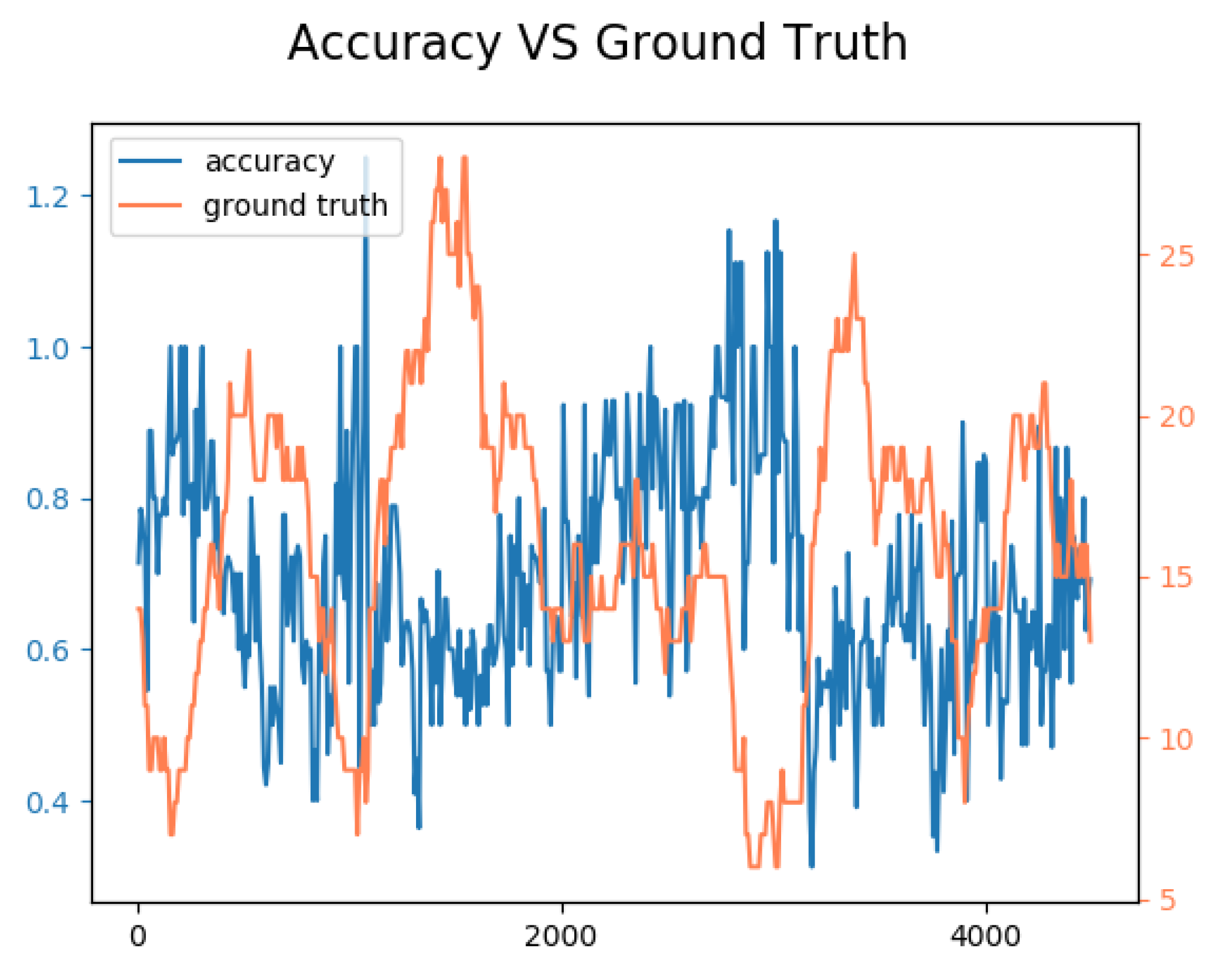
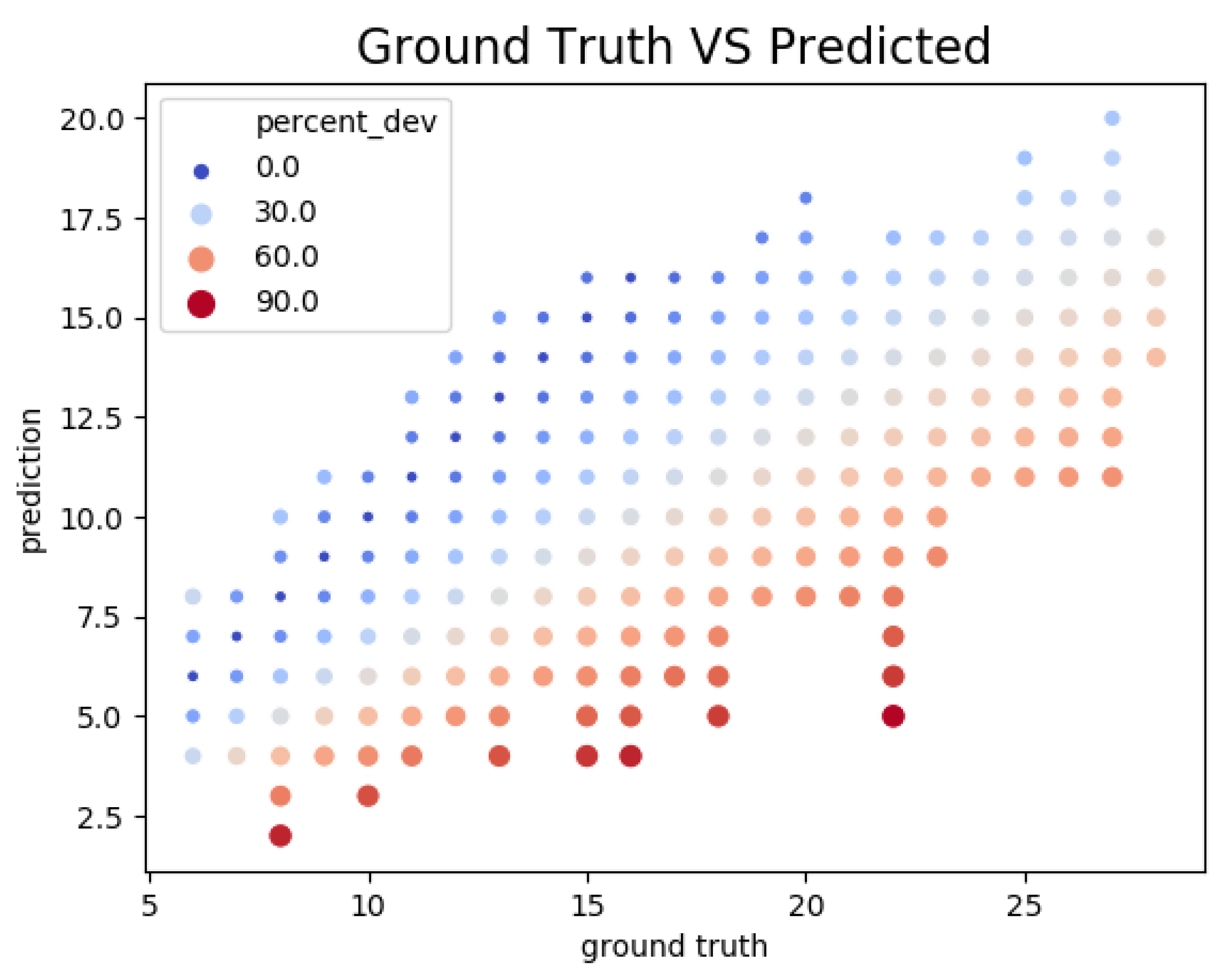
5.1. Accuracy and Performance
- : the number of objects detected by the sensor;
- : the number of object annotated in the dataset, i.e., the ground truth;
- : the difference between and ;
- : the relative error computed as:
- : the accuracy defined by:and
- : the inverse of the time required to process a frame of the video, i.e., the number of frames per second (FPS) processed by the sensor.
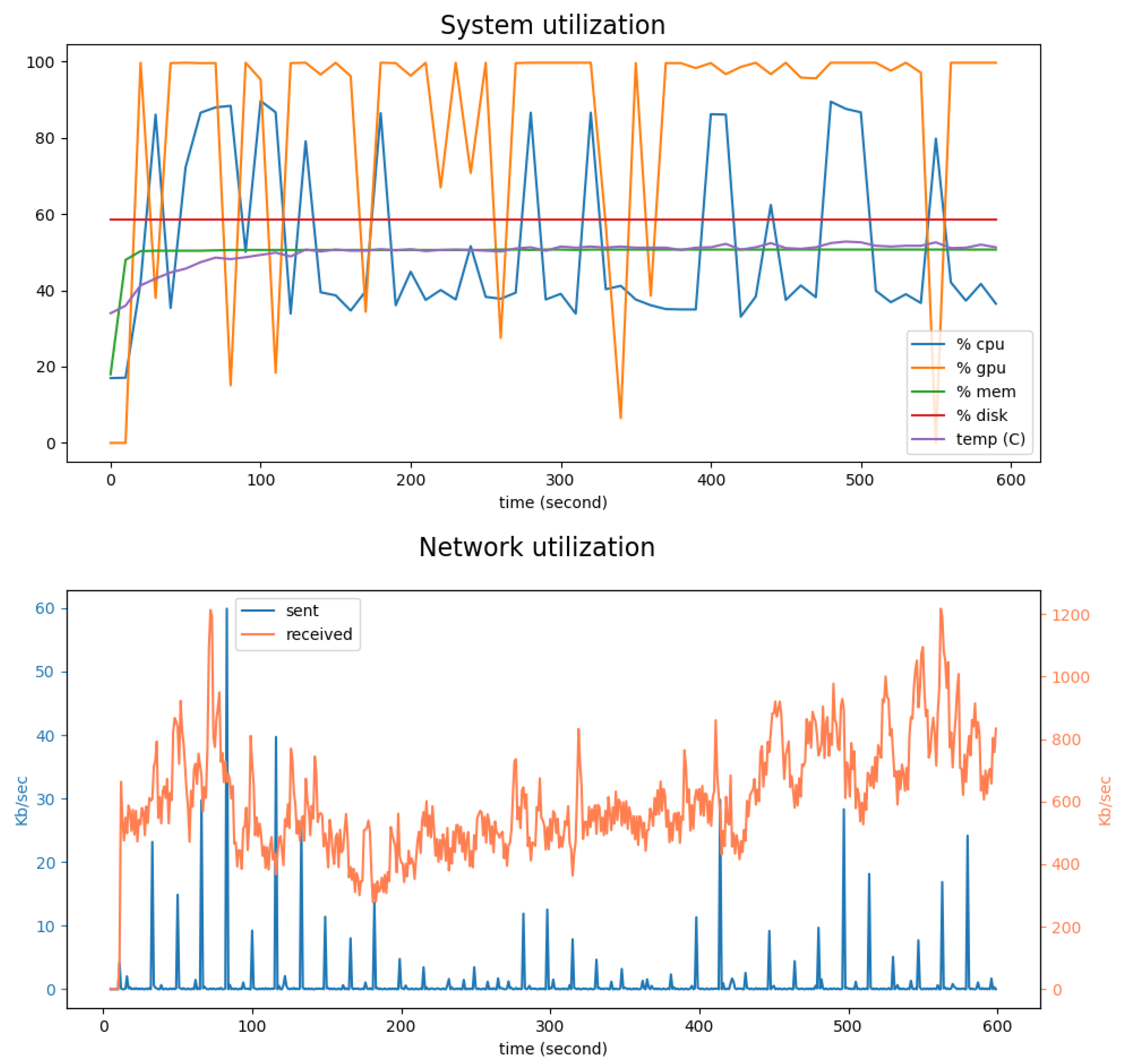
5.2. System and Network Utilization
6. Applications
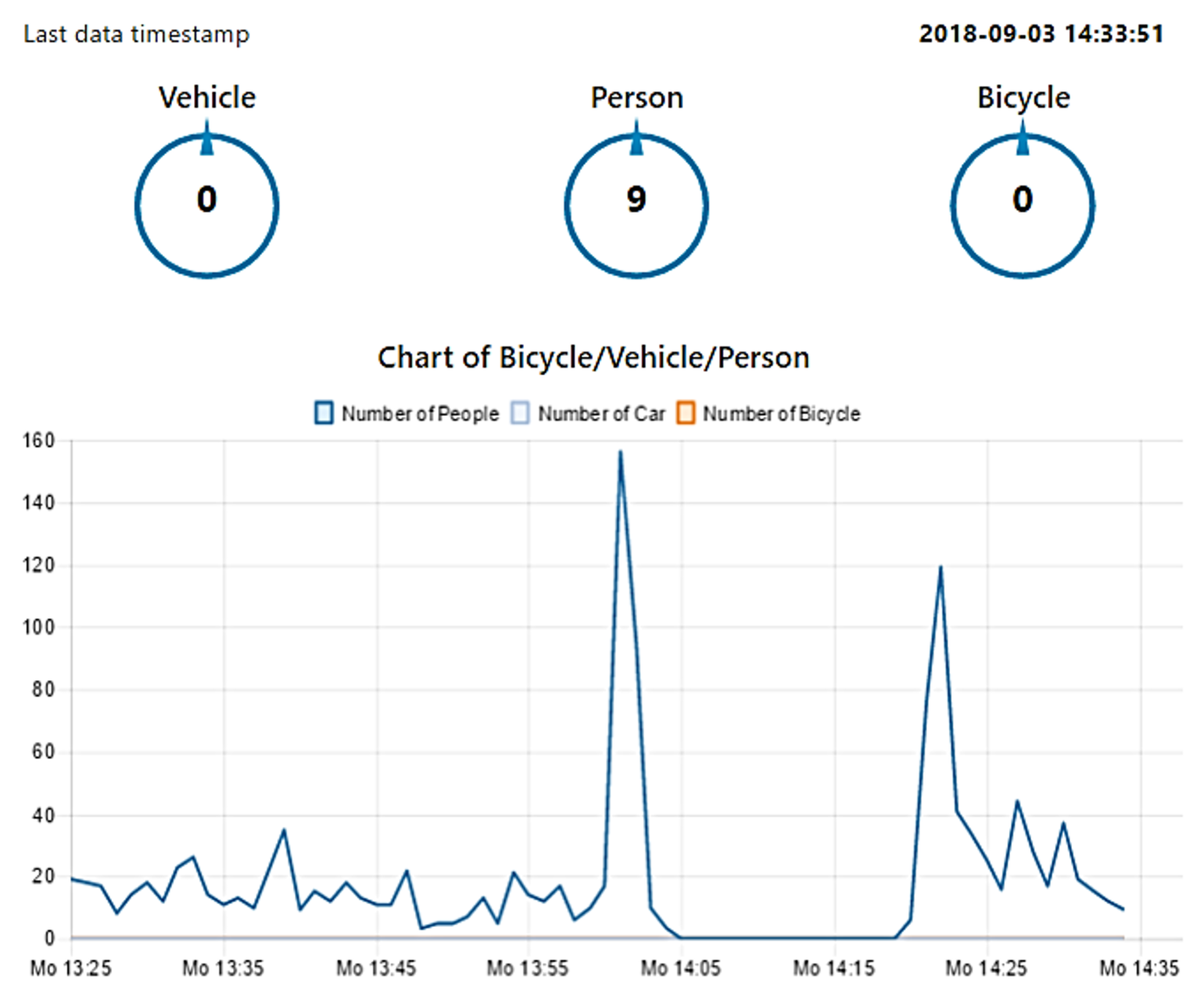
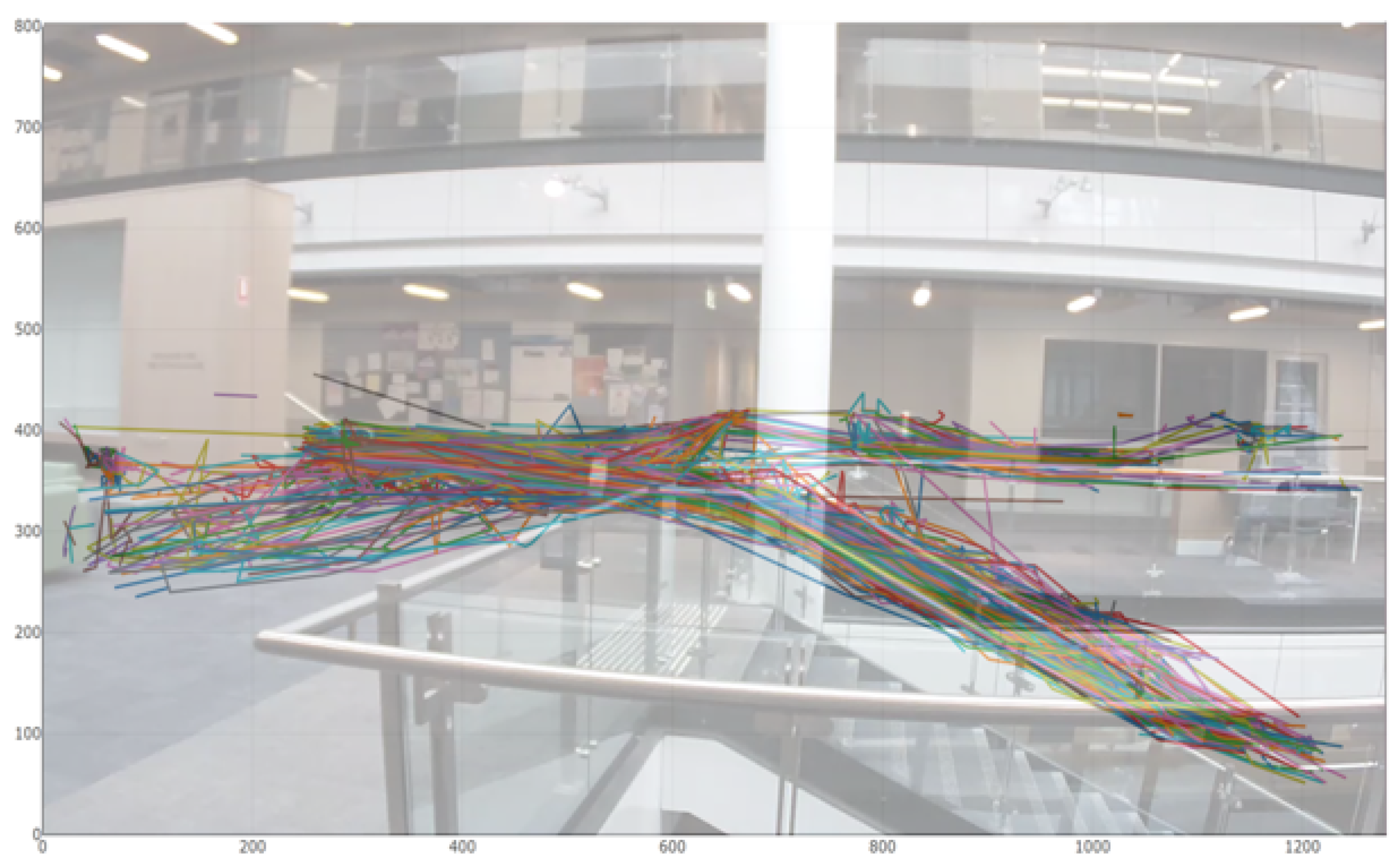
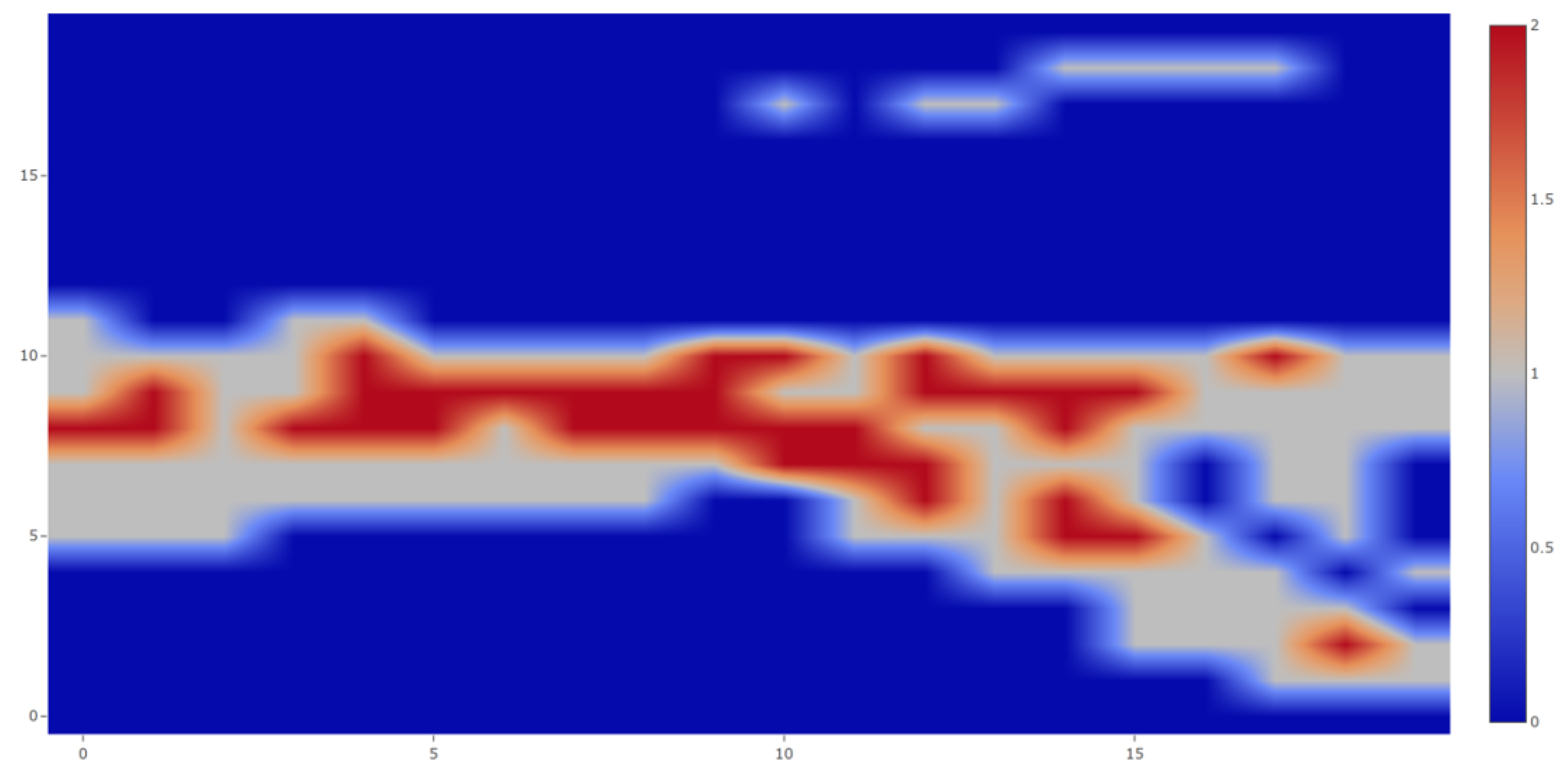
6.1. Indoor Deployment
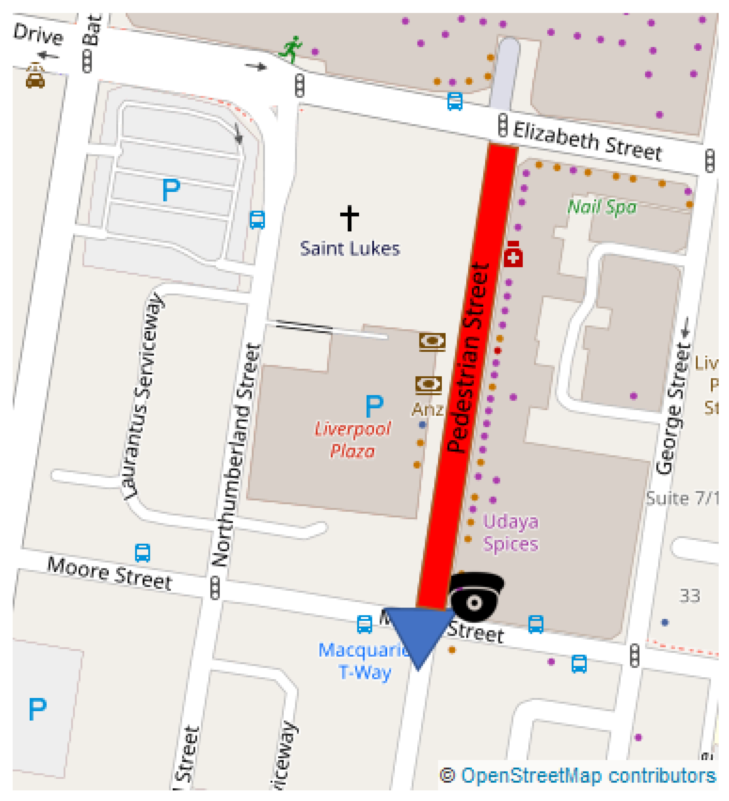
6.2. Outdoor Deployment: Liverpool
7. Conclusions and Future Work
Author Contributions
Funding
Acknowledgments
Conflicts of Interest
Appendix A. Technical Specifications

| Feature | Detail |
|---|---|
| CPU | ARM Cortex-A57 (quad-core) @ 2 GHz + NVIDIA Denver2 (dual-core) @ 2 GHz |
| GPU | 256-core Pascal @ 1300 MHz |
| Memory | 8 GB 128-bit LPDDR4 @ 1866 Mhz | 59.7 GB/s |
| Storage | 32 GB eMMC 5.1, SDIO, SATA |
| Decoder | 4 K × 2 K 60 Hz Decode (12-Bit Support) |
| Supported video codecs | H.264, H.265, VP8, VP9 |
| Wireless | 802.11a/b/g/n/ac 867 Mbps, Bluetooth 4.1 |
| Ethernet | 10/100/1000 BASE-T Ethernet |
| USB | USB 3.0 + USB 2.0 |
| PCie | Gen 2 | 1 × 4 + 1 × 1 or 2 × 1 + 1 × 2 |
| Miscellaneous I/O | UART, SPI, I2C, I2S, GPIOs, CAN |
| Socket | 400-pin Samtec board-to-board connector, 50 × 87 mm |
| Thermals | −25 °C to 80 °C |
| Power | 15 W, 12 V |
| Feature | Detail |
|---|---|
| CPU | Xtensa® 32-bit (dual-core) LX6 microprocessor, up to 600 DMIPS |
| Memory | RAM: 520 KB + 4 MB, External flash: 8 MB |
| Wireless | Wifi 802.11b/g/n 16 Mbps, Bluetooth BLE, 868/915 MHz LoRa and Sigfox |
| Lora and Sigfox connectivity | Semtech SX1276 |
| Miscellaneous I/O | GPIO, ADC, DAC, SPI, UART, PWM |
| Thermals | −40 °C to 85 °C |
| Power | 0.35 W, 3.3 V |
References
- Nations, U. World Population Prospects: The 2017 Revision, Key Findings and Advance Tables; Departement of Economic and Social Affaire: New York City, NY, USA, 2017. [Google Scholar]
- Bulkeley, H.; Betsill, M. Rethinking sustainable cities: Multilevel governance and the’urban’politics of climate change. Environ. Politics 2005, 14, 42–63. [Google Scholar] [CrossRef]
- Albino, V.; Berardi, U.; Dangelico, R.M. Smart cities: Definitions, dimensions, performance, and initiatives. J. Urban Technol. 2015, 22, 3–21. [Google Scholar] [CrossRef]
- Bibri, S.E.; Krogstie, J. Smart sustainable cities of the future: An extensive interdisciplinary literature review. Sustain. Cities Soc. 2017, 31, 183–212. [Google Scholar] [CrossRef]
- Bibri, S.E.; Krogstie, J. On the social shaping dimensions of smart sustainable cities: A study in science, technology, and society. Sustain. Cities Soc. 2017, 29, 219–246. [Google Scholar] [CrossRef]
- Anthopoulos, L. Smart utopia VS smart reality: Learning by experience from 10 smart city cases. Cities 2017, 63, 128–148. [Google Scholar] [CrossRef]
- Wilson, D.; Sutton, A. Open-Street CCTV in Australia; Australian Institute of Criminology Canberra: Canberra, Australia, 2003; Volume 271.
- Lawson, T.; Rogerson, R.; Barnacle, M. A comparison between the cost effectiveness of CCTV and improved street lighting as a means of crime reduction. Comput. Environ. Urban Syst. 2018, 68, 17–25. [Google Scholar] [CrossRef]
- Polk, A.; Kranig, J.; Minge, E. Field test of non-intrusive traffic detection technologies. In Intelligent Transportation: Realizing the Benefits, Proceedings of the 1996 Annual Meeting of ITS America, Houston, TX, USA, 15–18 April 1996; ITS America: Washington, DC, USA, 1996. [Google Scholar]
- Commenges, H. L’invention de la MobilitÉ Quotidienne. Aspects Performatifs des Instruments de la Socio-Économie des Transports. Ph.D. Thesis, Université Paris-Diderot-Paris VII, Paris, France, 2013. [Google Scholar]
- Zwahlen, H.; Russ, A.; Oner, E.; Parthasarathy, M. Evaluation of microwave radar trailers for nonintrusive traffic measurements. Transp. Res. Rec. J. Transp. Res. Board 2005, 1917, 127–140. [Google Scholar] [CrossRef]
- Middleton, D.R.; Parker, R.; Longmire, R. Investigation of Vehicle Detector Performance and ATMS Interface; Technical Report; Texas Transportation Institute, Texas A & M University: College Station, TX, USA, 2007. [Google Scholar]
- Ryus, P.; Ferguson, E.; Laustsen, K.M.; Prouix, F.R.; Schneider, R.J.; Hull, T.; Miranda-Moreno, L. Methods and Technologies for Pedestrian and Bicycle Volume Data Collection; Transportation Research Board: Washington, DC, USA, 2014. [Google Scholar]
- Antoniou, C.; Balakrishna, R.; Koutsopoulos, H.N. A synthesis of emerging data collection technologies and their impact on traffic management applications. Eur. Transp. Res. Rev. 2011, 3, 139–148. [Google Scholar] [CrossRef]
- Akyildiz, I.F.; Su, W.; Sankarasubramaniam, Y.; Cayirci, E. A survey on sensor networks. IEEE Commun. Mag. 2002, 40, 102–114. [Google Scholar] [CrossRef]
- Servigne, S.; Devogele, T.; Bouju, A.; Bertrand, F.; Rodriguez, C.G.; Noel, G.; Ray, C. Gestion de masses de données temps réel au sein de bases de données capteurs. Rev. Int. Géomatique 2009, 19, 133–150. [Google Scholar] [CrossRef]
- Antoniou, C.; Koutsopoulos, H.N.; Yannis, G. Dynamic data-driven local traffic state estimation and prediction. Transp. Res. Part C Emerg. Technol. 2013, 34, 89–107. [Google Scholar] [CrossRef]
- Romero, D.D.; Prabuwono, A.S.; Taufik; Hasniaty, A. A review of sensing techniques for real-time traffic surveillance. J. Appl. Sci. 2011, 11, 192–198. [Google Scholar] [CrossRef][Green Version]
- Gupta, S.; Hamzin, A.; Degbelo, A. A Low-Cost Open Hardware System for Collecting Traffic Data Using Wi-Fi Signal Strength. Sensors 2018, 18, 3623. [Google Scholar] [CrossRef] [PubMed]
- Kim, T.; Ramos, C.; Mohammed, S. Smart city and IoT. Future Gener. Comput. Syst. 2017, 76, 159–162. [Google Scholar] [CrossRef]
- Ganansia, F.; Carincotte, C.; Descamps, A.; Chaudy, C. A promising approach to people flow assessment in railway stations using standard CCTV networks. In Proceedings of the Transport Research Arena (TRA) 5th Conference: Transport Solutions from Research to Deployment, Paris, France, 14–17 April 2014. [Google Scholar]
- Dimou, A.; Medentzidou, P.; Álvarez García, F.; Daras, P. Multi-target detection in CCTV footage for tracking applications using deep learning techniques. In Proceedings of the 2016 IEEE International Conference on Image Processing (ICIP), Phoenix, AZ, USA, 25–28 September 2016; p. 932. [Google Scholar]
- Ren, S.; He, K.; Girshick, R.; Sun, J. Faster r-cnn: Towards real-time object detection with region proposal networks. In Advances in Neural Information Processing Systems; Curran Associates, Inc.: Red Hook, NY, USA, 2015; pp. 91–99. [Google Scholar]
- Peppa, M.; Bell, D.; Komar, T.; Xiao, W. Urban traffic flow analysis based on deep learning car detection from CCTV image series. Int. Arch. Photogramm. Remote Sens. Spat. Inf. Sci. 2018, 42, 499–506. [Google Scholar] [CrossRef]
- Geiger, A.; Lenz, P.; Urtasun, R. Are we ready for Autonomous Driving? The KITTI Vision Benchmark Suite. In Proceedings of the Conference on Computer Vision and Pattern Recognition (CVPR), Providence, RI, USA, 16–21 June 2012. [Google Scholar]
- Lin, T.Y.; Maire, M.; Belongie, S.; Hays, J.; Perona, P.; Ramanan, D.; Dollár, P.; Zitnick, C.L. Microsoft coco: Common objects in context. In Computer Vision—ECCV 2014, 13th European Conference, Zurich, Switzerland, 6–12 September 2014; European Conference on Computer Vision; Springer: Cham, Switzerland, 2014; pp. 740–755. [Google Scholar]
- Acharya, D.; Khoshelham, K.; Winter, S. Real-time detection and tracking of pedestrians in CCTV images using a deep convolutional neural network. In Proceedings of the 4th Annual Conference of Research@ Locate, Sydney, Australia, 3–6 April 2017; Volume 1913, pp. 31–36. [Google Scholar]
- Benfold, B.; Reid, I. Stable Multi-Target Tracking in Real-Time Surveillance Video. In Proceedings of the CVPR, Colorado Springs, CO, USA, 20–25 June 2011; pp. 3457–3464. [Google Scholar]
- Shah, A.; Lamare, J.B.; Anh, T.N.; Hauptmann, A. Accident Forecasting in CCTV Traffic Camera Videos. arXiv 2018, arXiv:1809.05782. [Google Scholar]
- Baqui, M.; Löhner, R. Real-time crowd safety and comfort management from CCTV images. SPIE 2017, 10223, 1022304. [Google Scholar]
- Grega, M.; Matiolański, A.; Guzik, P.; Leszczuk, M. Automated detection of firearms and knives in a CCTV image. Sensors 2016, 16, 47. [Google Scholar] [CrossRef] [PubMed]
- Satyanarayanan, M.; Simoens, P.; Xiao, Y.; Pillai, P.; Chen, Z.; Ha, K.; Hu, W.; Amos, B. Edge analytics in the internet of things. IEEE Pervasive Comput. 2015, 14, 24–31. [Google Scholar] [CrossRef]
- Satyanarayanan, M. The emergence of edge computing. Computer 2017, 50, 30–39. [Google Scholar] [CrossRef]
- Shi, W.; Dustdar, S. The promise of edge computing. Computer 2016, 49, 78–81. [Google Scholar] [CrossRef]
- Shi, W.; Cao, J.; Zhang, Q.; Li, Y.; Xu, L. Edge computing: Vision and challenges. IEEE Internet Things J. 2016, 3, 637–646. [Google Scholar] [CrossRef]
- Wixted, A.J.; Kinnaird, P.; Larijani, H.; Tait, A.; Ahmadinia, A.; Strachan, N. Evaluation of LoRa and LoRaWAN for wireless sensor networks. In Proceedings of the 2016 IEEE SENSORS, Orlando, FL, USA, 30 October–3 November 2016; pp. 1–3. [Google Scholar]
- Redmon, J.; Farhadi, A. YOLOv3: An Incremental Improvement. arXiv 2018, arXiv:1804.02767. [Google Scholar]
- Bewley, A.; Ge, Z.; Ott, L.; Ramos, F.; Upcroft, B. Simple online and realtime tracking. In Proceedings of the 2016 IEEE International Conference on Image Processing (ICIP), Phoenix, AZ, USA, 25–28 September 2016; pp. 3464–3468. [Google Scholar] [CrossRef]
- Kalman, R.E. A new approach to linear filtering and prediction problems. J. Basic Eng. 1960, 82, 35–45. [Google Scholar] [CrossRef]
- Kuhn, H.W. The Hungarian method for the assignment problem. Nav. Res. Logist. Q. 1955, 2, 83–97. [Google Scholar] [CrossRef]
- Alaya, M.B.; Banouar, Y.; Monteil, T.; Chassot, C.; Drira, K. OM2M: Extensible ETSI-compliant M2M service platform with self-configuration capability. Procedia Comput. Sci. 2014, 32, 1079–1086. [Google Scholar] [CrossRef]
- Khadir, K.; Monteil, T.; Medjiah, S. IDE-OM2M: A framework for IoT applications using the the development of OM2M platform. In Proceedings on the International Conference on Internet Computing; The Steering Committee of The World Congress in Computer Science, Computer Engineering & Applied Computing: Athens, GA, USA, 2018; pp. 76–82. [Google Scholar]
- Ahlgren, B.; Hidell, M.; Ngai, E.C.H. Internet of things for smart cities: Interoperability and open data. IEEE Internet Comput. 2016, 20, 52–56. [Google Scholar] [CrossRef]


| Parameter | Value |
|---|---|
| Input size | 416 × 416 pixels |
| Small scale detection grid | 52 × 52 cells |
| Medium scale detection grid | 26 × 26 cells |
| Large scale detection grid | 13 × 13 cells |
| Number of bounding box per cell K | 3 |
| Confidence | 0.9 |
| NMS | 0.5 |
| Parameter | Value |
|---|---|
| Minimum hits | 3 |
| Maximum age | 40 |
| Threshold | 0.3 |
| Detection | True | Error | Relative Error | Accuracy | fps | |
|---|---|---|---|---|---|---|
| mean | 10.52 | 15.87 | −5.34 | 0.31 | 0.69 | 19.57 |
| standard deviation | 2.80 | 4.69 | 3.35 | 0.15 | 0.15 | 3.49 |
| minimum | 2.00 | 6.00 | 17.00 | 0.00 | 0.22 | 4.63 |
| 25th-percentile | 8.00 | 13.00 | −8.00 | 0.21 | 0.57 | 17.28 |
| median | 11.00 | 16.00 | −5.00 | 0.33 | 0.66 | 19.77 |
| 75th-percentile | 13.00 | 19.00 | −3.00 | 0.42 | 0.78 | 22.22 |
| maximum | 20.00 | 28.00 | 2.00 | 0.77 | 1.33 | 22.99 |
© 2019 by the authors. Licensee MDPI, Basel, Switzerland. This article is an open access article distributed under the terms and conditions of the Creative Commons Attribution (CC BY) license (http://creativecommons.org/licenses/by/4.0/).
Share and Cite
Barthélemy, J.; Verstaevel, N.; Forehead, H.; Perez, P. Edge-Computing Video Analytics for Real-Time Traffic Monitoring in a Smart City. Sensors 2019, 19, 2048. https://doi.org/10.3390/s19092048
Barthélemy J, Verstaevel N, Forehead H, Perez P. Edge-Computing Video Analytics for Real-Time Traffic Monitoring in a Smart City. Sensors. 2019; 19(9):2048. https://doi.org/10.3390/s19092048
Chicago/Turabian StyleBarthélemy, Johan, Nicolas Verstaevel, Hugh Forehead, and Pascal Perez. 2019. "Edge-Computing Video Analytics for Real-Time Traffic Monitoring in a Smart City" Sensors 19, no. 9: 2048. https://doi.org/10.3390/s19092048
APA StyleBarthélemy, J., Verstaevel, N., Forehead, H., & Perez, P. (2019). Edge-Computing Video Analytics for Real-Time Traffic Monitoring in a Smart City. Sensors, 19(9), 2048. https://doi.org/10.3390/s19092048