ANLoC: An Anomaly-Aware Node Localization Algorithm for WSNs in Complex Environments

Abstract
1. Introduction
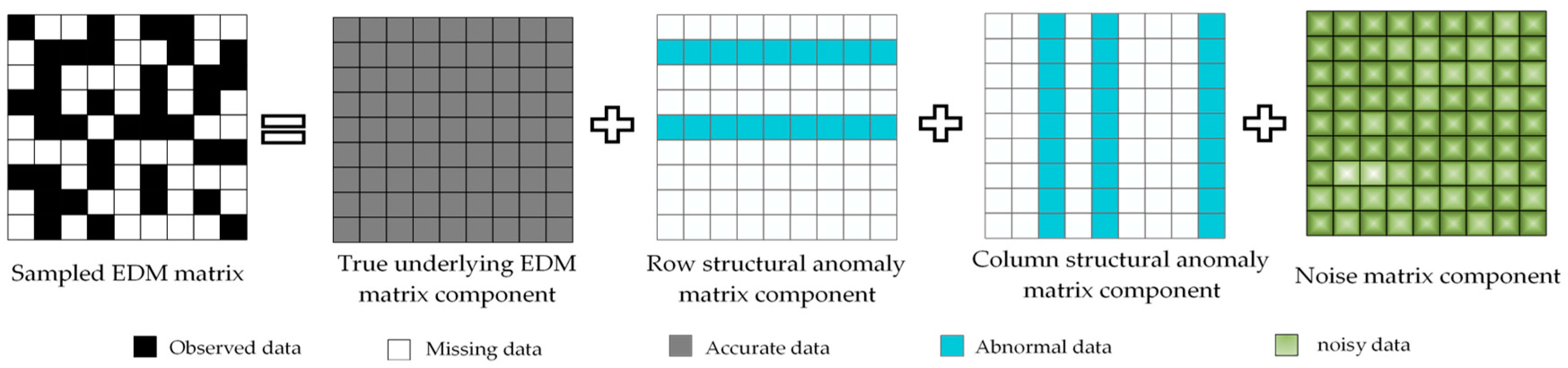
- A Robust -norm Regularized Matrix Decomposition (RRMD) model is proposed to jointly estimate the missing range measurements and detect the node anomaly, which takes advantage of the potential relationship between two tasks which could help each other to achieve more accurate performance.
- The MoG distribution is employed to fit the unknown complex noise, which allows the proposed RRMD model to adaptively handle a wider range of noise beyond the existing methods. Meanwhile, an efficient optimization algorithm is designed to solve the proposed RRMD model by adopting the popular EM method.
- A novel Anomaly-aware Node Localization (ANLoC) method is proposed based on the RRMD model, and extensive experiments verify the superior positioning performance of the ANLoC method in the coexistence of node anomaly and complex noise.
2. Related Work
2.1. Range-Based Node Localization
2.2. Low-Rank Matrix Decomposition
3. Preliminaries
3.1. Notations
3.2. Mathematical Foundation
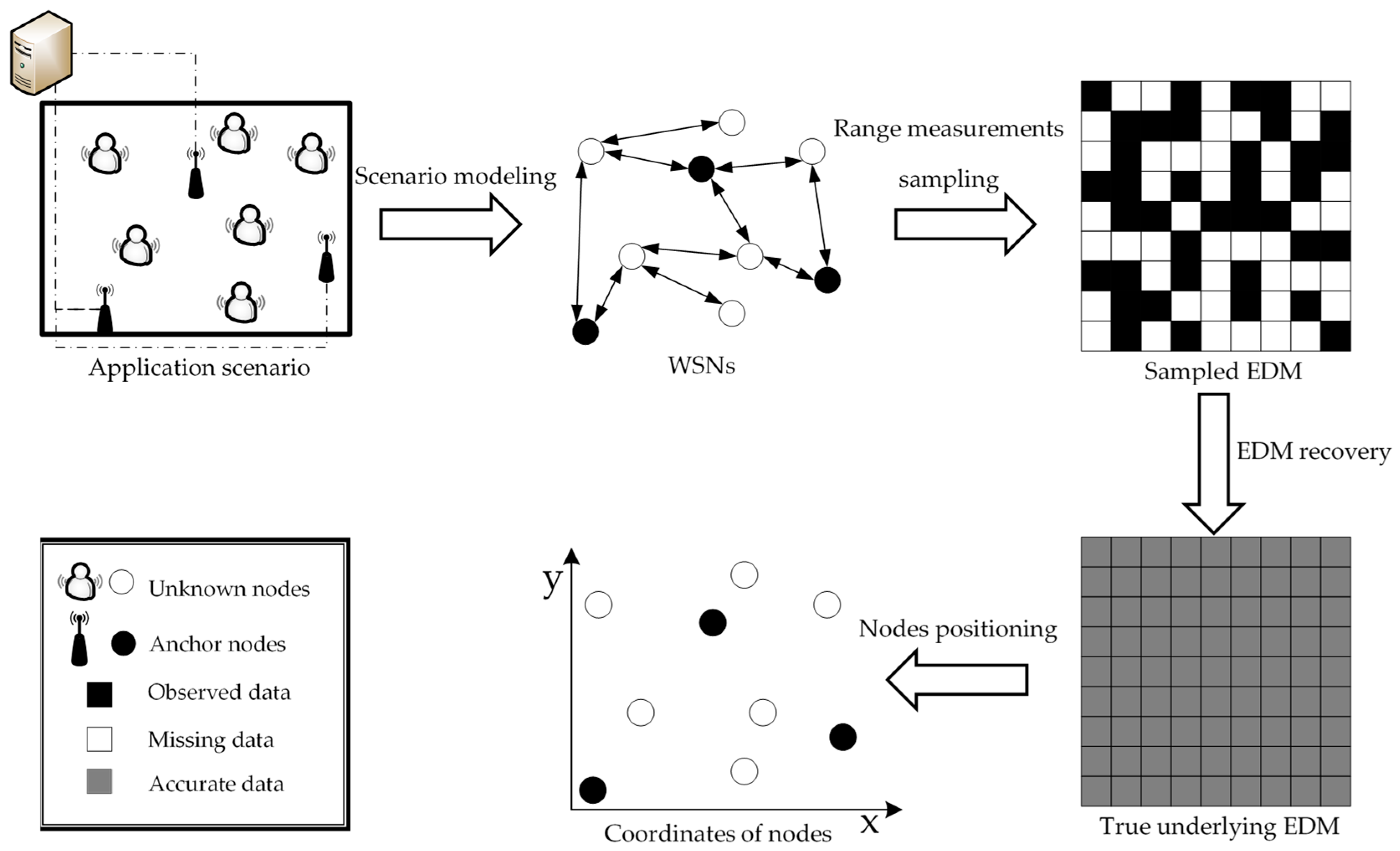
4. Anomaly-Aware Node Localization for WSNs
4.1. Euclidean Distance Matrix Completion
4.1.1. Problem Description and RRMD Model Construction
4.1.2. Optimizing RRMD via Expectation Maximization Method
| Algorithm 1. Proposed Robust -norm Regularized Matrix Decomposition (RRMD) Algorithm |
| Input: The sampled EDM matrix , the index set , the parameters , and threshold , the initial number of Gaussian components . |
| Output: The true underlying EDM matrix , the row structural anomaly and the column structural anomaly . |
| 1. Randomly initialize ; initialize to zero matrix; |
| 2. ; |
| 3. While not convergence do |
| 4. (E-step): update according to Equation (17); |
| 5. (M-step): update according to Equation (19) and Equation (20); |
| 6. (M-step): update according to optimize Equation (24); |
| 7. (M-step): update according to Equation (25); |
| 8. (M-step): update according to Equation (26); |
| 9. (Tuning ): Let and represent the number of -th and-th Gaussian component respectively. if , then let , , . Lastly, remove and from , respectively. |
| 10. ; |
| 11. End while |
| 12. . |
4.2. Anomaly-Aware Node Localization
| Algorithm 2. Anomaly-aware Node Localization (ANLoC) Algorithm |
| Input: The sampled EDM matrix , the index set , the parameters , and threshold , the initial number of Gaussian components . The coordinates of anchor nodes where denotes the number of anchor nodes. |
| Output: Coordinates of all unknown nodes . |
| 1. Calculate the true underlying EDM matrix by using Algorithm 1; |
| 2. Double centering the matrix : |
| , where and is identity matrix; |
| 3. Perform SVD decomposition on matrix : |
| ; |
| 4. Calculate relative coordinates: |
| where , , ; |
| 5. Calculate the coordinate transformation matrix : |
| ; |
| 6. Calculate and output coordinates of all unknown nodes: |
5. Performance Evaluation
5.1. Experimental Setting
5.2. Evaluation Metrics
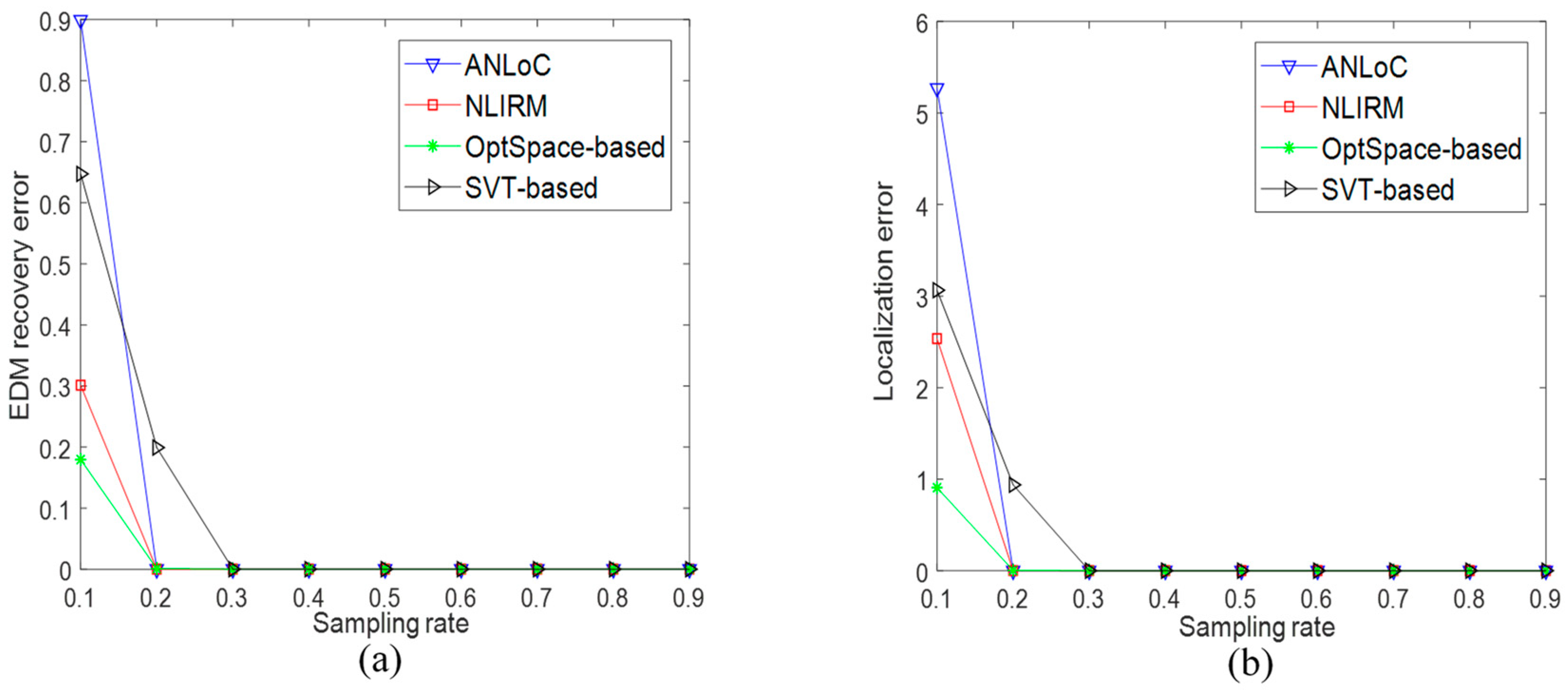
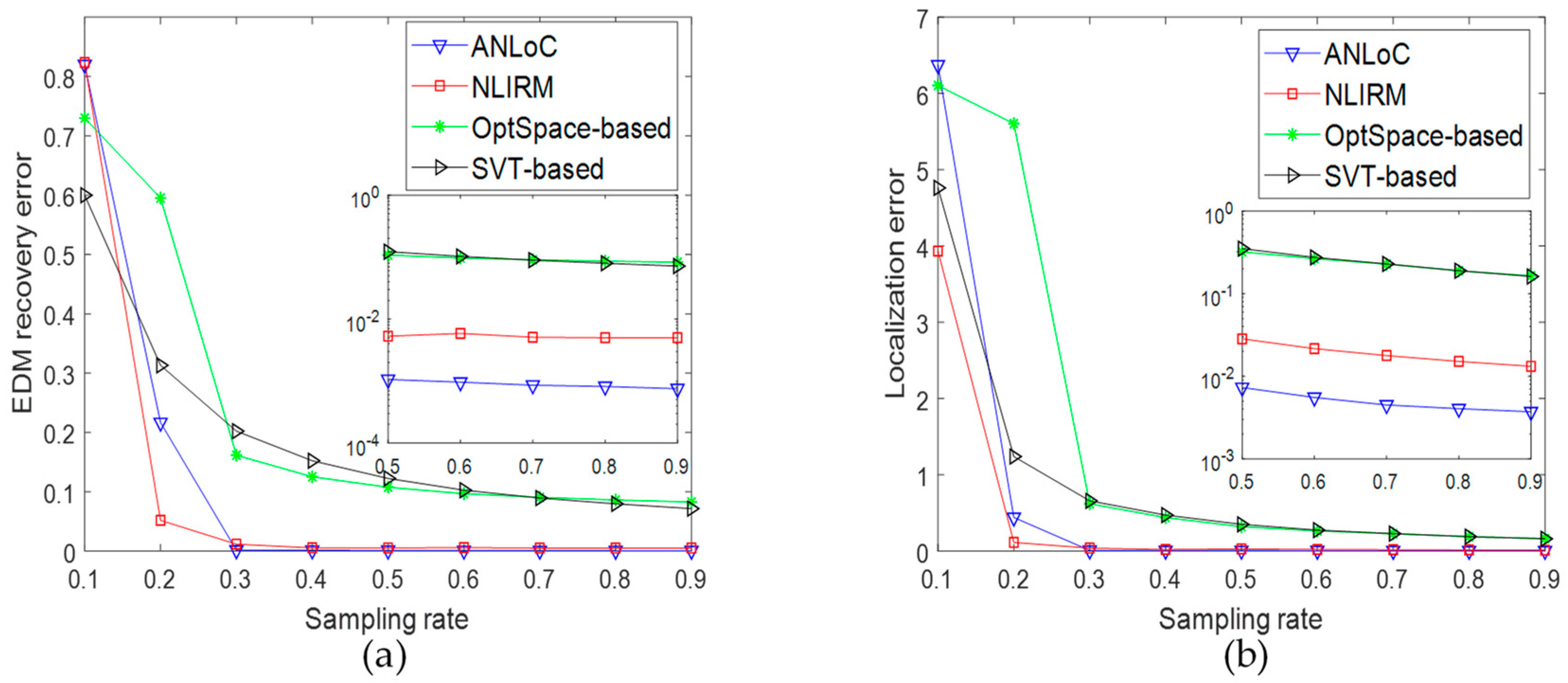
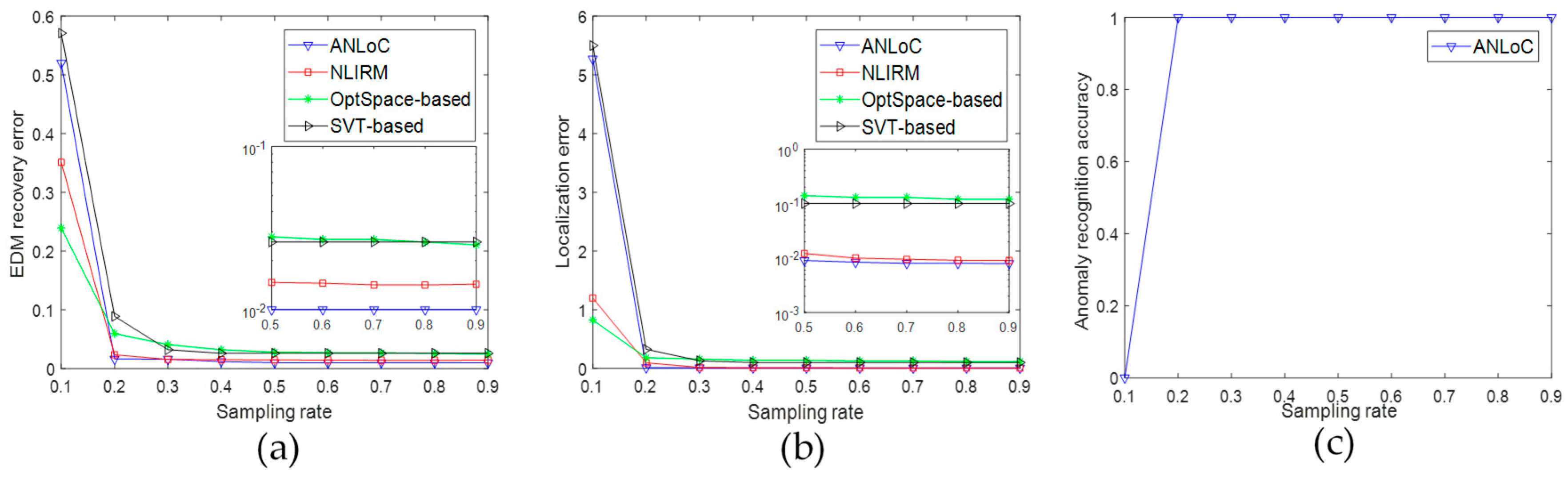
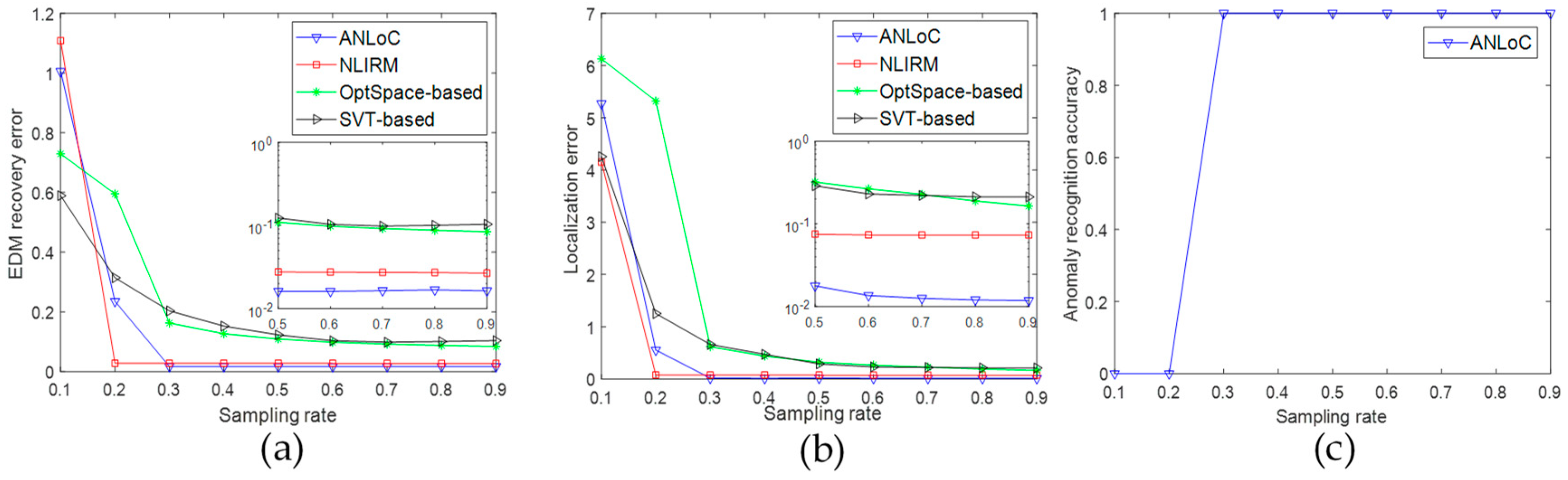
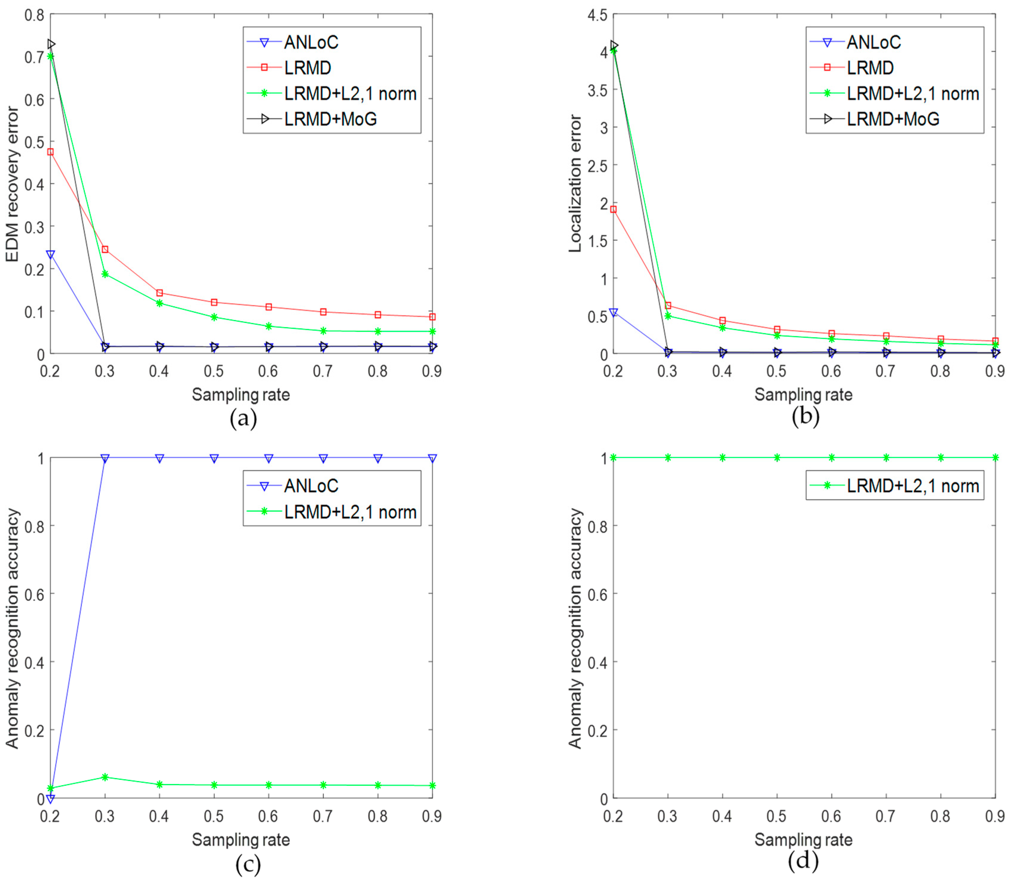
- EDM recovery error:where denotes the reconstructed matrix and is the ground truth matrix.
- Localization error:where denotes the coordinates calculated by Algorithm 2.
- Anomaly recognition accuracy:where and represent the row anomaly recognition accuracy and column anomaly recognition accuracy, respectively. Specifically, the is calculated bywhere represents the number of abnormal rows identified by the method proposed in this paper, indicates the number of correctly recognized rows in and represents the number of actual abnormal rows; the is calculated bywhere represents the number of abnormal columns identified by the method proposed in this paper, indicates the number of correctly recognized columns in and represents the number of actual abnormal columns.
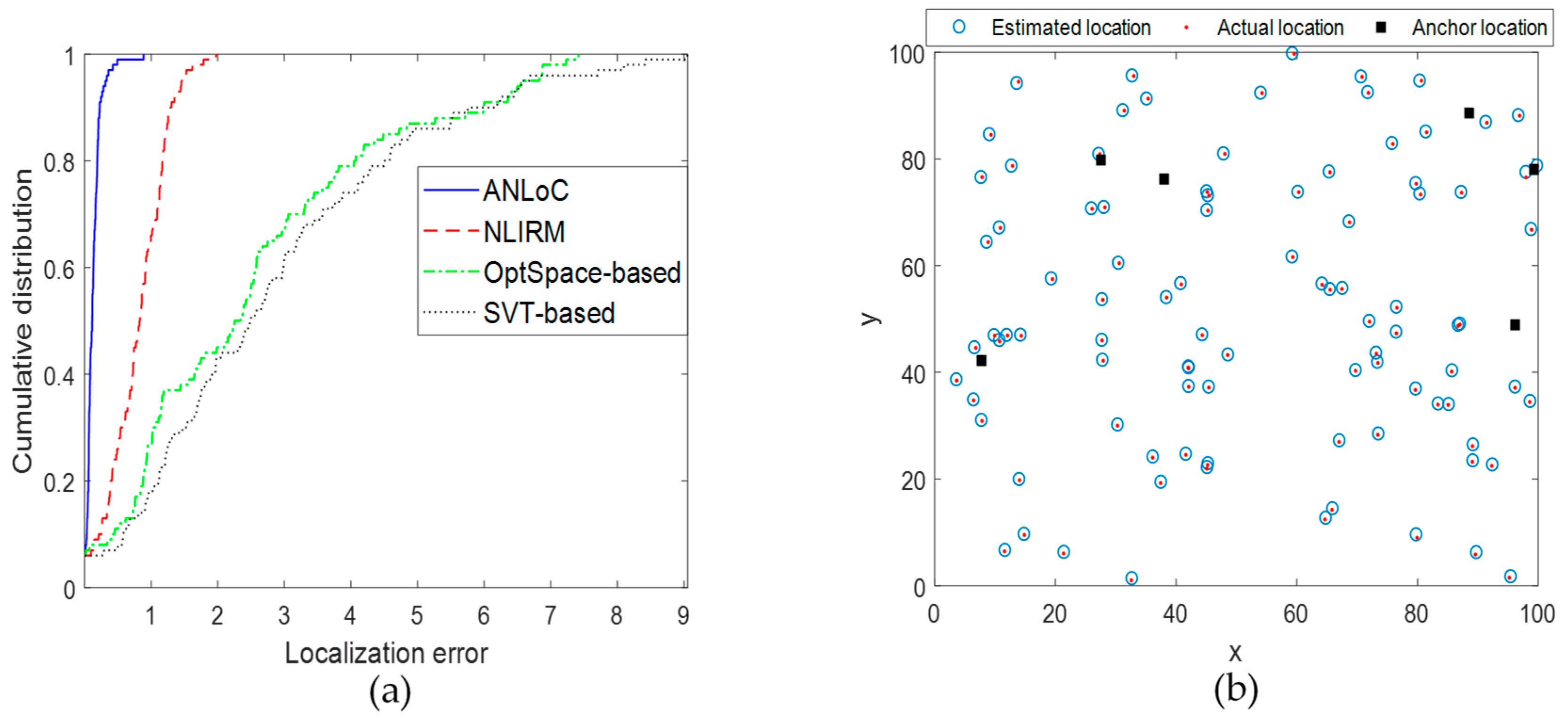
- Cumulative distribution of localization errors [21]:where defines the localization error of -th node, and denote the actual coordinates and the estimated coordinates, respectively.
5.3. Experimental Results
5.4. Effects of the Proposed Strategies
5.5. Localization for Large-Scale Scenario
6. Conclusions
Author Contributions
Funding
Conflicts of Interest
References
- Zheng, K.; Wang, H.; Li, H.; Xiang, W.; Lei, L.; Qiao, J.; Shen, X.S. Energy-efficient localization and tracking of mobile devices in wireless sensor networks. IEEE Trans. Veh. Technol. 2017, 66, 2714–2726. [Google Scholar] [CrossRef]
- Qian, H.; Fu, P.; Li, B.; Liu, J.; Yuan, X. A Novel Loss Recovery and Tracking Scheme for Maneuvering Target in Hybrid WSNs. Sensors 2018, 18, 341. [Google Scholar] [CrossRef] [PubMed]
- Zhu, H.; Xiao, F.; Sun, L.; Wang, R.; Yang, P. R-TTWD: Robust device-free through-the-wall detection of moving human with WiFi. IEEE J. Sel. Areas Commun. 2017, 35, 1090–1103. [Google Scholar] [CrossRef]
- Akyildiz, I.F.; Su, W.; Sankarasubramaniam, Y.; Cayirci, E. A survey on sensor networks. IEEE Commun. Mag. 2002, 40, 102–114. [Google Scholar] [CrossRef]
- Patwari, N.; Ash, J.N.; Kyperountas, S.; Hero, A.O.; Moses, R.L.; Correal, N.S. Locating the nodes: Cooperative localization in wireless sensor networks. IEEE Signal Processing Mag. 2005, 22, 54–69. [Google Scholar] [CrossRef]
- Xiao, F.; Sha, C.; Chen, L.; Sun, L.; Wang, R. Noise-tolerant localization from incomplete range measurements for wireless sensor networks. In Proceedings of the 2015 IEEE Conference on Computer Communications (INFOCOM), Hong Kong, China, 26–30 April 2015; pp. 2794–2802. [Google Scholar]
- Karbasi, A.; Oh, S. Robust localization from incomplete local information. IEEE/ACM Trans. Netw. 2013, 21, 1131–1144. [Google Scholar] [CrossRef]
- Xiao, F.; Liu, W.; Li, Z.; Chen, L.; Wang, R. Noise-tolerant wireless sensor networks localization via multinorms regularized matrix completion. IEEE Trans. Veh. Technol. 2018, 67, 2409–2419. [Google Scholar] [CrossRef]
- Maz’ya, V.; Schmidt, G. On approximate approximations using Gaussian kernels. IMA J. Numer. Anal. 1996, 16, 13–29. [Google Scholar] [CrossRef]
- Meng, D.; De La Torre, F. Robust matrix factorization with unknown noise. In Proceedings of the 2013 IEEE International Conference on Computer Vision, Sydney, NSW, Australia, 1–8 December 2013; pp. 1337–1344. [Google Scholar]
- Yao, J.; Cao, X.; Zhao, Q.; Meng, D.; Xu, Z. Robust subspace clustering via penalized mixture of Gaussians. Neurocomputing 2018, 278, 4–11. [Google Scholar] [CrossRef]
- Dempster, A.P.; Laird, N.M.; Rubin, D.B. Maximum likelihood from incomplete data via the EM algorithm. J. R. Stat. Soc. Ser. B 1977, 39, 1–38. [Google Scholar] [CrossRef]
- Shang, Y.; Ruml, W.; Zhang, Y.; Fromherz, M.P. Localization from mere connectivity. In Proceedings of the 4th ACM international symposium on Mobile ad hoc networking computing, Annapolis, MD, USA, 1–3 June 2003; pp. 201–212. [Google Scholar]
- Sheng, X.; Hu, Y.H. Maximum likelihood multiple-source localization using acoustic energy measurements with wireless sensor networks. IEEE Signal Processing Mag. 2005, 53, 44–53. [Google Scholar] [CrossRef]
- Tomic, S.; Beko, M.; Dinis, R. RSS-based localization in wireless sensor networks using convex relaxation: Noncooperative and cooperative schemes. IEEE Trans. Veh. Technol. 2015, 64, 2037–2050. [Google Scholar] [CrossRef]
- So, A.M.C.; Ye, Y. Theory of semidefinite programming for sensor network localization. Math. Program. 2007, 109, 367–384. [Google Scholar] [CrossRef]
- Shamsi, D.; Taheri, N.; Zhu, Z.; Ye, Y. Conditions for correct sensor network localization using SDP relaxation. In Discrete Geometry and Optimization; Springer: Heidelberg, Germany, 2013; pp. 279–301. [Google Scholar]
- Nguyen, T.L.N.; Shin, Y. Matrix completion optimization for localization in wireless sensor networks for intelligent IoT. Sensors 2016, 16, 722. [Google Scholar] [CrossRef] [PubMed]
- Sun, X.; Chen, T.; Li, W.; Zheng, M. Perfomance research of improved mds-map algorithm in wireless sensor networks localization. In Proceedings of the 2012 International Conference on Computer Science and Electronics Engineering (ICCSEE), Hangzhou, China, 23–25 March 2012; pp. 587–590. [Google Scholar]
- Feng, C.; Valaee, S.; Au, W.S.A.; Tan, Z. Localization of wireless sensors via nuclear norm for rank minimization. In Proceedings of the 2010 IEEE Global Telecommunications Conference GLOBECOM 2010, Miami, FL, USA, 6–10 December 2010; pp. 1–5. [Google Scholar]
- Liu, C.; Shan, H.; Wang, B. Wireless Sensor Network Localization via Matrix Completion Based on Bregman Divergence. Sensors 2018, 18, 2974. [Google Scholar] [CrossRef] [PubMed]
- Lee, D.D.; Seung, H.S. Algorithms for non-negative matrix factorization. Adv. Neural Inf. Processing Syst. 2001, 556–562. [Google Scholar]
- Sun, R.; Luo, Z.Q. Guaranteed matrix completion via non-convex factorization. IEEE Trans. Inf. Theory 2016, 62, 6535–6579. [Google Scholar] [CrossRef]
- Koren, Y.; Bell, R.; Volinsky, C. Matrix factorization techniques for recommender systems. Computer 2009, 8, 30–37. [Google Scholar] [CrossRef]
- Liu, H.; Wu, Z.; Li, X.; Cai, D.; Huang, T.S. Constrained nonnegative matrix factorization for image representation. IEEE Trans. Pattern Anal. Mach. Intell. 2012, 34, 1299–1311. [Google Scholar] [CrossRef] [PubMed]
- Parikh, N.; Boyd, S. Proximal algorithms. Found. Trends® Optim. 2014, 1, 127–239. [Google Scholar] [CrossRef]
- Chen, L.; Zhang, H.; Lu, J.; Thung, K.; Aibaidula, A.; Liu, L.; Chen, S.; Jin, L.; Wu, J.; Wang, Q.; Zhou, L.; Shen, D. Multi-label nonlinear matrix completion with transductive multi-task feature selection for joint MGMT and IDH1 status prediction of patient with high-grade gliomas. IEEE Trans. Med. Imaging 2018, 37, 1775–1787. [Google Scholar] [CrossRef] [PubMed]
- Armijo, L. Minimization of functions having Lipschitz continuous first partial derivatives. Pac. J. Math. 1966, 16, 1–3. [Google Scholar] [CrossRef]
- Chen, L.; Yang, G.; Chen, Z.; Xiao, F.; Shi, J. Correlation consistency constrained matrix completion for web service tag refinemen. Neural Comput. Appl. 2015, 26, 101–110. [Google Scholar] [CrossRef]
- De La Torre, F.; Black, M.J. A framework for robust subspace learning. Int. J. Comput. Vis. 2003, 54, 117–142. [Google Scholar] [CrossRef]
- Srebro, N.; Jaakkola, T. Weighted low-rank approximations. In Proceedings of the 20th International Conference on Machine Learning (ICML-03), Washington, DC, USA, 21–24 August 2003; pp. 720–727. [Google Scholar]
- Buchanan, A.M.; Fitzgibbon, A.W. Damped newton algorithms for matrix factorization with missing data. In Proceedings of the 2005 Computer Vision and Pattern Recognition, San Diego, CA, USA, 20–26 June 2005; pp. 316–322. [Google Scholar]
- Keshavan, R.H.; Montanari, A.; Oh, S. Matrix completion from a few entries. IEEE Trans. Inf. Theory 2010, 56, 2980–2998. [Google Scholar] [CrossRef]


| Name | Value | Name | Value |
|---|---|---|---|
| Size of experimental scenario | Gaussian noise 1 | Mean 0, variance 100 | |
| Number of sensor nodes | 100 | Gaussian noise 2 | Mean 0, variance 50 |
| Number of anchors | 6 | Range of sparse noise | |
| Range of row anomaly | Range of column anomaly |
© 2019 by the authors. Licensee MDPI, Basel, Switzerland. This article is an open access article distributed under the terms and conditions of the Creative Commons Attribution (CC BY) license (http://creativecommons.org/licenses/by/4.0/).
Share and Cite
Xu, P.; Cui, T.; Chen, L. ANLoC: An Anomaly-Aware Node Localization Algorithm for WSNs in Complex Environments. Sensors 2019, 19, 1912. https://doi.org/10.3390/s19081912
Xu P, Cui T, Chen L. ANLoC: An Anomaly-Aware Node Localization Algorithm for WSNs in Complex Environments. Sensors. 2019; 19(8):1912. https://doi.org/10.3390/s19081912
Chicago/Turabian StyleXu, Pengfei, Tianhao Cui, and Lei Chen. 2019. "ANLoC: An Anomaly-Aware Node Localization Algorithm for WSNs in Complex Environments" Sensors 19, no. 8: 1912. https://doi.org/10.3390/s19081912
APA StyleXu, P., Cui, T., & Chen, L. (2019). ANLoC: An Anomaly-Aware Node Localization Algorithm for WSNs in Complex Environments. Sensors, 19(8), 1912. https://doi.org/10.3390/s19081912