A 3D Coverage Algorithm Based on Complex Surfaces for UAVs in Wireless Multimedia Sensor Networks


Abstract
:1. Introduction
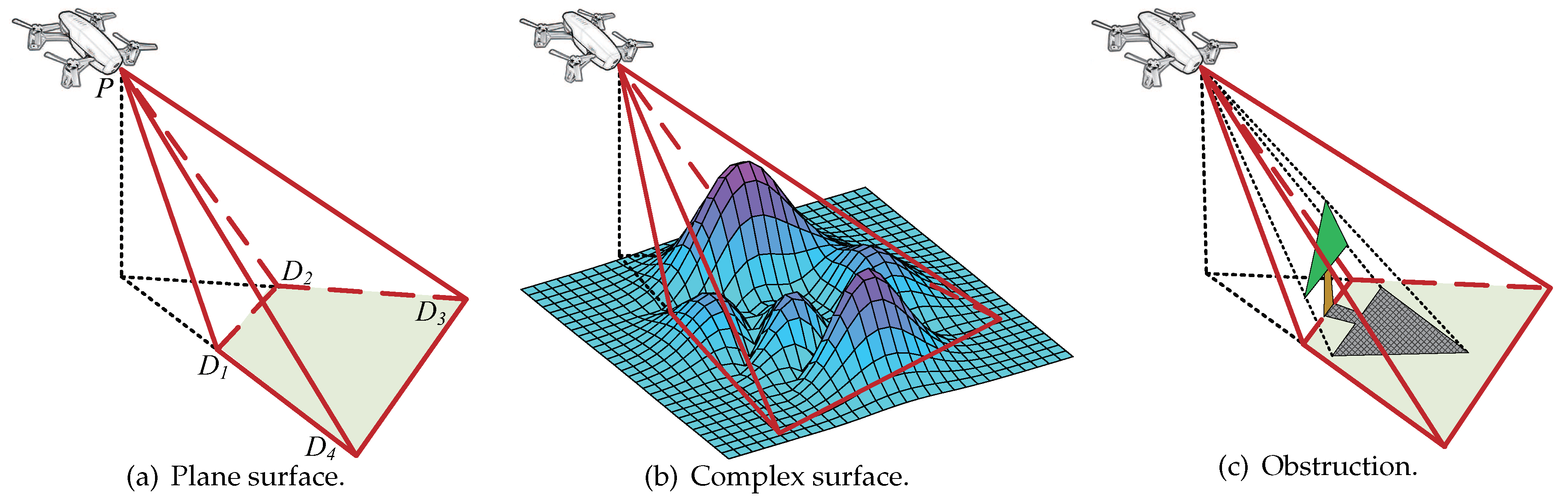
- A 3D complex surface sensing model is proposed that reflects the real sensing area of the camera sensors. The model extracts the complex surface-related information based on a set of rules that satisfy the precision demands and efficiency
- Considering the fact that the monitoring area may be obstructed by physical barriers, such as hills or buildings, we propose a coverage-based map to help solve this problem. This model provides an achievable shade rule which quantifies the actual sensing area for each sensor.
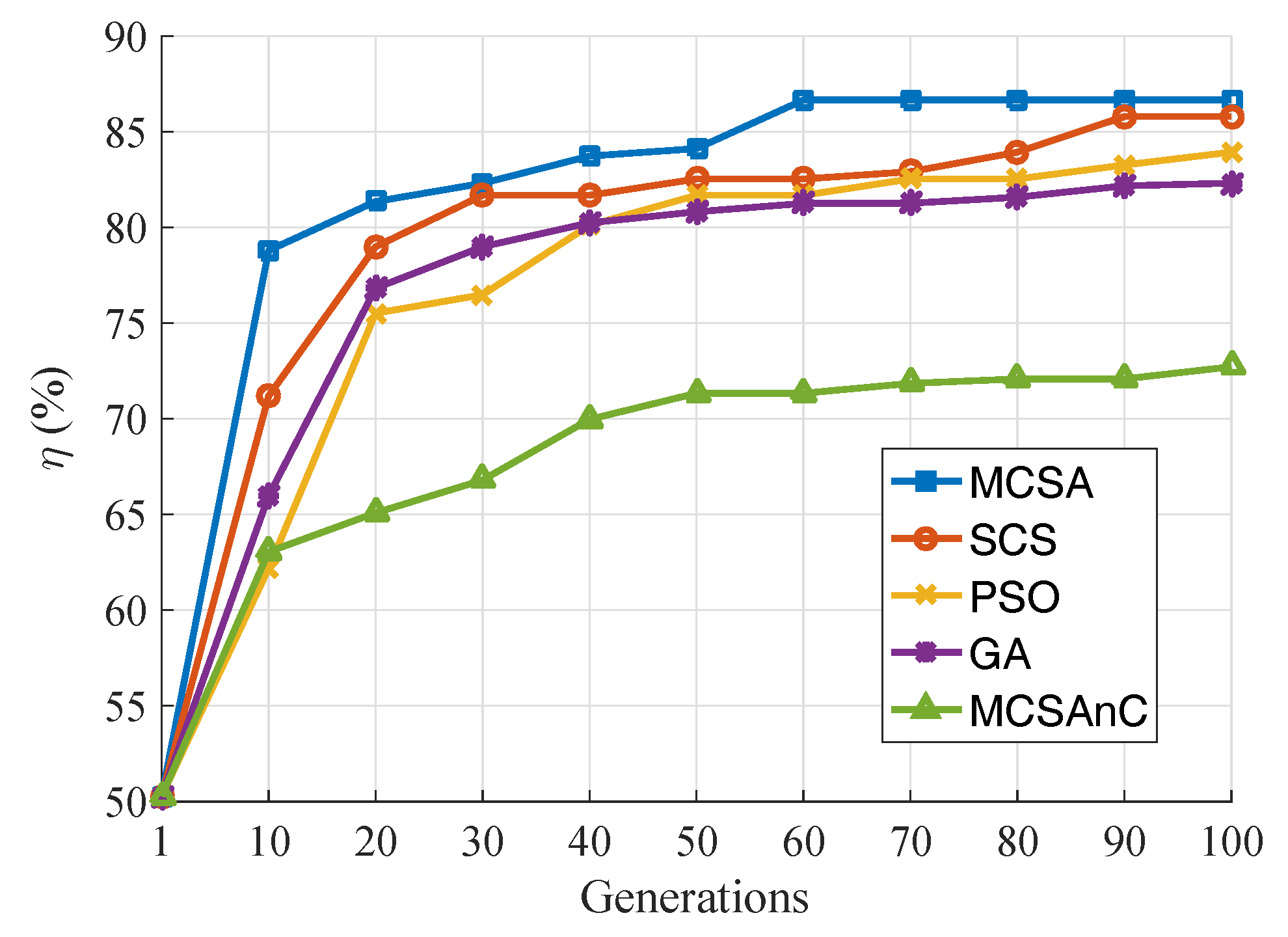
- We propose a modified cuckoo search algorithm (MCSA) to compute the coverage area of the complex surface based on the survival of the fittest, dynamic discovery probability, and the self-adaptation strategy of rotation. Based on different parameter settings, our sensing models can be used for practical applications. The probabilistic algorithm is also adequate for the deterministic and stochastic deployment of WMSN.
2. Motivation
2.1. Benefits of Sensing Deployment
2.2. 3D Coverage Algorithm on Complex Surfaces
2.3. Challenges
- The 3D sensing model for the calculation of the coverage area is complex. On the basis of different backgrounds, we need to analyze the sensing model from different directions. Building a 3D sensing model for every sensor is not an easy task. Even though the calculation of the sensing model and surface function of different terrains will produce accurate results, there is still a significant computational problem because the directions of the sensors are not fixed
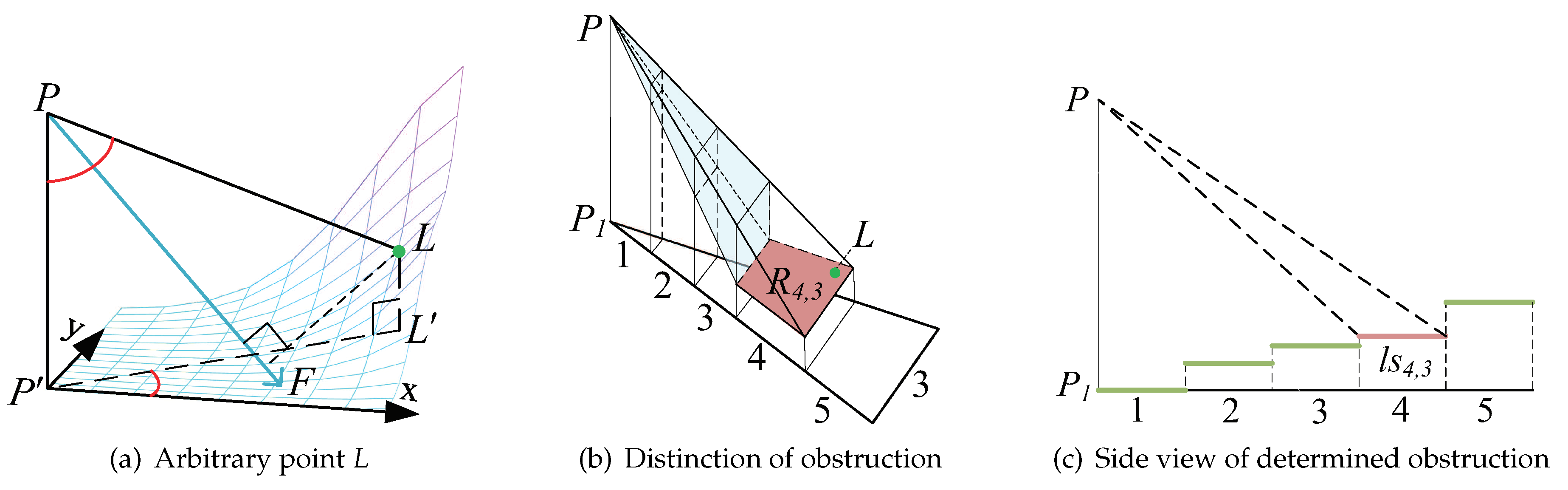
- Any obstruction on the complex surface will reduce the monitoring efficiency. In a real WMSN system, the relations among sensor, obstruction, and raw complex surface data, are always intricate and expensive to manipulate and analyze. Moreover, obstructions impose different impacts because of the different heights and distances to the sensor
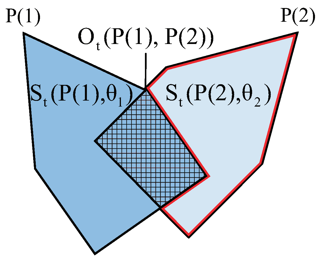
- Optimizing the directions of multiple sensors is not an easy task. Rotating any of the sensors may overlap the coverage areas from other sensors or may miss the monitoring of key areas, thereby influencing the monitoring outcome
3. Model Design
3.1. 3D Sensing Model
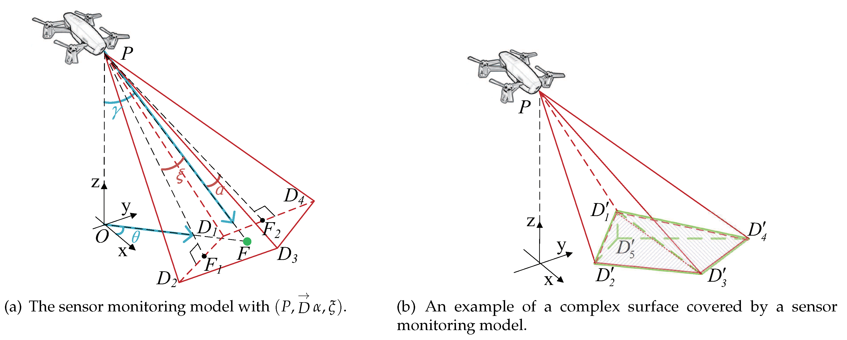
3.1.1. Sensor Monitoring Model
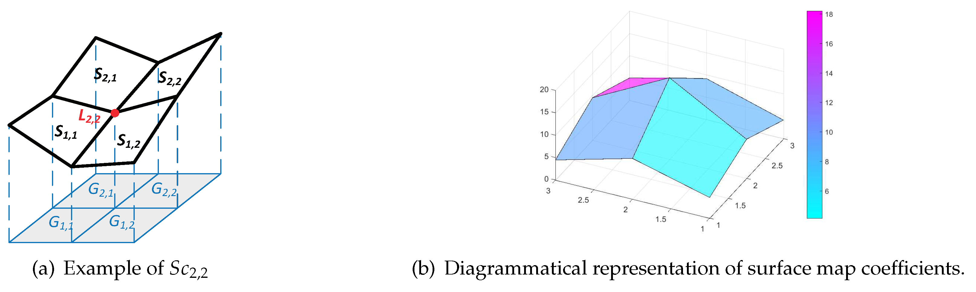
3.1.2. Surface-map Calculation
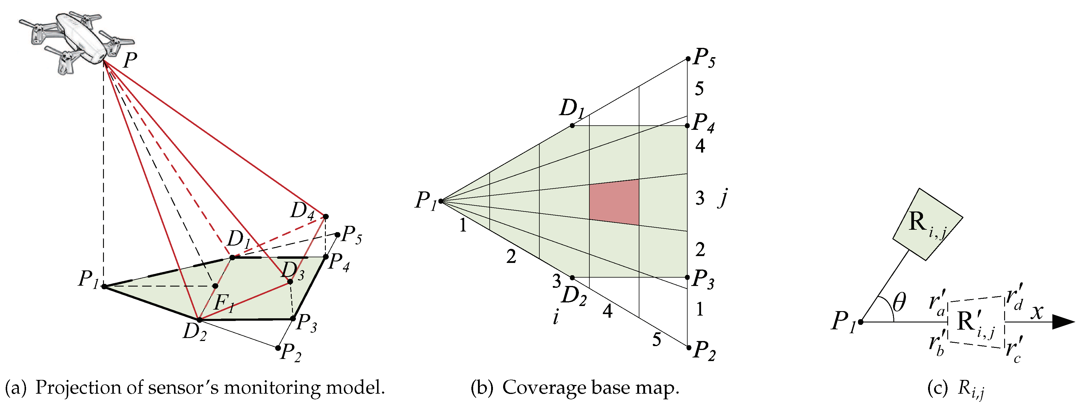
3.2. Coverage Base Map
3.3. Determination of Coverage
4. Modified Cuckoo Search Algorithm
4.1. Cuckoo Search for WMSN
| Algorithm 1: MSCA |
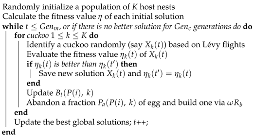 |
4.2. Survival of the Fittest
4.3. Dynamic Discovery Probability
4.4. Self-adaptation Rotation Strategy
5. Evaluation
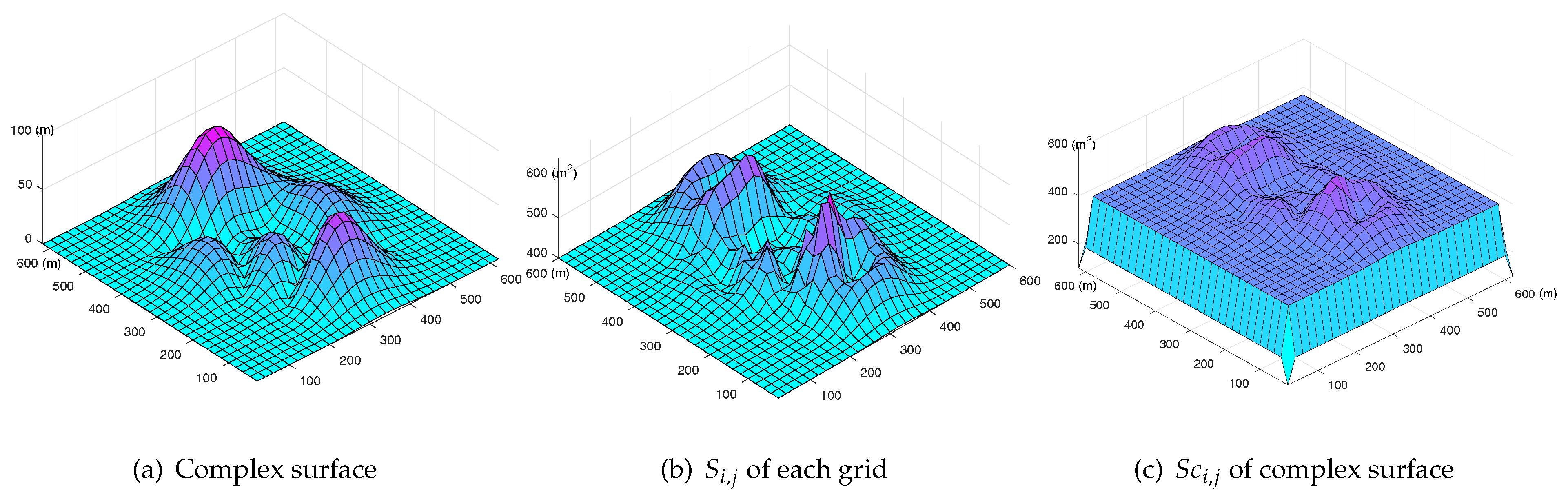
5.1. Surface Map
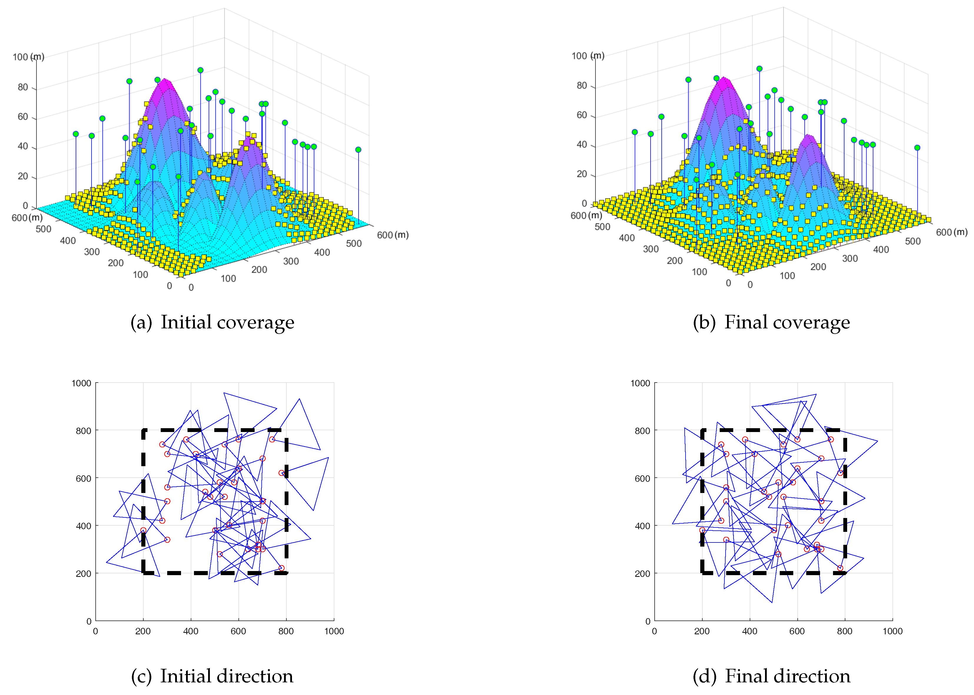
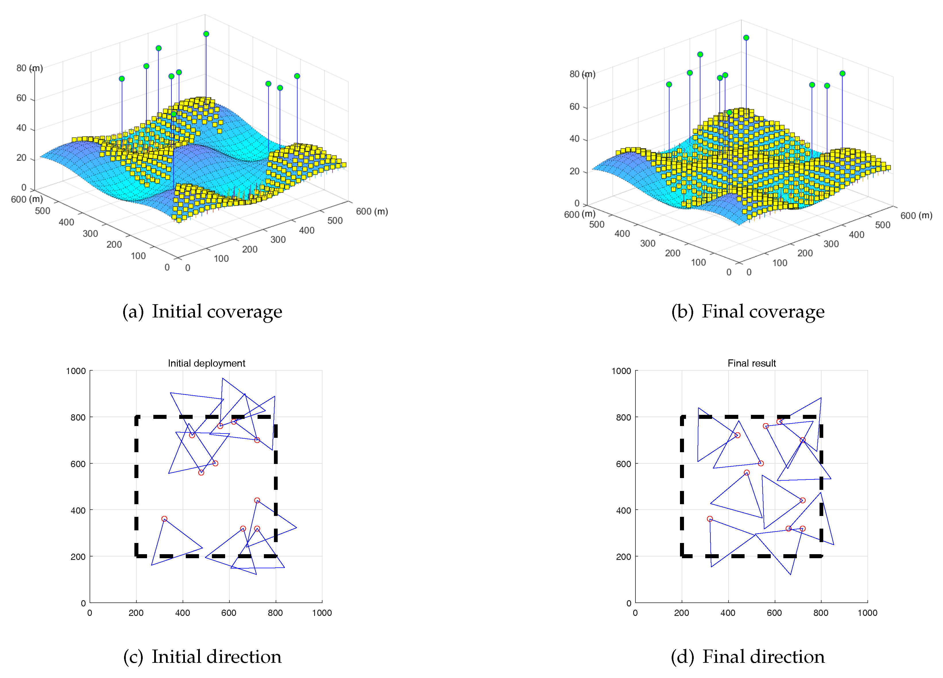
5.2. 3D Coverage on Complex Surfaces
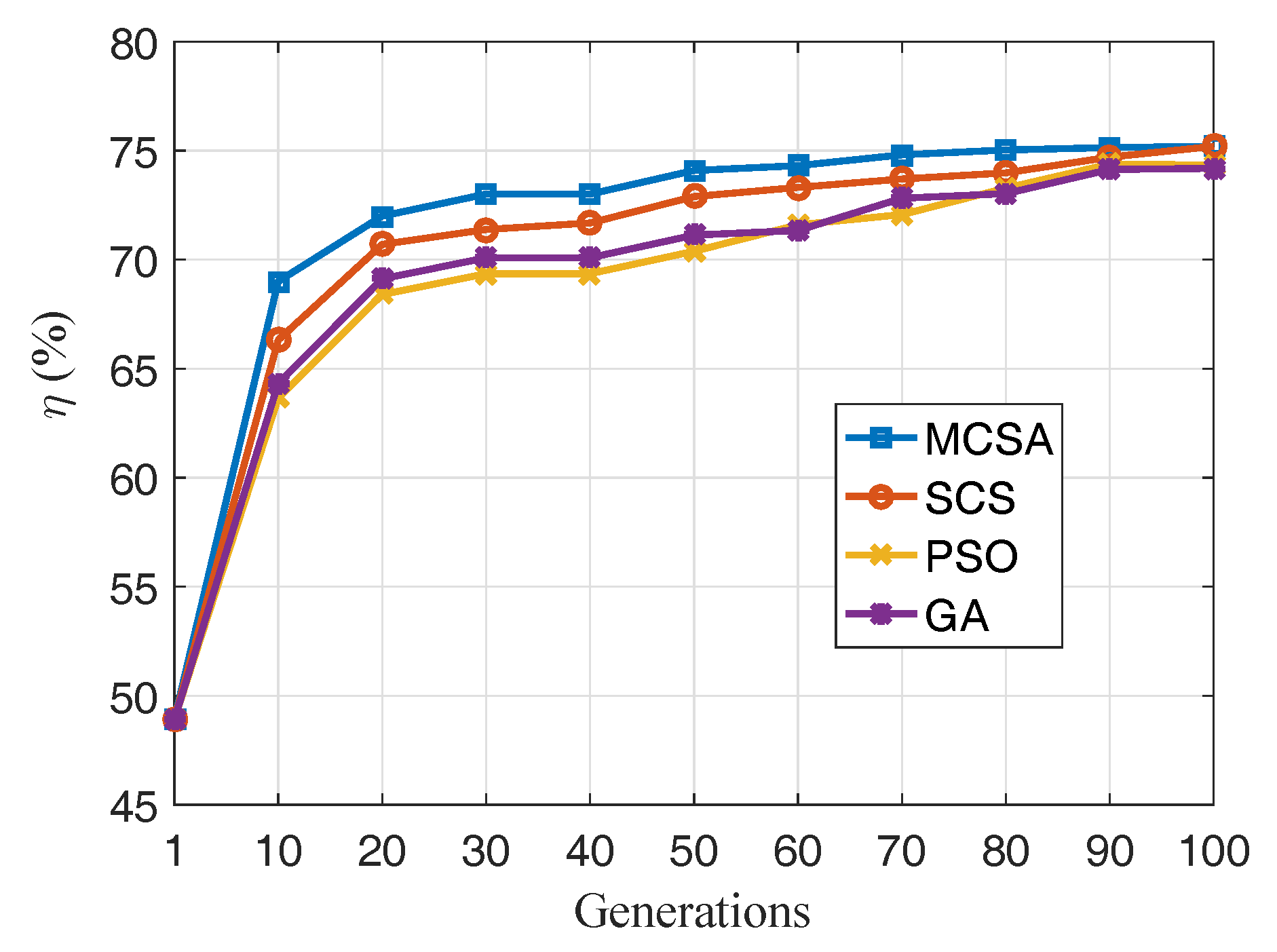
5.3. Effectiveness of MSCA
6. Related Studies
7. Conclusions
Author Contributions
Acknowledgments
Conflicts of Interest
Appendix A
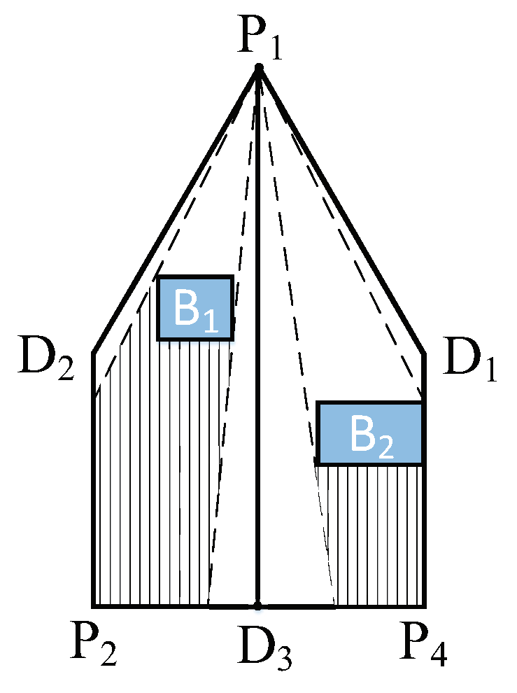
- , and :If we assume that the coordinate of the sensor P is , we can determine the XOY coordinates of , and on the plane of as follows.
- , , , :As shown in Figure 4c, the turning points of the on the X–axis are indicated by , , , on the plane of . Utilizing a similar triangular methodology, we can calculate these coordinates, as follows.
- , , , :Considering the angle of the sensor, all the coordinates of of are calculated based on an anticlockwise rotation by with respect to the positive direction of the X–axis using the rotation matrix, as follows.where represents the XOY coordinates of , , , and represents the XOY coordinates of , , , .
- , , and :The XOY coordinate of , , , and , can be calculated as follows.According to Equation (5), we can calculate that
References
- Sen, J. A survey on wireless sensor network security. arXiv 2010, arXiv:1011.1529. [Google Scholar]
- Sakthidharan, G.; Chitra, S. A survey on wireless sensor network: An application perspective. In Proceedings of the 2012 International Conference on Computer Communication and Informatics, Coimbatore, India, 10–12 January 2012; pp. 1–5. [Google Scholar]
- Si, P.; Wu, C.; Zhang, Y.; Jia, Z.; Ji, P.; Chu, H. Barrier coverage for 3d camera sensor networks. Sensors 2017, 17, 1771. [Google Scholar] [CrossRef]
- Yan, T.; He, T.; Stankovic, J.A. Differentiated surveillance for sensor networks. In Proceedings of the 1st International Conference on Embedded Networked Sensor Systems, Los Angeles, CA, USA, 5–7 November 2003; pp. 51–62. [Google Scholar]
- Ammari, H.M.; Das, S.K. Critical density for coverage and connectivity in three-dimensional wireless sensor networks using continuum percolation. IEEE Trans. Parallel Distrib. Syst. 2009, 20, 872–885. [Google Scholar] [CrossRef]
- Zhu, C.; Zheng, C.; Shu, L.; Han, G. A survey on coverage and connectivity issues in wireless sensor networks. J. Netw. Comput. Appl. 2012, 35, 619–632. [Google Scholar] [CrossRef]
- Han, R.; Yang, W.; Zhang, L. Achieving Crossed Strong Barrier Coverage in Wireless Sensor Network. Sensors 2018, 18, 534. [Google Scholar] [CrossRef]
- Kim, H.; Oh, H.; Bellavista, P.; Ben-Othman, J. Constructing Event-driven Partial Barriers with Resilience in Wireless Mobile Sensor Networks. J. Netw. Comput. Appl. 2017, 82, 77–92. [Google Scholar] [CrossRef]
- Zou, Y.; Chakrabarty, K. Sensor deployment and target localization based on virtual forces. In Proceedings of the Twenty-second Annual Joint Conference of the IEEE Computer and Communications Societies (IEEE INFOCOM 2003), San Francisco, CA, USA, 30 March–3 April 2003; pp. 1293–1303. [Google Scholar]
- Zhuang, Y.; Wu, C.; Zhang, Y.; Jia, Z. Compound event barrier coverage algorithm based on environment Pareto dominated selection strategy in multi-constraints sensor networks. IEEE Access 2017, 5, 10150–10160. [Google Scholar] [CrossRef]
- Zhuang, Y.; Wu, C.; Zhang, Y. Non-Preference Bi-Objective Compound Event Barrier Coverage Algorithm in 3-D Sensor Networks. IEEE Access 2018, 6, 34086–34097. [Google Scholar] [CrossRef]
- Si, P.; Wu, C.; Zhang, Y.; Chu, H.; Teng, H. Probabilistic coverage in directional sensor networks. Wirel. Netw. 2017. [Google Scholar] [CrossRef]
- Si, P.; Wu, C.; Zhang, Y.; Ji, P.; Jia, Z. 3D sensing model based on ROI for camera sensor networks. In Proceedings of the 36th Chinese Control Conference (CCC), Dalian, China, 26–28 July 2017; pp. 8940–8945. [Google Scholar]
- Akbarzadeh, V.; Lévesque, J.C.; Gagné, C.; Parizeau, M. Efficient sensor placement optimization using gradient descent and probabilistic coverage. Sensors 2014, 14, 15525–15552. [Google Scholar] [CrossRef] [PubMed]
- Xiao, F.; Wang, R.C.; Sun, L.J.; Weng, J.Y. Coverage-enhancing algorithm for wireless multi-media sensor networks based on three-dimensional perception. Acta Electron. Sin. 2012, 40, 167–172. [Google Scholar]
- Jin, M.; Rong, G.; Wu, H.; Shuai, L.; Guo, X. Optimal surface deployment problem in wireless sensor networks. In Proceedings of the 31st Annual IEEE International Conference on Computer Communications (IEEE INFOCOM 2012), Orlando, FL, USA, 25–30 March 2012; pp. 2345–2353. [Google Scholar]
- Haines, E. Point in polygon strategies. In Graphics Gems IV; Heckbert, P., Ed.; Academic Press Professional Inc.: San Diego, CA, USA, 1994; pp. 24–26. [Google Scholar]
- Goldman, R. Intersection of two lines in three-space. In Graphics Gems IV; Academic Press Professional Inc.: San Diego, CA, USA, 1990. [Google Scholar]
- Yang, X.S.; Deb, S. Cuckoo search via Lévy flights. In Proceedings of the 2009 World Congress on Nature & Biologically Inspired Computing (NaBIC), Coimbatore, India, 9–11 December 2009; pp. 210–214. [Google Scholar]
- Wang, H.; Wang, W.; Sun, H.; Cui, Z.; Rahnamayan, S.; Zeng, S. A new cuckoo search algorithm with hybrid strategies for flow shop scheduling problems. Soft Comput. 2017, 21, 4297–4307. [Google Scholar] [CrossRef]
- Cheng, J.; Xia, L. An effective Cuckoo search algorithm for node localization in wireless sensor network. Sensors 2016, 16, 1390. [Google Scholar] [CrossRef] [PubMed]
- Yang, B.; Miao, J.; Fan, Z.; Long, J.; Liu, X. Modified cuckoo search algorithm for the optimal placement of actuators problem. Appl. Soft Comput. 2018, 67, 48–60. [Google Scholar] [CrossRef]
- Winfree, R. Cuckoos, cowbirds and the persistence of brood parasitism. Trends Ecol. Evol. 1999, 14, 338–343. [Google Scholar] [CrossRef]
- Zhao, K.; Jurdak, R.; Liu, J.; Westcott, D.; Kusy, B.; Parry, H.; Sommer, P.; Mckeown, A. Optimal Lévy-flight foraging in a finite landscape. J. R. Soc. Interface 2015, 12, 20141158. [Google Scholar] [CrossRef] [PubMed]
- Zhao, M.C.; Lei, J.; Wu, M.Y.; Liu, Y.; Shu, W. Surface coverage in wireless sensor networks. In Proceedings of the 28th IEEE International Conference on Computer Communications (IEEE INFOCOM), Rio de Janeiro, Brazil, 19–25 April 2009; pp. 109–117. [Google Scholar]
- Liu, L.; Ma, H. On Coverage of Wireless Sensor Networks for Rolling Terrains. IEEE Trans. Parallel Distrib. Syst. 2011, 23, 118–125. [Google Scholar] [CrossRef]
- Tao, D.; Ma, H.; Liu, L. Coverage-enhancing algorithm for directional sensor networks. In Proceedings of the Second International Conference on Mobile Ad-Hoc and Sensor Networks, Hong Kong, China, 13–15 December 2006; pp. 256–267. [Google Scholar]
- Cheng, W.; Li, S.; Liao, X.; Changxiang, S.; Chen, H. Maximal coverage scheduling in randomly deployed directional sensor networks. In Proceedings of the 2007 International Conference on Parallel Processing Workshops (ICPPW 2007), Xi’an, China, 10–14 September 2007; p. 68. [Google Scholar]
- Heo, N.; Varshney, P.K. Energy-efficient deployment of intelligent mobile sensor networks. IEEE Trans. Syst. Man Cybern. Part A Syst. Hum. 2005, 35, 78–92. [Google Scholar] [CrossRef]
- Ma, H.; Zhang, X.; Ming, A. A coverage-enhancing method for 3D directional sensor networks. In Proceedings of the 28th IEEE International Conference on Computer Communications (IEEE INFOCOM), Rio de Janeiro, Brazil, 19–25 April 2009; pp. 2791–2795. [Google Scholar]
- Cai, Y.; Lou, W.; Li, M.; Li, X.Y. Target-oriented scheduling in directional sensor networks. In Proceedings of the 26th IEEE International Conference on Computer Communications (IEEE INFOCOM), Anchorage, AK, USA, 6–12 May 2007; pp. 1550–1558. [Google Scholar]
- Huang, J.J.; Sun, L.J.; Wang, R.C.; Huang, H.P. Coverage-enhancing Algorithm for Three-dimensional Under-water Sensor Networks. J. Nanjing Univ. Posts Telecommun. 2013. (In Chinese) [Google Scholar]
- Bhuiyan, M.Z.A.; Wang, G.; Cao, J.; Wu, J. Deploying wireless sensor networks with fault-tolerance for structural health monitoring. IEEE Trans. Comput. 2015, 64, 382–395. [Google Scholar] [CrossRef]
- Xiang, Y.; Xuan, Z.; Tang, M.; Zhang, J.; Sun, M. 3D space detection and coverage of wireless sensor network based on spatial correlation. J. Netw. Comput. Appl. 2016, 61, 93–101. [Google Scholar] [CrossRef]


| Parameter Settings | Value |
|---|---|
| h of sensor | 50 m |
| of sensor | |
| of sensor | |
| of sensor | |
| Detection range | 200 m |
| Parameter Settings | Value |
|---|---|
| Sensor number N | 30 |
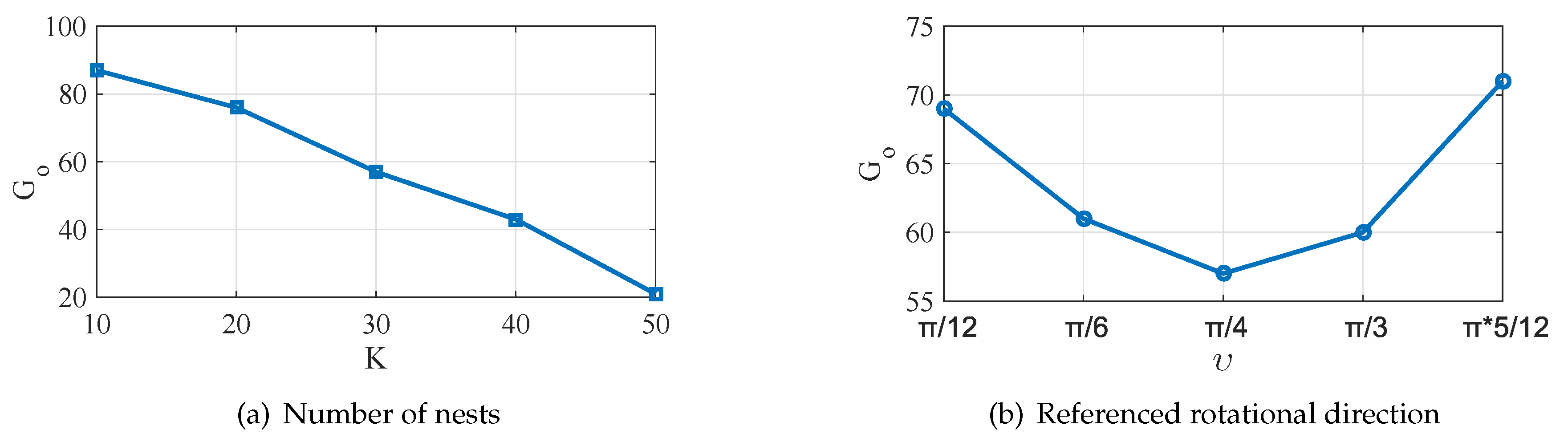
| Number of nest K | 20 |
| Basic discovery possibility | 0.25 |
| Referenced rotation direction | |
| 100 | |
| 10 |
| N | (Initial) | (Final) | Δ |
|---|---|---|---|
| 10 | 28.6 | 44.6 | 16% |
| 20 | 42.3 | 72.7 | 30.4% |
| 30 | 50.3 | 86.7 | 36.4% |
| 40 | 56.7 | 88.9 | 32.2% |
| 50 | 62.7 | 91.2 | 28.5% |
© 2019 by the authors. Licensee MDPI, Basel, Switzerland. This article is an open access article distributed under the terms and conditions of the Creative Commons Attribution (CC BY) license (http://creativecommons.org/licenses/by/4.0/).
Share and Cite
Ru, J.; Jia, Z.; Yang, Y.; Yu, X.; Wu, C.; Xu, M. A 3D Coverage Algorithm Based on Complex Surfaces for UAVs in Wireless Multimedia Sensor Networks. Sensors 2019, 19, 1902. https://doi.org/10.3390/s19081902
Ru J, Jia Z, Yang Y, Yu X, Wu C, Xu M. A 3D Coverage Algorithm Based on Complex Surfaces for UAVs in Wireless Multimedia Sensor Networks. Sensors. 2019; 19(8):1902. https://doi.org/10.3390/s19081902
Chicago/Turabian StyleRu, Jingyu, Zixi Jia, Yufang Yang, Xiaosheng Yu, Chengdong Wu, and Ming Xu. 2019. "A 3D Coverage Algorithm Based on Complex Surfaces for UAVs in Wireless Multimedia Sensor Networks" Sensors 19, no. 8: 1902. https://doi.org/10.3390/s19081902
APA StyleRu, J., Jia, Z., Yang, Y., Yu, X., Wu, C., & Xu, M. (2019). A 3D Coverage Algorithm Based on Complex Surfaces for UAVs in Wireless Multimedia Sensor Networks. Sensors, 19(8), 1902. https://doi.org/10.3390/s19081902