3.1. Transfer from Fault Diagnosis Model of Missing Data to the Model of Structurally Complete Data
Samples with incomplete structures may lose some information but contain other useful information. It is necessary to migrate them to a structurally complete fault diagnosis model. This section explains how to learn and extract fault features from a huge number of incomplete data and then migrate these extracted features from an incomplete data model to a structurally complete data model to enhance the fault diagnosis accuracy of the latter model. The fault diagnosis framework with missing data is shown in
Figure 2. The algorithm is as follows:
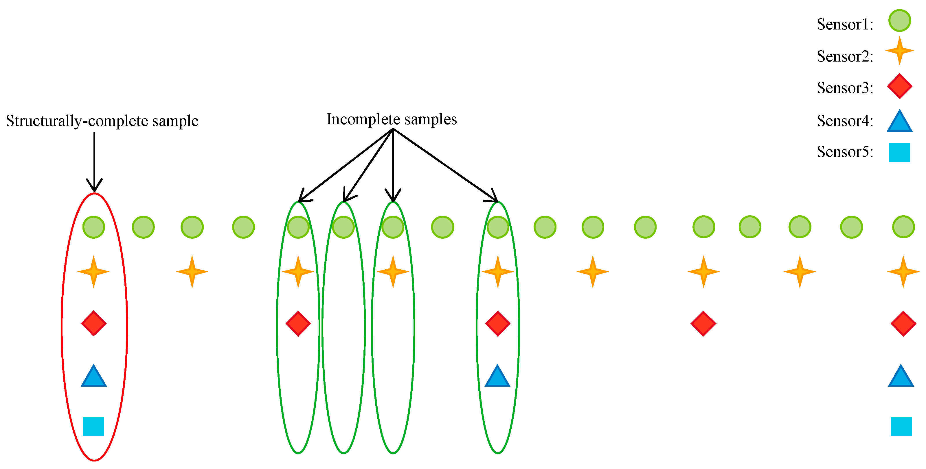
Step 1: Classifying samples based on missing data.
The sample set is divided into complete sample set
and incomplete sample set which is further classified into n categories
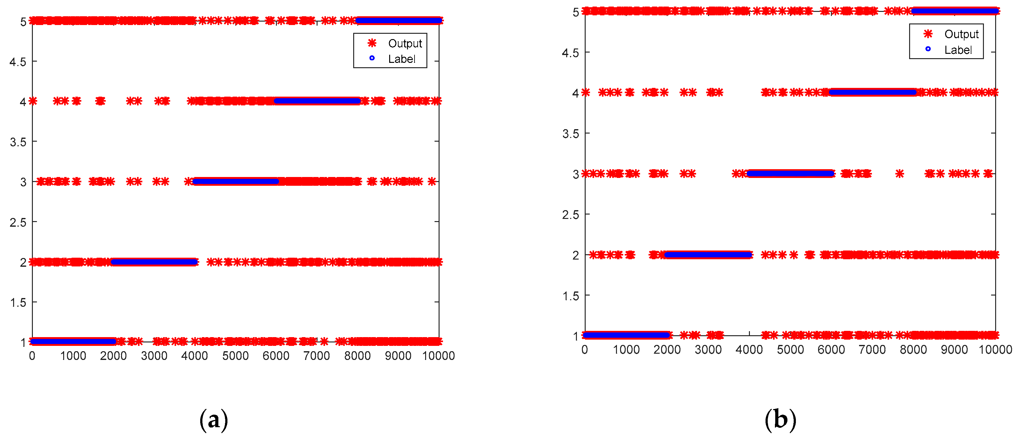
. Taking
Figure 1 as an example, the samples are divided into five categories, among which
is structurally complete sample set while
and
are structurally incomplete sample sets. When the sample value of sensor 5 is unavailable,
is used to represent the missing data set. When the sample values of sensor 4 and 5 are unavailable,
is used to represent the missing data set. When the sample values of sensor 3, 4 and 5 are unavailable,
is used to represent the missing data set. When the sample values of sensor 2, 3, 4 and 5 are unavailable,
is used to represent the missing data set. Supposing a structurally complete sample contains
P variables,
is 0 if the
pth variable of sample
is missing and 1 otherwise as indicated in Equation (13).
thus represents the missing state of
as shown in Equation (14).
If Equation (15) is true, it represents that sample is complete data while that Equation (16) is true means sample is missing data. If is true, sample and sample either are both complete data or belong to the same type of missing data as shown in Equation (17).
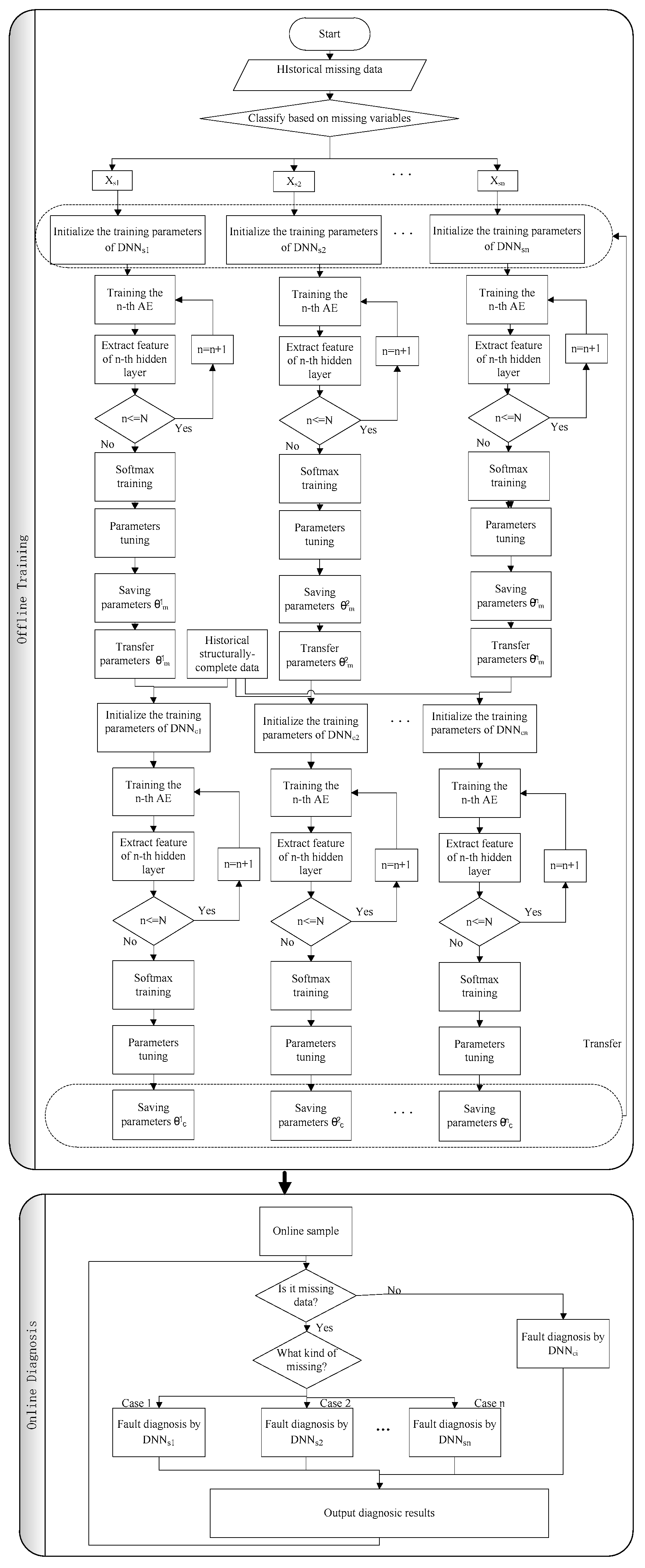
Step 2: Building fault diagnosis models for each type of missing data.
Let us take type i as an example and build its fault diagnosis model . is composed by stacking N autoencoders. are the neuron number of 1st, 2nd,…Nth hidden layers in , respectively. is the set of weight matrix and bias between input layer and hidden layer of in respectively and is initialized randomly. Then is the set of weight matrix and bias between hidden layer and output layer of in respectively and is randomly initialized as well. Likewise, we can build fault diagnosis models for missing data types 1, 2,…, n respectively.
Step 3: Training the models .
Taking as an example, is trained by historical missing data set and obtain the feature shown in . The model updates parameters and by Equations (5)–(8).
Step 4: Optimizing the models .
is used as input data to train Softmax model. Still taking as an example, is optimized by backpropagation algorithm and parameters are updated.
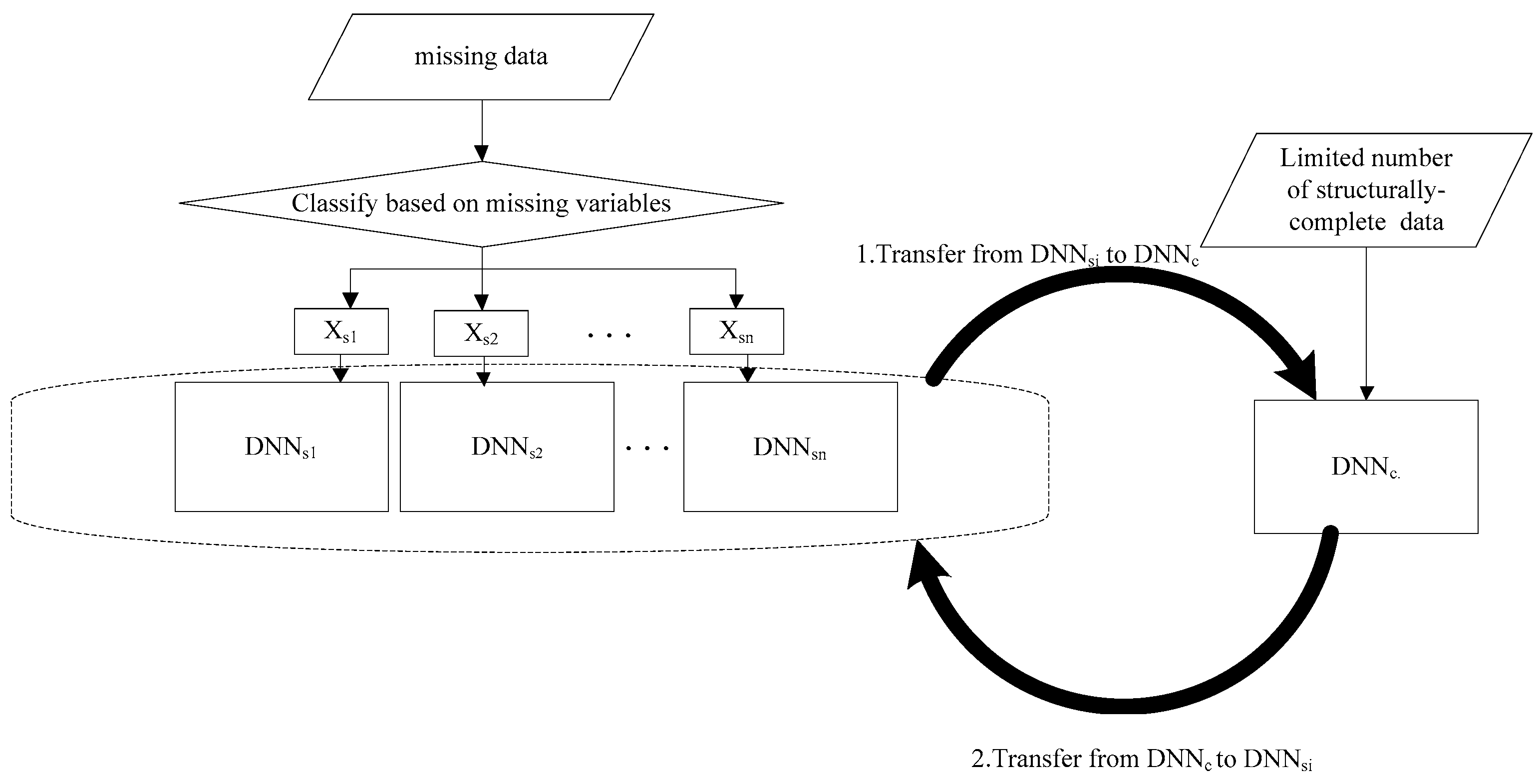
Step 5: Implementing transfer based on multi-rate sampling and building fault diagnosis model of complete data.
Although missing data is incomplete, it still contains fault information. We thus extract fault features from incomplete samples and transfer the extracted features to the structurally complete model to improve the fault diagnosis accuracy of the model. The transfer can cause the structure of
to be modified due to the fact that incomplete and complete samples are different in dimension while the input layer size of the first layer should be the same as the dimensionalities of samples. This transfer process is illustrated in
Figure 3.
for every type of missing data is transferred to
respectively.
represents the model obtained through
migration. Let us take the migration from
to
as an example. At first, the system checks every variable to see if it is missing in
. If the variable is not missing, then the encoding parameter
of the first layer in
can be migrated to the input layer of
. Otherwise the corresponding parameter of the first layer in
is randomly initialized as shown in Equations (18)–(20). It is assumed that structurally-complete data has
P variables while incomplete data has
variables. Without loss of generality, the
variables of incomplete data can be assumed to be the first
variables of structurally-complete data. r represents a random number. The encoding parameters of the remaining layers in
are migrated to
in Equation (21). The decoding parameters
of the first layer in
can be similarly migrated to
as shown in Equations (22)–(24). Last but not least, the decoding parameters of the remaining layers in
are migrated to
as indicated in Equation (25).
Therefore, we build fault diagnosis model of complete data by transfer learning . are also built in the similar way to .
Step 6: Training the models .
Still taking as an example, is trained by structural complete data set and features are obtained by . The model updates parameters by Equations (5) and (6).
Step 7: Optimizing the models .
is applied to train Softmax model as input data and are optimized by backpropagation algorithm respectively.
3.2. Transfer from Fault Diagnosis Model of Structurally-Complete Data to the Model of Missing Data
Although the number of structurally complete samples is small, structurally complete samples contain all the information monitored. Therefore, the structurally complete fault diagnosis model can be migrated to structurally incomplete fault diagnosis models. From all the models , we select one with the highest accuracy which is assumed to be . Then by training and optimizing the model repeatedly, a better model can be obtained and in turn migrated to .
Step 1: Transferring from fault diagnosis model of structurally-complete data to the model of missing data.
Structurally-complete data contains the overall information of the fault despite the fact that the sample size is limited. Therefore, complete samples can also be made full use of to extract fault features which are then transferred to the model of incomplete data for a higher accuracy of fault diagnosis. According to the dimensionalities of complete and incomplete samples, the input layer size of
is more than
. We use the migration from
to
as an example. Firstly, the system checks
for missing any variables. Secondly, the encoding parameters
of the first layer in
can be migrated to the input layer of
as indicated in Equation (26). Under the assumption that structurally-complete data has
P variables while incomplete data has
variables, the
variables of incomplete data can be considered as the first
variables of structurally-complete data without loss of generality. This is shown in Equations (27) and (28). Thirdly, the decoding parameters
of the first layer in
can be migrated to
in Equation (30)–(32). Fourthly, the encoding and decoding parameters of the remaining layers in
can be migrated to
as indicated in Equations (29) and (33).
Step 2: Building fault diagnosis models for each type of missing data.
Let us take type i as an example and build its fault diagnosis model .
Step 3: Training the models .
Taking as an example, is trained by historical missing data set and obtained features is shown in . is used as input data to train Softmax model and the model updates parameters .
Step 4: Optimizing the models .
Using as an example again, is optimized by backpropagation algorithm. In this way, and are trained alternately until a satisfactory accuracy of fault diagnosis is achieved.


