Aggregation of GPS, WLAN, and BLE Localization Measurements for Mobile Devices in Simulated Environments


Abstract
:1. Introduction
2. Proposed Location-Aggregation Method
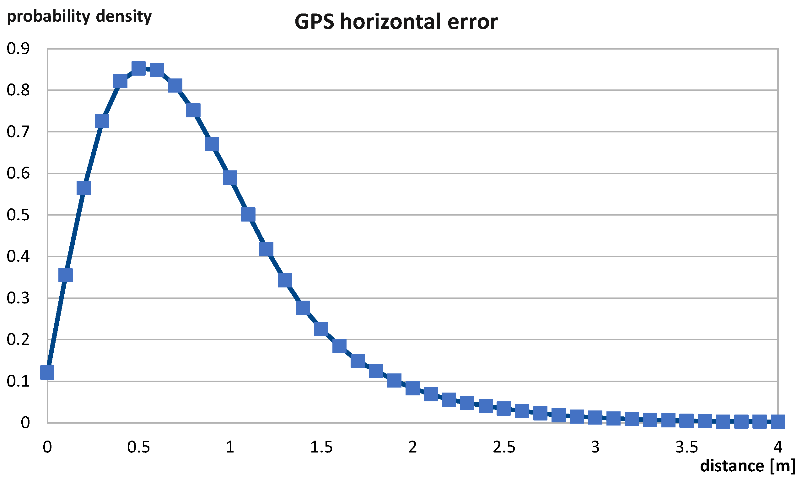
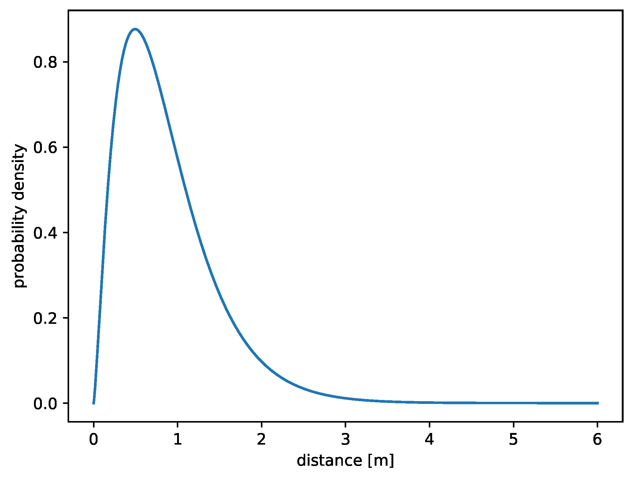
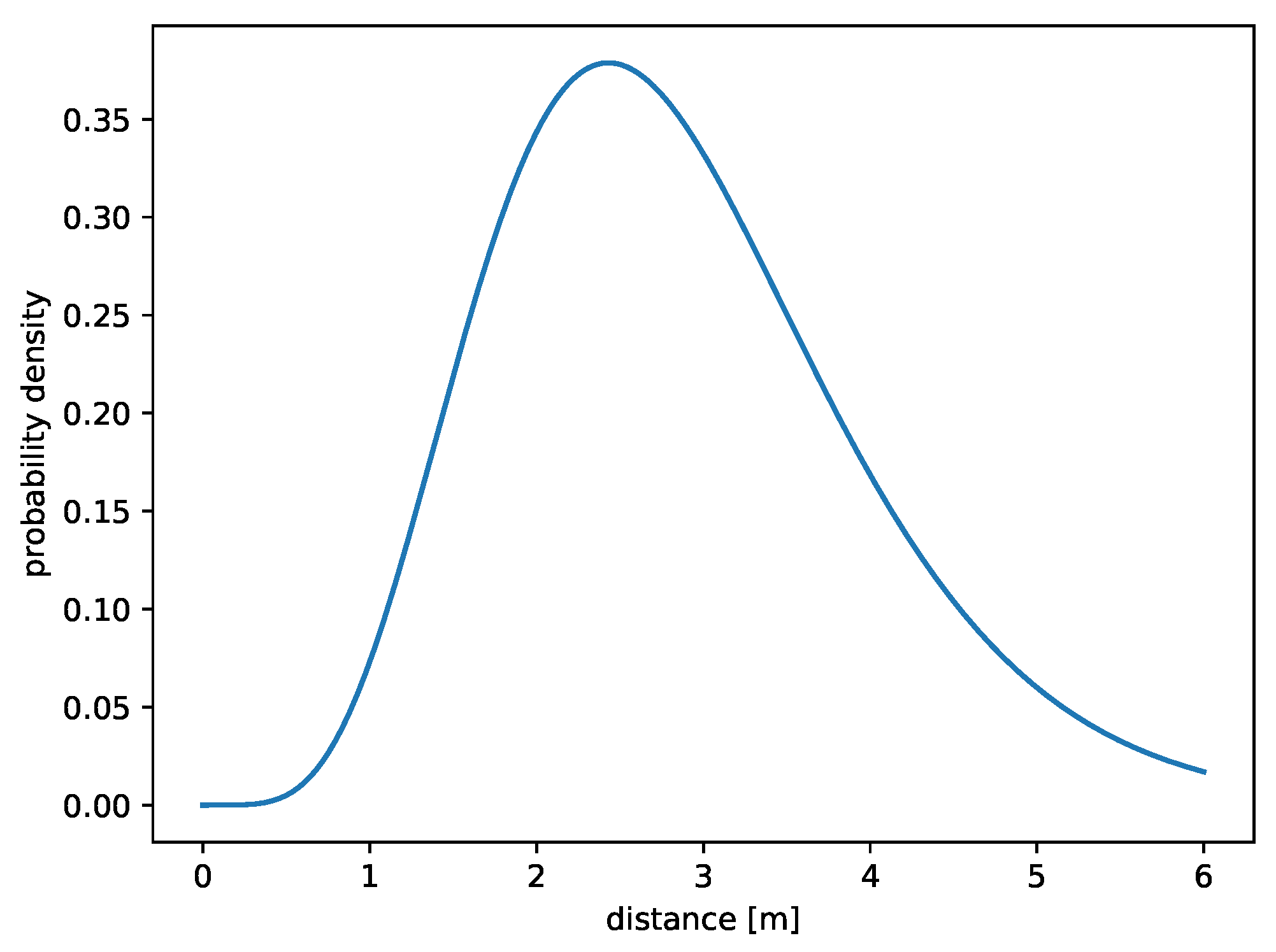
2.1. Error-Distribution Fitting
2.2. GPS
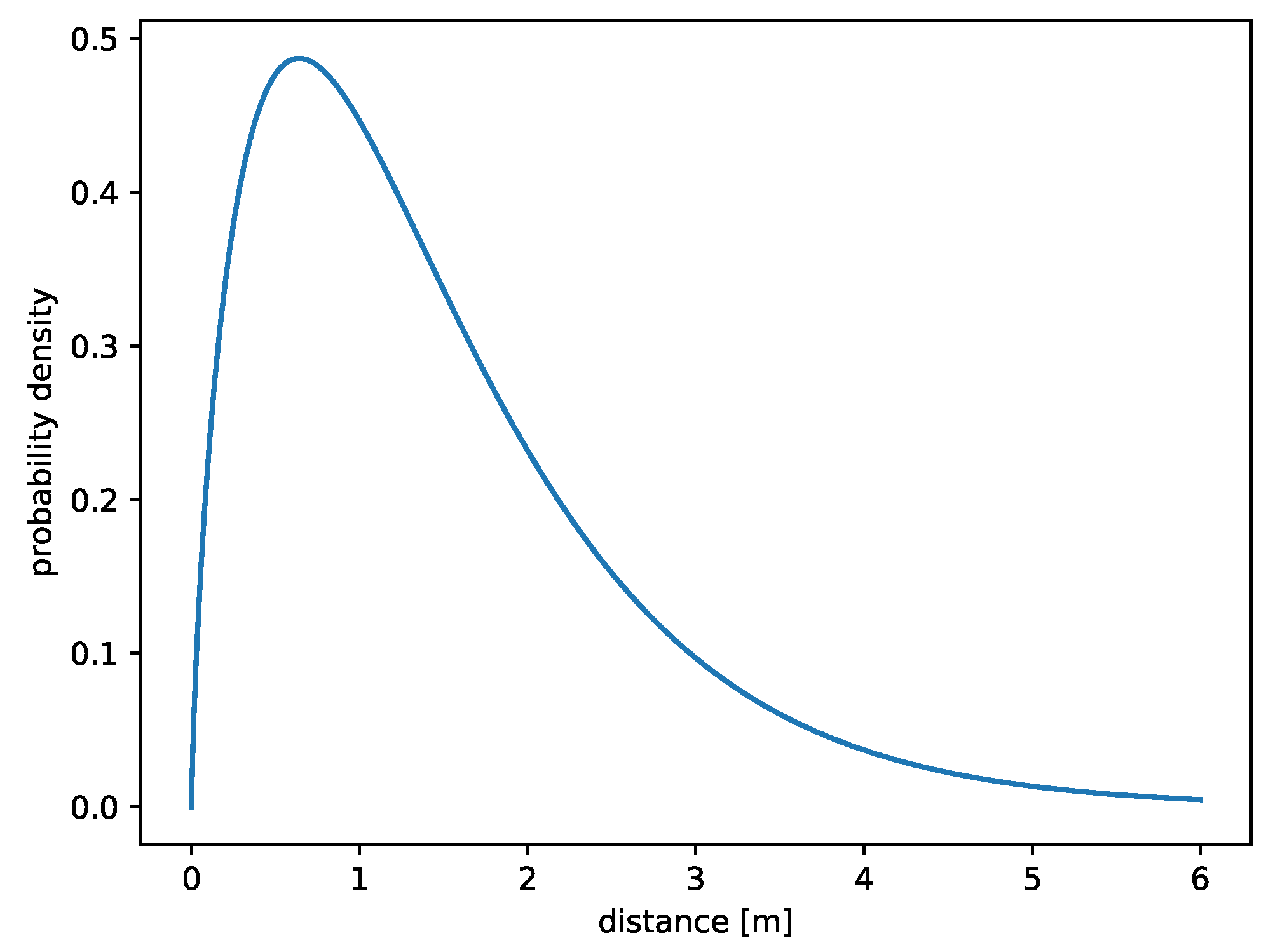
2.3. WLAN
2.4. BLE Beacons
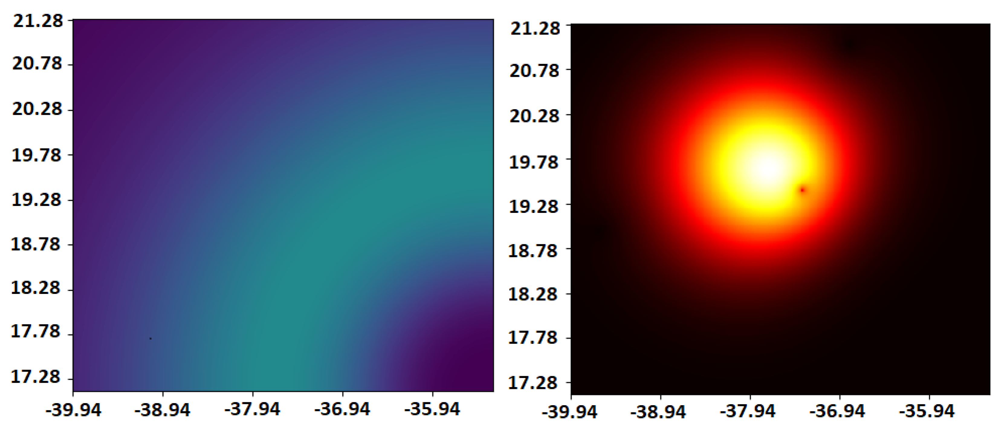
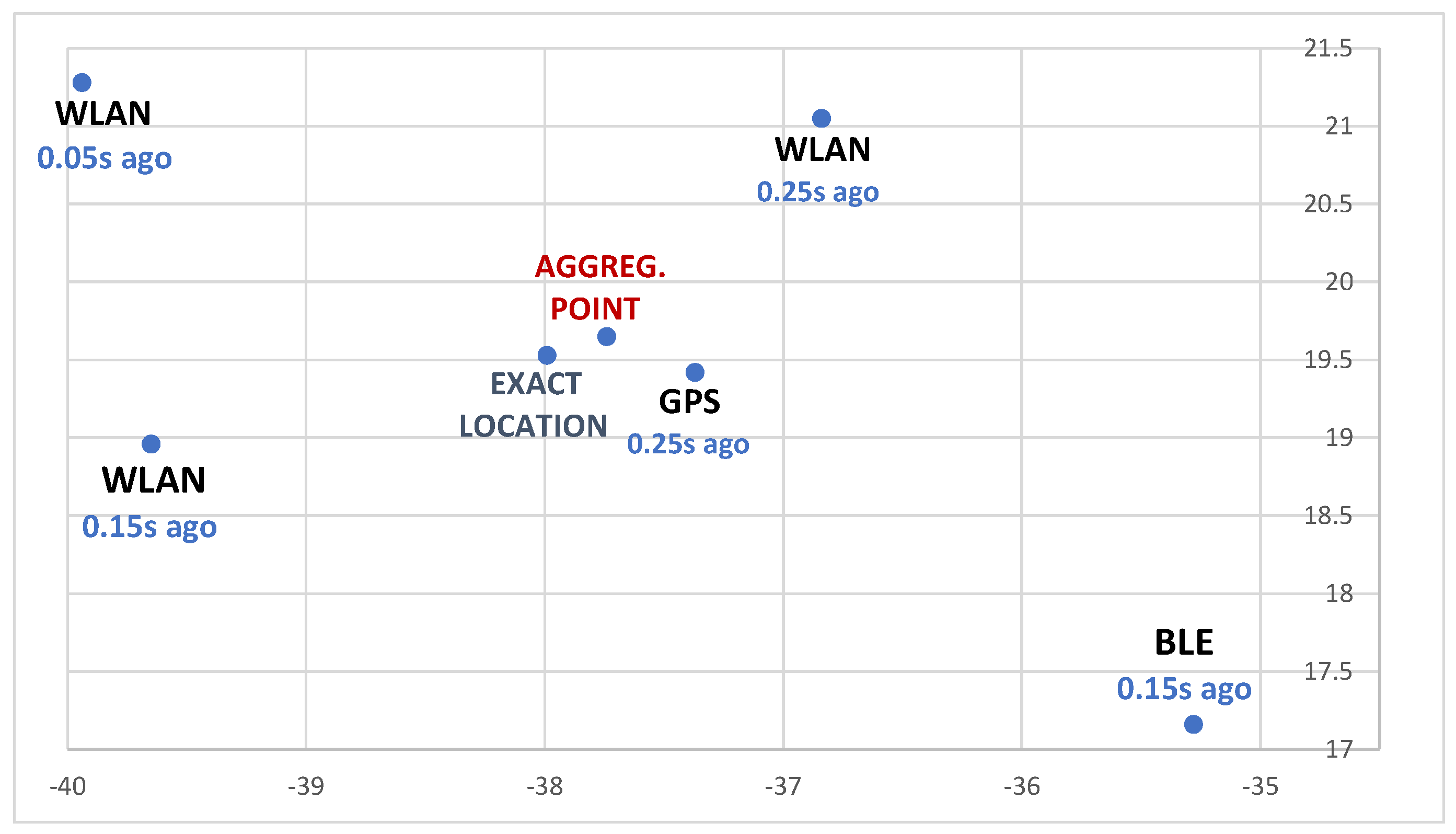
2.5. Location Aggregation
| Algorithm 1 Pseudocode of the localization-aggregation method |
| Input: Points indicated by used methods with timestamps: GPS ; , WLAN , , BLE , , distributions of errors of GPS (), WLAN () and (), present timestamp t Output: Coordinates of the optimum with value of function (Equation (10)) Calculate range of calculations:
|
3. Aggregation-Accuracy Analysis
3.1. Movement Model
3.2. Simulation Model
- a mobile node moves according to the Gauss–Markov mobility model with parameters: , , ;
- position of the mobile node changes every 5 ms;
- there exist three localization systems: GPS, WLAN, and BLE beacons; as mentioned before, and they give information about localization every 1000 ms, 100 ms, and 300 ms, respectively;
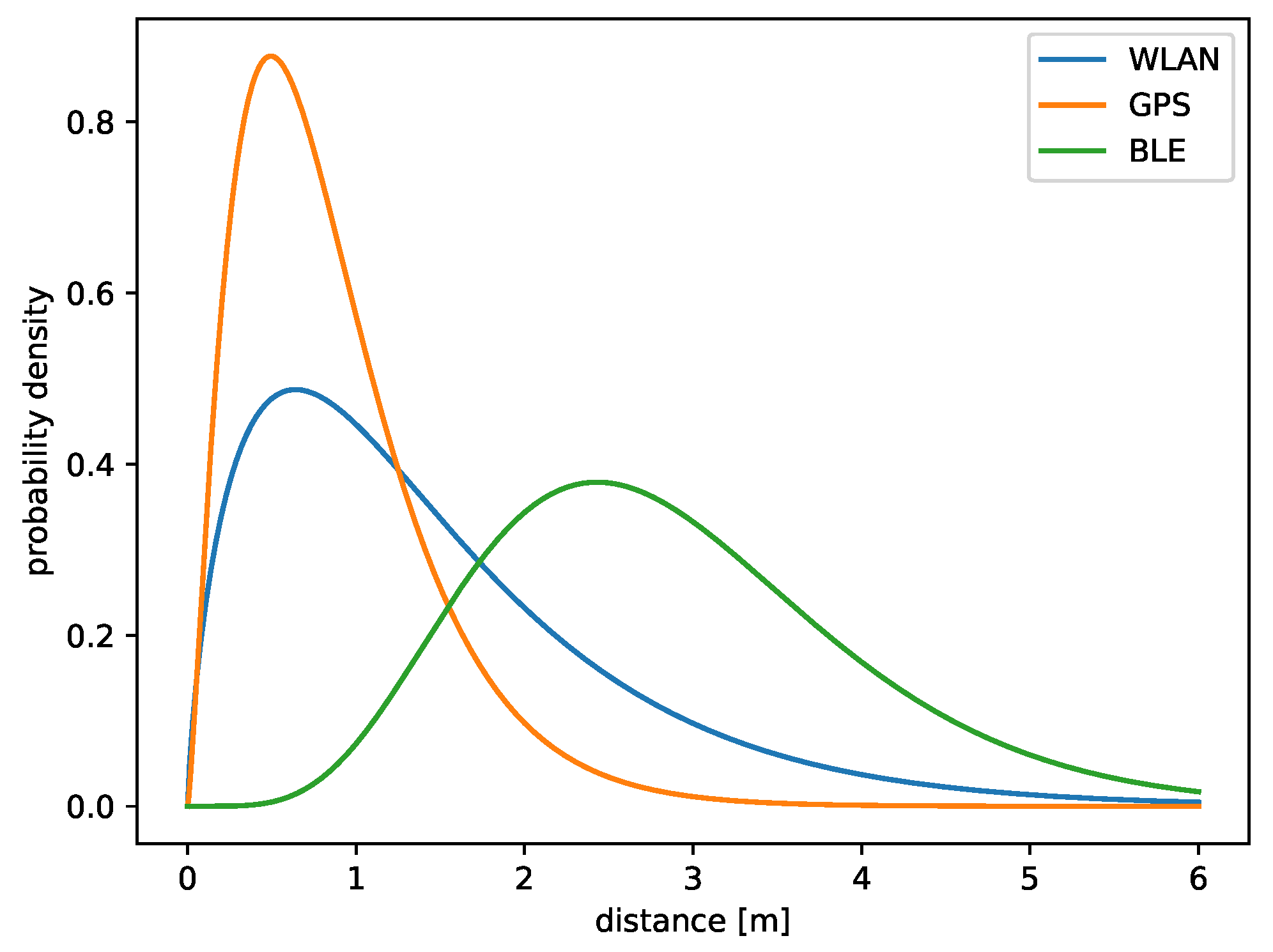
- for successive methods, errors to the actual position are added according to the corresponding distribution error (for instance, GPS errors are pseudorandom values from gamma distribution with shape parameter and scale parameter );
- a position of the mobile node is calculated every 250 ms.
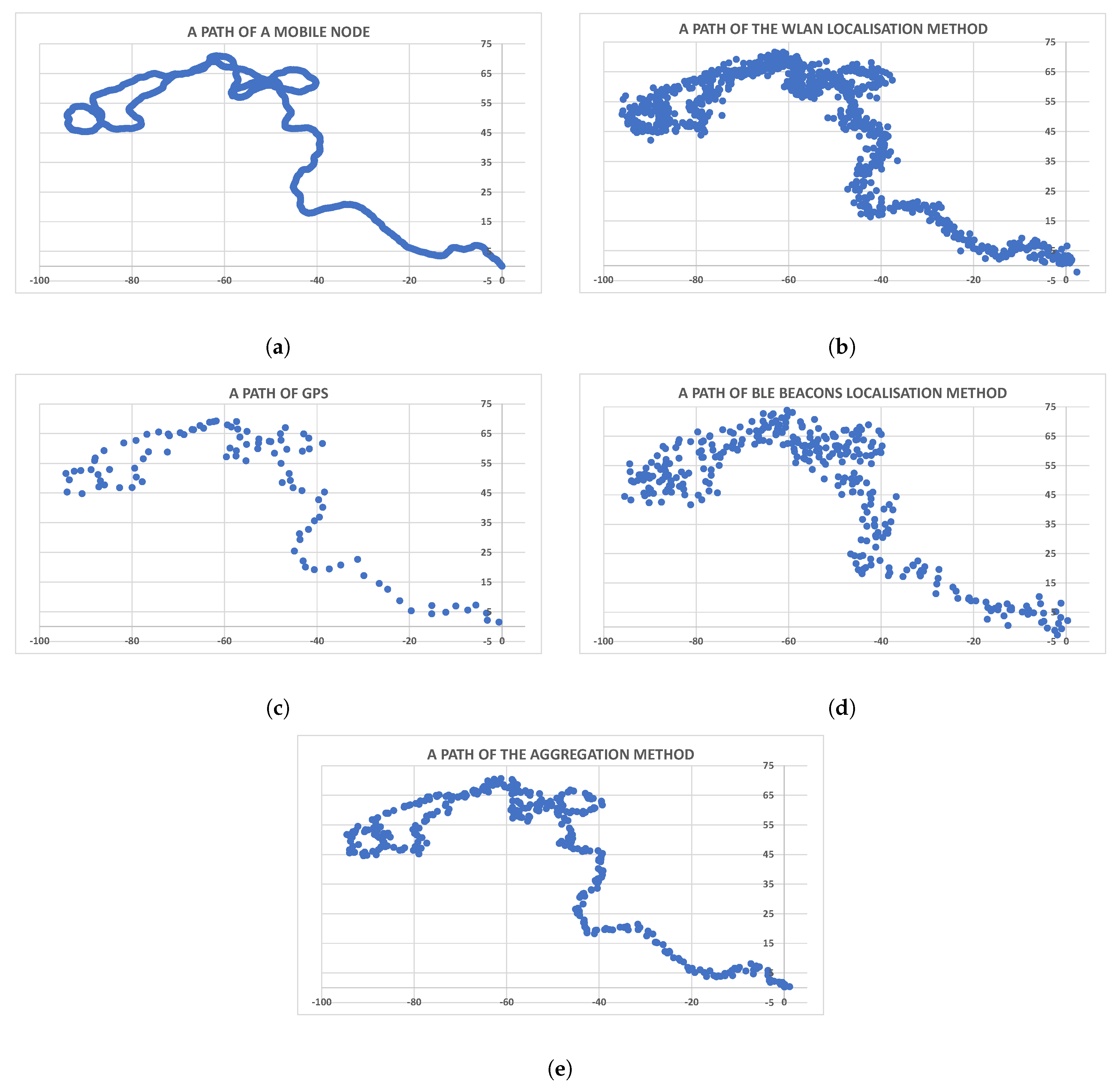
4. Results and Discussion
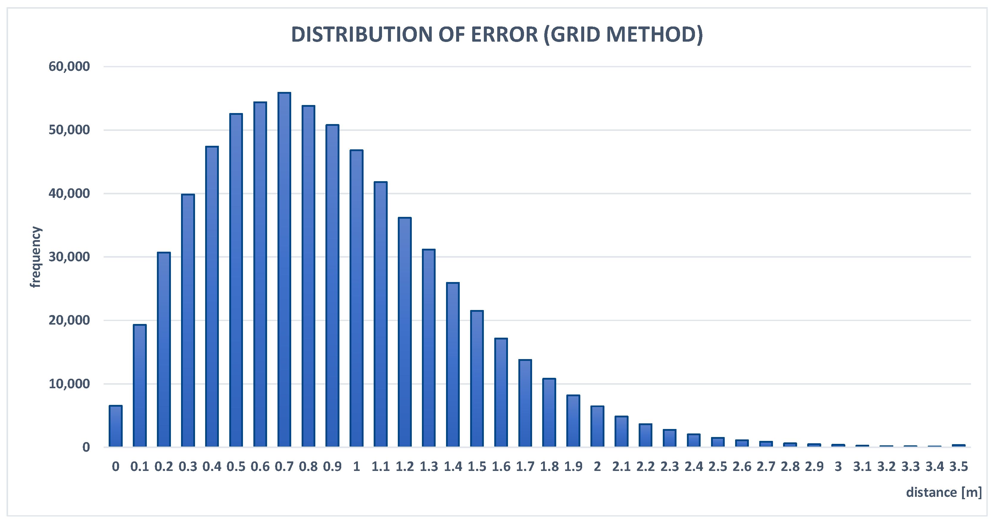
4.1. Aggregation of WLAN, GPS, and BLE Localization
4.2. Aggregation of Only WLAN and GPS
4.3. Adaptation to Different Positioning System Error Characteristics
5. Conclusions and Future Work
Author Contributions
Funding
Conflicts of Interest
References
- Rajalakshmi, K.; Goyal, M. Location-Based Services: Current State of The Art and Future Prospects. In Optical and Wireless Technologies; Springer: Berlin/Heidelberg, Germany, 2018; pp. 625–632. [Google Scholar]
- Cisco Visual Networking Index. Forecast and Methodology, 2016–2021. September 2017. 2018. Available online: https://www.cisco.com/c/en/us/solutions/collateral/service-provider/visualnetworking-index-vni/complete-white-paper-c11-481360.html (accessed on 30 January 2019).
- Xu, G.; Xu, Y. GPS: Theory, Algorithms and Applications; Springer: Berlin/Heidelberg, Germany, 2016. [Google Scholar]
- Kjærgaard, M.B.; Blunck, H.; Godsk, T.; Toftkjær, T.; Christensen, D.L.; Grønbæk, K. Indoor positioning using GPS revisited. In International Conference on Pervasive Computing; Springer: Berlin/Heidelberg, Germany, 2010; pp. 38–56. [Google Scholar]
- Jekabsons, G.; Kairish, V.; Zuravlyov, V. An analysis of Wi-Fi based indoor positioning accuracy. Sci. J. Riga Tech. Univ. Comput. Sci. 2011, 44, 131–137. [Google Scholar] [CrossRef]
- Google Inc. Get the Last Known Location—Android Developers Documentation. Available online: https://developer.android.com/training/location/retrieve-current (accessed on 22 January 2019).
- Apple Inc. Getting the User’s Location—Apple Developer Documentation Archive. Available online: https://developer.apple.com/library/archive/documentation/UserExperience/Conceptual/LocationAwarenessPG/CoreLocation/CoreLocation.html (accessed on 22 January 2019).
- Zou, H.; Jiang, H.; Luo, Y.; Zhu, J.; Lu, X.; Xie, L. Bluedetect: An ibeacon-enabled scheme for accurate and energy-efficient indoor-outdoor detection and seamless location-based service. Sensors 2016, 16, 268. [Google Scholar] [CrossRef] [PubMed]
- Zhang, Y.; Zhang, S.; Li, R.; Guo, D.; Wei, Y.; Sun, Y. WiFi Fingerprint positioning based on clustering in mobile crowdsourcing system. In Proceedings of the 2017 12th International Conference on Computer Science and Education (ICCSE), Houston, TX, USA, 22–25 August 2017; pp. 252–256. [Google Scholar]
- Vavoula, G.; Tseliou, M.A.; Ffoster-Jones, R.; Coleman, S.; Long, P.; Simpson, E. Leicester Castle tells its story beacon-based mobile interpretation for historic buildings. In Proceedings of the 2015 Digital Heritage, Granada, Spain, 28 September–2 October 2015; Volume 1, pp. 411–412. [Google Scholar]
- Kaur, M.J.; Maheshwari, P. Smart tourist for dubai city. In Proceedings of the 2016 2nd International Conference on Next Generation Computing Technologies (NGCT), Dehradun, India, 14–16 October 2016; pp. 30–34. [Google Scholar]
- Baniukevic, A.; Jensen, C.S.; Lu, H. Hybrid indoor positioning with wi-fi and bluetooth: Architecture and performance. In Proceedings of the 2013 IEEE 14th International Conference on Mobile Data Management (MDM), Milan, Italy, 3–6 June 2013; Volume 1, pp. 207–216. [Google Scholar]
- Aparicio, S.; Pérez, J.; Bernardos, A.M.; Casar, J.R. A fusion method based on bluetooth and wlan technologies for indoor location. In Proceedings of the IEEE International Conference on Multisensor Fusion and Integration for Intelligent Systems (MFI 2008), Seoul, Korea, 20–22 August 2008; pp. 487–491. [Google Scholar]
- Liu, J.; Chen, R.; Pei, L.; Guinness, R.; Kuusniemi, H. A hybrid smartphone indoor positioning solution for mobile LBS. Sensors 2012, 12, 17208–17233. [Google Scholar] [CrossRef] [PubMed]
- He, S.; Chan, S.H.G. Wi-Fi fingerprint-based indoor positioning: Recent advances and comparisons. IEEE Commun. Surv. Tutor. 2016, 18, 466–490. [Google Scholar] [CrossRef]
- Deldar, F.; Yaghmaee, M.H. Designing an energy efficient prediction-based algorithm for target tracking in wireless sensor networks. In Proceedings of the 2011 International Conference on Wireless Communications and Signal Processing (WCSP), Nanjing, China, 9–11 November 2011; pp. 1–6. [Google Scholar] [CrossRef]
- Wang, R.; Zhao, F.; Luo, H.; Lu, B.; Lu, T. Fusion of wi-fi and bluetooth for indoor localization. In Proceedings of the 1st International Workshop on Mobile Location-Based Service, Beijing, China, 18 September 2011; ACM: New York, NY, USA, 2011; pp. 63–66. [Google Scholar]
- Cappelle, C.; Pomorski, D.; Yang, Y. GPS/INS data fusion for land vehicle localization. In Proceedings of the Multiconference on Computational Engineering in Systems Applications, Beijing, China, 4–6 October 2006; Volume 1, pp. 21–27. [Google Scholar]
- Senna, J.; Dewberry, B.; Bruemmer, D. Global Positioning System and Ultra Wide Band Universal Positioning Node Consellation Integration. U.S. Patent 15/675,720, 15 February 2018. [Google Scholar]
- Kennedy, J.; Eberhart, R. Particle swarm optimization. In Proceedings of the ICNN’95—International Conference on Neural Networks, Perth, Australia, 27 November–1 December 1995; Volume 4, pp. 1942–1948. [Google Scholar] [CrossRef]
- Particle Swarm Optimization Using C#. Available online: https://visualstudiomagazine.com/Articles/2013/11/01/Particle-Swarm-Optimization.aspx? (accessed on 18 January 2019).
- Clerc, M.; Kennedy, J. The particle swarm-explosion, stability, and convergence in a multidimensional complex space. IEEE Trans. Evol. Comput. 2002, 6, 58–73. [Google Scholar] [CrossRef]
- Global Positioning System (GPS), Standard Positioning Service (SPS), Performance Analysis Report. Available online: http://www.nstb.tc.faa.gov/reports/PAN96_0117.pdf#page=22 (accessed on 18 January 2019).
- Odaka, Y.; In, Y.; Kitazume, M.; Higuchi, M.; Kawasaki, S.; Murakami, H. Error Analysis of the Mobile Phone GPS and Its Application to the Error Reduction. J. Fac. Sci. Tech. Seikei Univ. 2010, 47, 75–81. [Google Scholar]
- Luo, J.; Fu, L. A Smartphone Indoor Localization Algorithm Based on WLAN Location Fingerprinting with Feature Extraction and Clustering. Sensors 2017, 17, 1339. [Google Scholar] [CrossRef]
- Moghtadaiee, V.; Dempster, A.G. Determining the best vector distance measure for use in location fingerprinting. Pervasive Mob. Comput. 2015, 23, 59–79. [Google Scholar] [CrossRef]
- Dahlgren, E.; Mahmood, H. Evaluation of Indoor Positioning Based on Bluetooth Smart Technology. Master’s Thesis, Chalmers University of Technology, Göteborg, Sweden, 2014. [Google Scholar]
- Aarts, E.; Aarts, E.H.; Lenstra, J.K. Local Search in Combinatorial Optimization; Princeton University Press: Princeton, NJ, USA, 2003. [Google Scholar]
- Bai, F.; Helmy, A. A Survey of Mobility Models in Wireless Ad Hoc Networks; University of Southern California: Los Angeles, CA, USA, 2002. [Google Scholar]
- Ariyakhajorn, J.; Wannawilai, P.; Sathitwiriyawong, C. A comparative study of random waypoint and gauss-markov mobility models in the performance evaluation of manet. In Proceedings of the International Symposium on Communications and Information Technologies (ISCIT’06), Bangkok, Thailand, 18–20 October 2006; pp. 894–899. [Google Scholar]


| Distribution | Root-Mean-Squared Error (RMSE) Values | Parameters |
|---|---|---|
| Gamma | 0.01636 | |
| Weibull | 0.01710 | |
| Normal | 0.03513 | |
| Cauchy | 0.05591 | |
| Exponential | 0.11877 |
| Description | Average Error (m) | Relative Error | Standard Deviation |
|---|---|---|---|
| Grid method | 0.94242 | 100.00% | 0.51959 |
| Local Search | 0.94883 | 100.68% | 0.51900 |
| Arithmetic mean | 1.07947 | 114.54% | 0.59607 |
| GPS | 1.49522 | 158.66% | 0.87496 |
| WLAN | 1.50353 | 159.54% | 1.12203 |
| BLE beacons | 2.90712 | 308.47% | 1.18136 |
| Description | Average Error (m) | Relative Error | Standard Deviation |
|---|---|---|---|
| Grid method | 0.95197 | 100.00% | 0.53865 |
| Local Search | 0.96055 | 100.90% | 0.52843 |
| Arithmetic mean | 1.01307 | 106.42% | 0.62801 |
| GPS | 1.49814 | 157.37% | 0.87623 |
| WLAN | 1.50363 | 157.95% | 1.12050 |
© 2019 by the authors. Licensee MDPI, Basel, Switzerland. This article is an open access article distributed under the terms and conditions of the Creative Commons Attribution (CC BY) license (http://creativecommons.org/licenses/by/4.0/).
Share and Cite
Książek, K.; Grochla, K. Aggregation of GPS, WLAN, and BLE Localization Measurements for Mobile Devices in Simulated Environments. Sensors 2019, 19, 1694. https://doi.org/10.3390/s19071694
Książek K, Grochla K. Aggregation of GPS, WLAN, and BLE Localization Measurements for Mobile Devices in Simulated Environments. Sensors. 2019; 19(7):1694. https://doi.org/10.3390/s19071694
Chicago/Turabian StyleKsiążek, Kamil, and Krzysztof Grochla. 2019. "Aggregation of GPS, WLAN, and BLE Localization Measurements for Mobile Devices in Simulated Environments" Sensors 19, no. 7: 1694. https://doi.org/10.3390/s19071694
APA StyleKsiążek, K., & Grochla, K. (2019). Aggregation of GPS, WLAN, and BLE Localization Measurements for Mobile Devices in Simulated Environments. Sensors, 19(7), 1694. https://doi.org/10.3390/s19071694