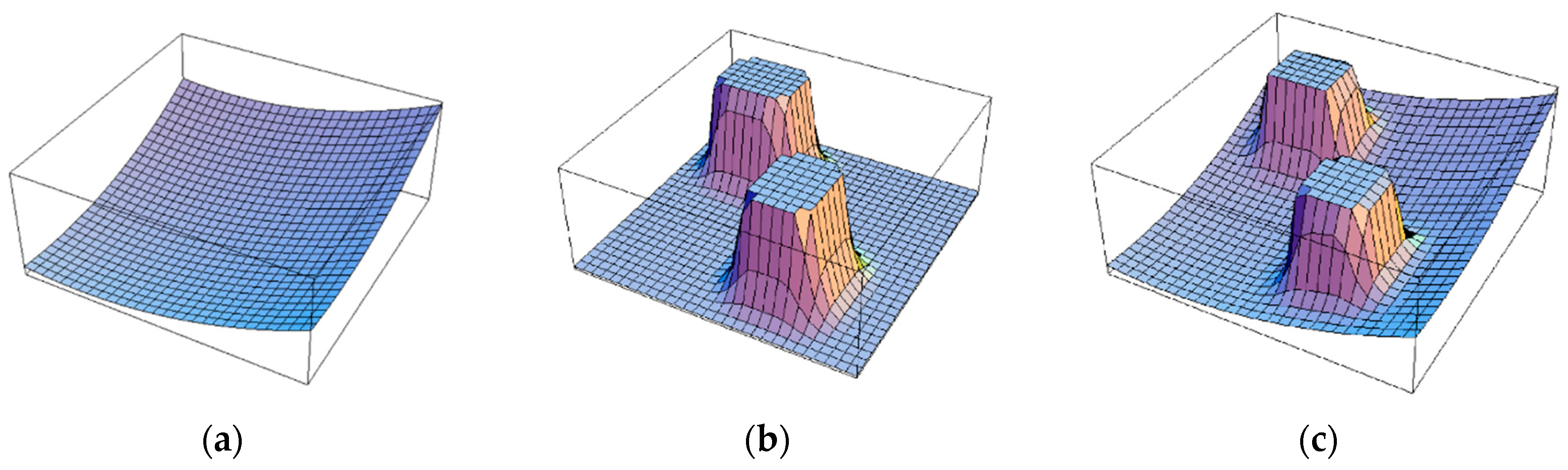
Figure 1.
The potential field method: (a) attractive forces; (b) repulsive forces; and, (c) the sum of attractive forces and repulsive forces for potential filed.
Figure 1.
The potential field method: (a) attractive forces; (b) repulsive forces; and, (c) the sum of attractive forces and repulsive forces for potential filed.
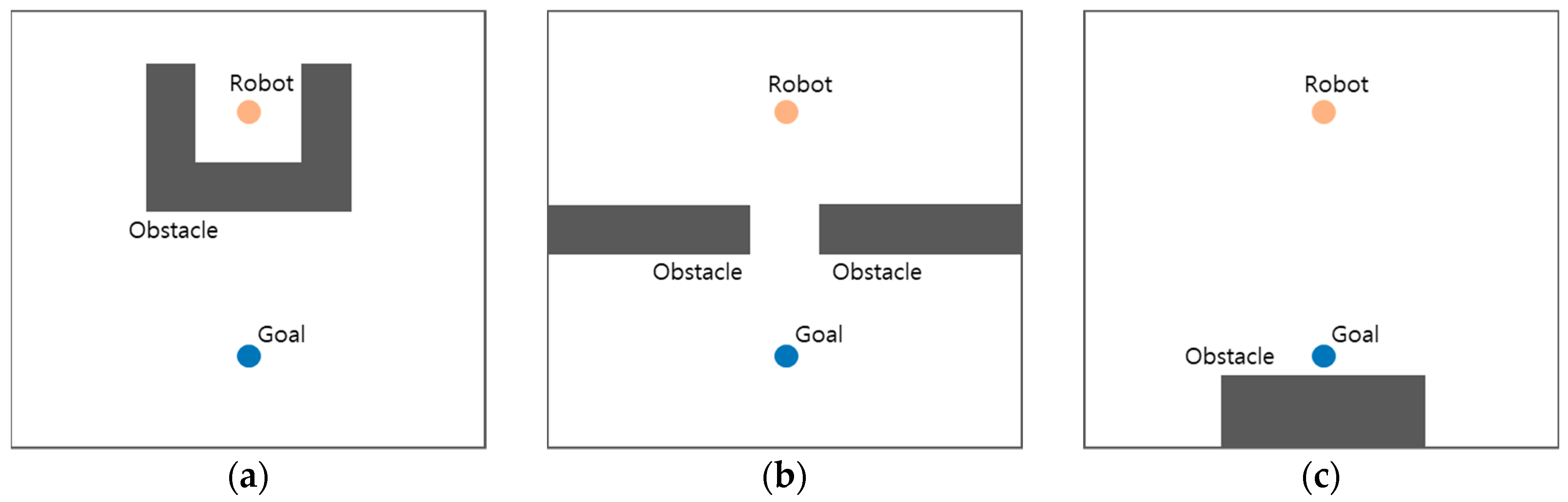
Figure 2.
Representative local minima in a potential field: (a) the robot is surrounded by obstacles and the exit is opposite the goal; (b) narrow distance between obstacles; and, (c) the goal is very close to the obstacles.
Figure 2.
Representative local minima in a potential field: (a) the robot is surrounded by obstacles and the exit is opposite the goal; (b) narrow distance between obstacles; and, (c) the goal is very close to the obstacles.
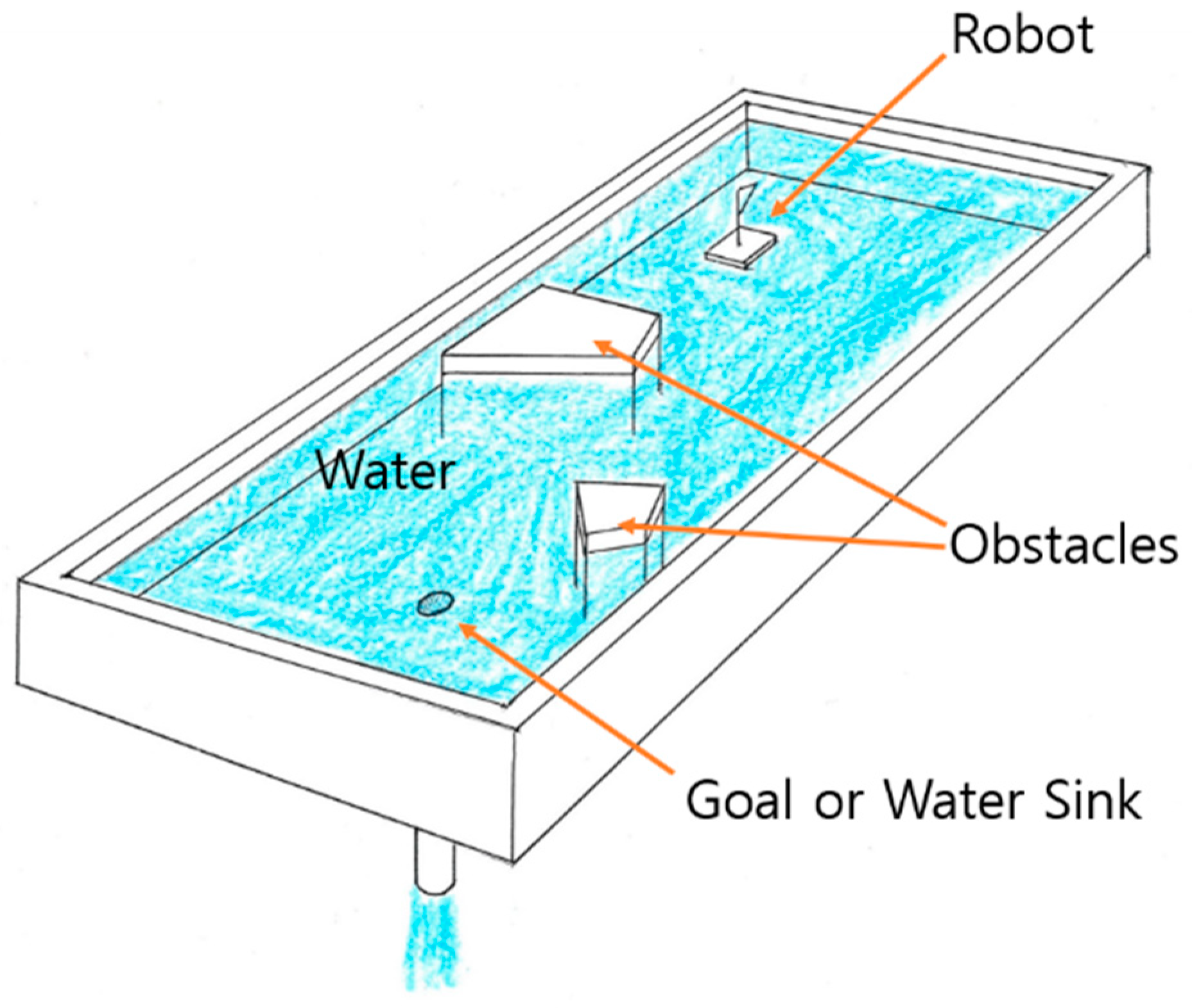
Figure 3.
Water sink model concept.
Figure 3.
Water sink model concept.
Figure 4.
The water sink grid model.
Figure 4.
The water sink grid model.
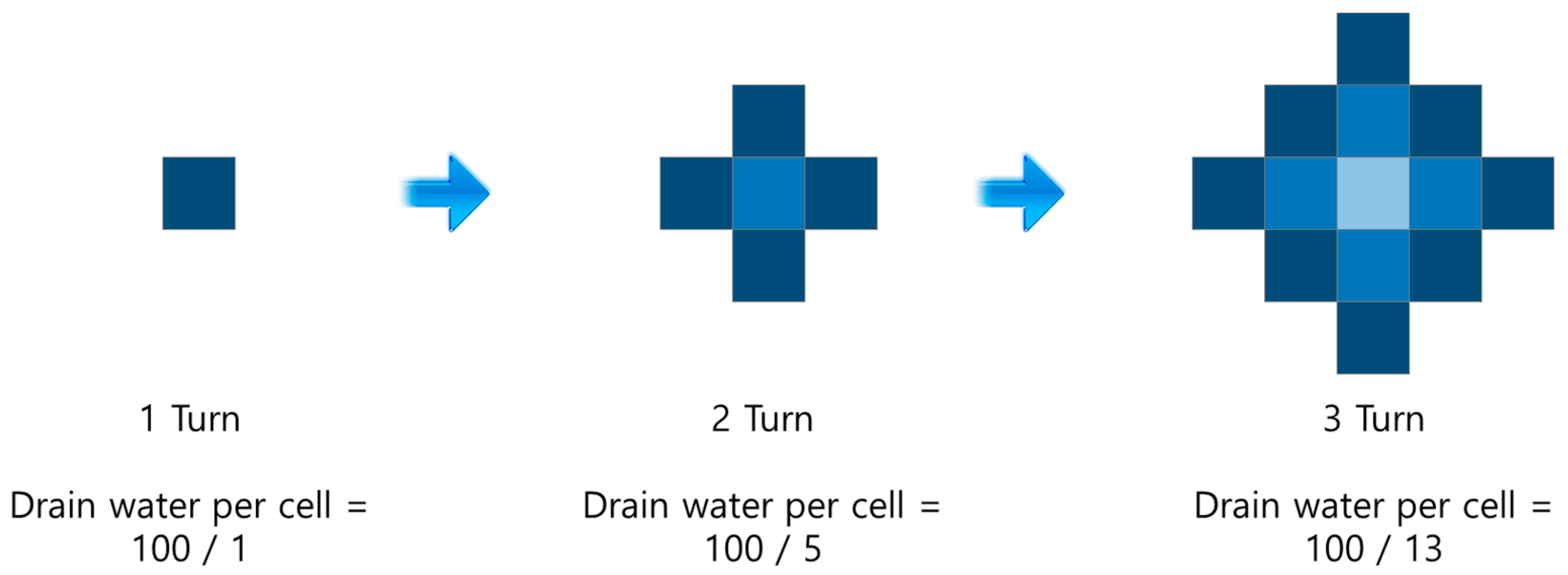
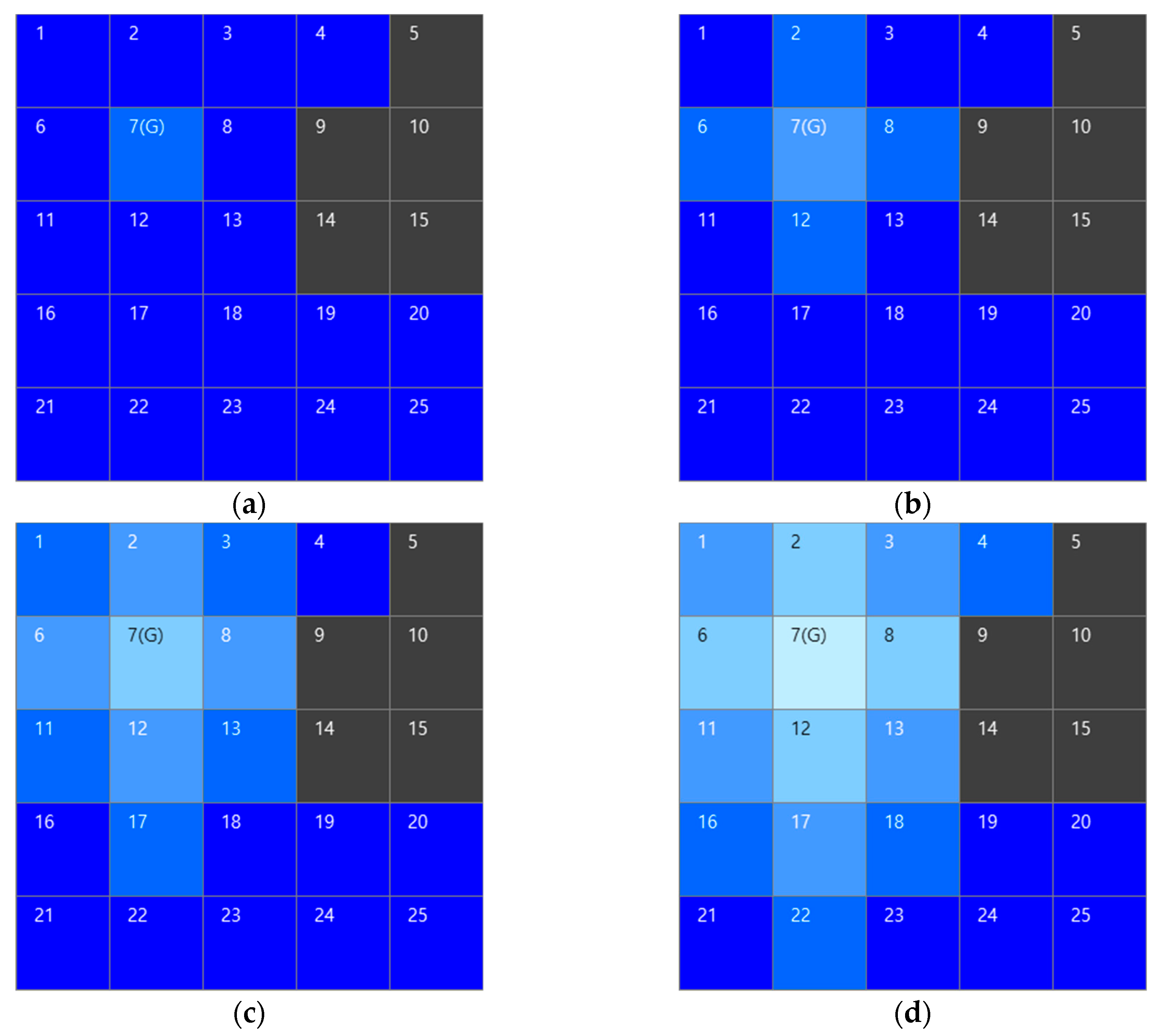
Figure 5.
The sequences of water flow in water sink model. The cell number 7(G) is goal or plug hole and cell number 5, 9, 10, 14, and 15 are obstacles. These examples show the progress of water drainage as: (a) first turn, only plug hole cell is concerned about drainage; (b) second turn, plug hole, and the adjacent cells are involved in drainage; (c) third turn; and, (d) fourth turn, the cells that are involved in the drainage gradually expand and the each cell color becomes gradually brighter.
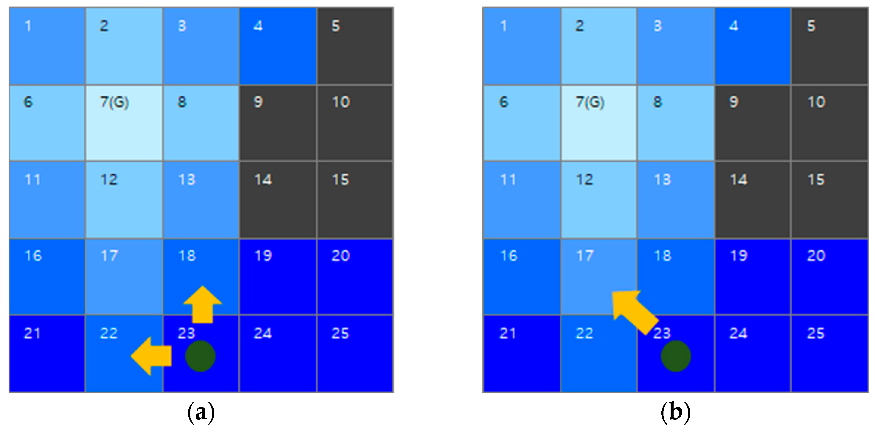
Figure 6.
An example of water sink model-based path generation when using four-connectivity and eight-connectivity: (a) the case of four-connectivity for robot movement; (b) the case of eight-connectivity for robot movement.
Figure 6.
An example of water sink model-based path generation when using four-connectivity and eight-connectivity: (a) the case of four-connectivity for robot movement; (b) the case of eight-connectivity for robot movement.
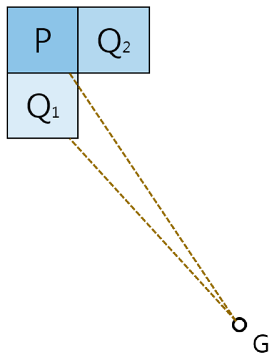
Figure 7.
The case that robot is stopped in another position P, not same with position G.
Figure 7.
The case that robot is stopped in another position P, not same with position G.
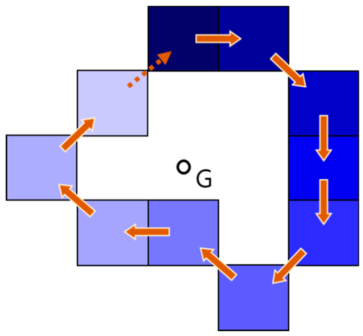
Figure 8.
The case of circular path.
Figure 8.
The case of circular path.
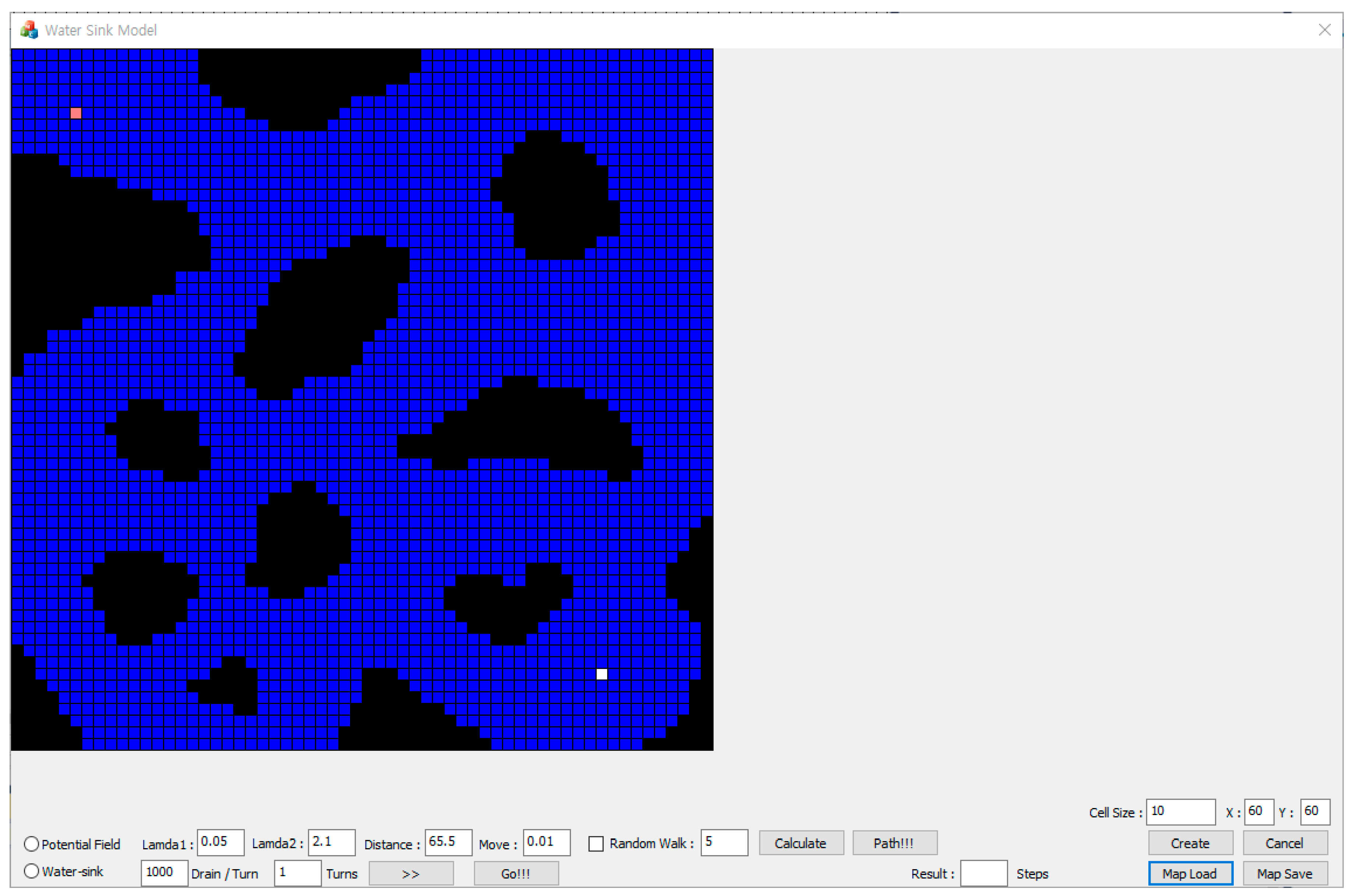
Figure 9.
Water sink model simulator.
Figure 9.
Water sink model simulator.
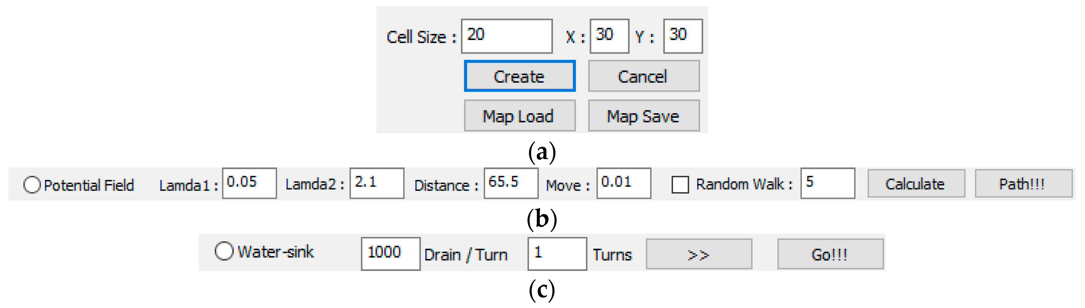
Figure 10.
Parameter adjustment of experimental simulator: (a) map creation part; (b) potential field part; and, (c) water sink model part.
Figure 10.
Parameter adjustment of experimental simulator: (a) map creation part; (b) potential field part; and, (c) water sink model part.
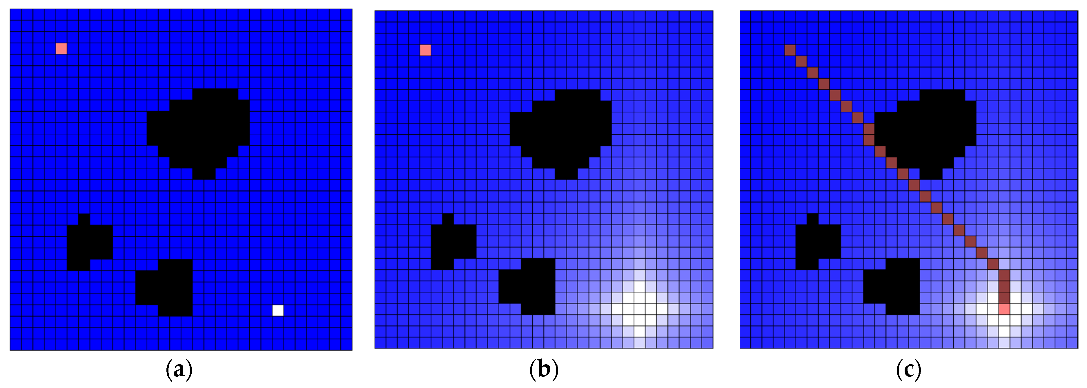
Figure 11.
Water sink model simulator example. Example is 20 (pixels) cell size, 30 × 30 cells and the following is a series of map creation, water drainage, and robot path. The drainage water is 1000 per turn: (a) there are three obstacles, the robot is located at the upper-left corner, and the plughole is located at the lower-right corner; (b) water drainage progressed up to 50 turns; and, (c) final result of robot path.
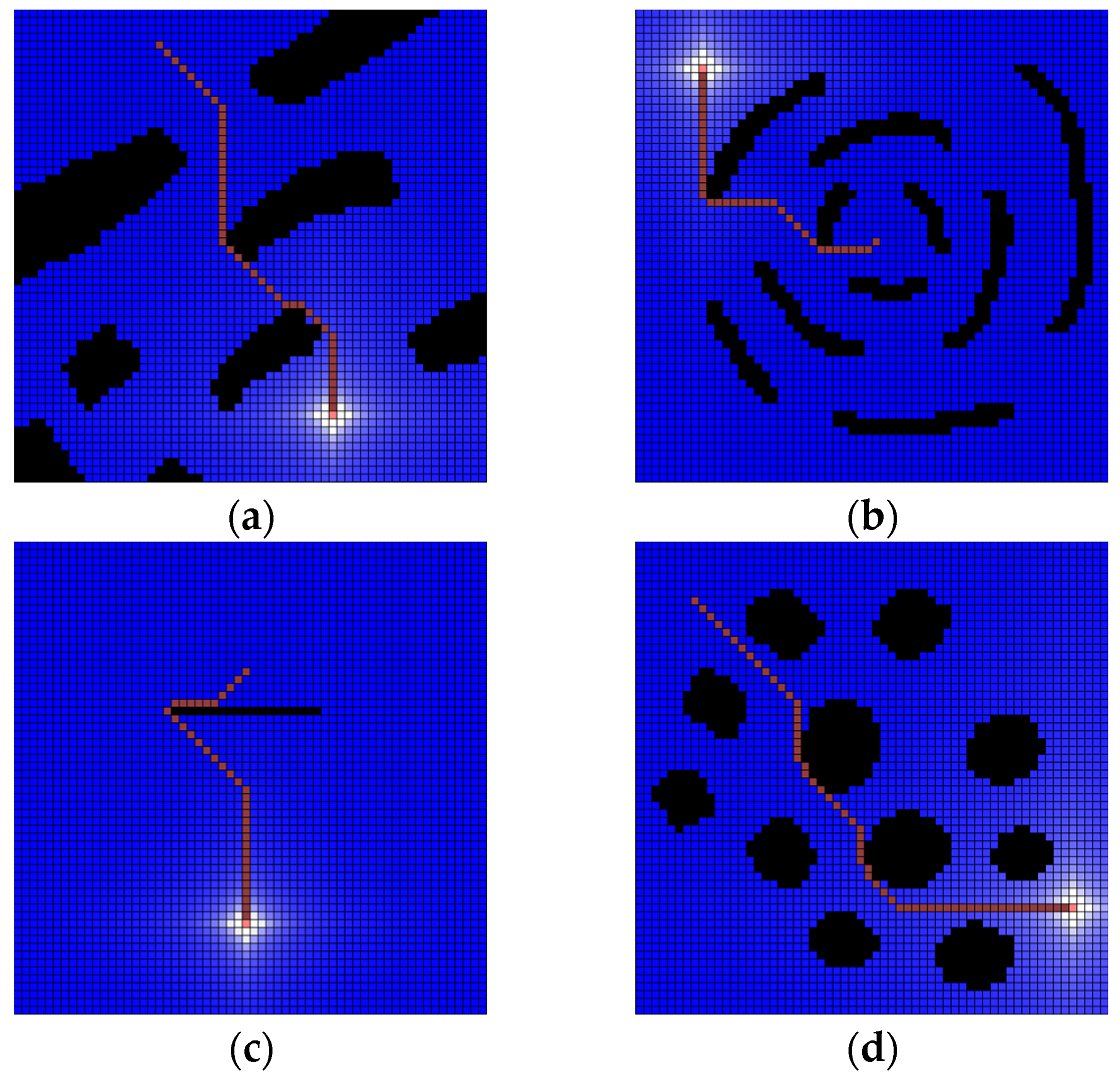
Figure 12.
Several results of water sink model. The cell size is 10 (pixels) and 60 × 60 cells map. The drainage water is 1000 per turn. All experiments show that the robot (pink-colored cell) reached the plughole (white-colored cell) with the shortest path on the grid metric. As a result, the plughole is obscured by the robot: (a) test map-1 for water sink model; (b) test map-2 for water sink model; (c) test map-3 for water sink model; (d) test map-4 for water sink model.
Figure 13.
Several results of potential field method with the same map of water sink model in
Figure 12: (
a) test map-1 for potential field method; (
b) test map-2 for potential field method; (
c) test map-3 for potential field method; (
d) test map-4 for potential field method.
Figure 13.
Several results of potential field method with the same map of water sink model in
Figure 12: (
a) test map-1 for potential field method; (
b) test map-2 for potential field method; (
c) test map-3 for potential field method; (
d) test map-4 for potential field method.
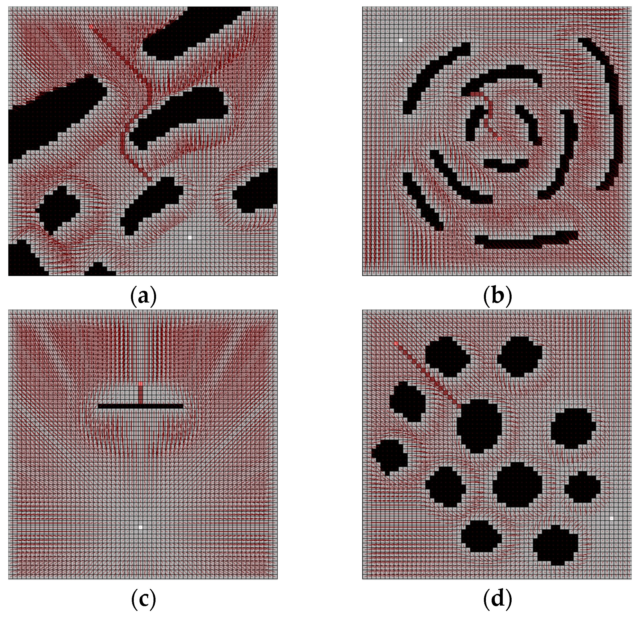
Figure 14.
The results of potential field method with parameter variations.
Figure 14.
The results of potential field method with parameter variations.
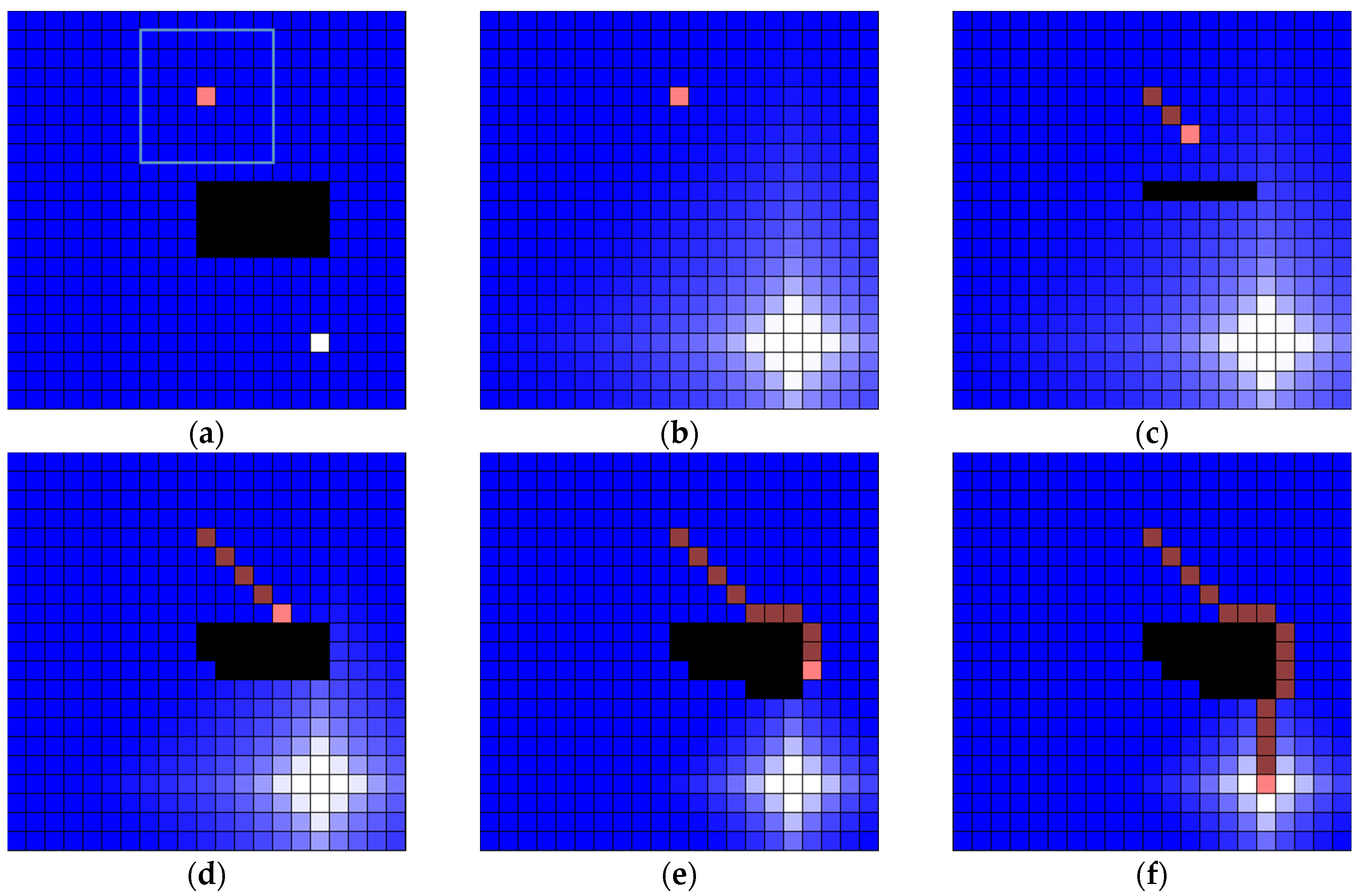
Figure 15.
An example of simulation for dynamic environment. Workspace includes 21 × 21 cells whose size is 20 pixels: (a) there is a 7 × 4 sized obstacle and the sensing area of robot is 7 × 7 cells; (b) the sensor of robot could not detect any obstacle and water drainage is occurred at first; (c) the obstacle could not interfere with the robot path; (d) the robot path is disturbed by an obstacle and water drainage is occurred again; (e) the robot path is disturbed by obstacle again and water drainage is occurred again; and, (f) the final result of water sink model.
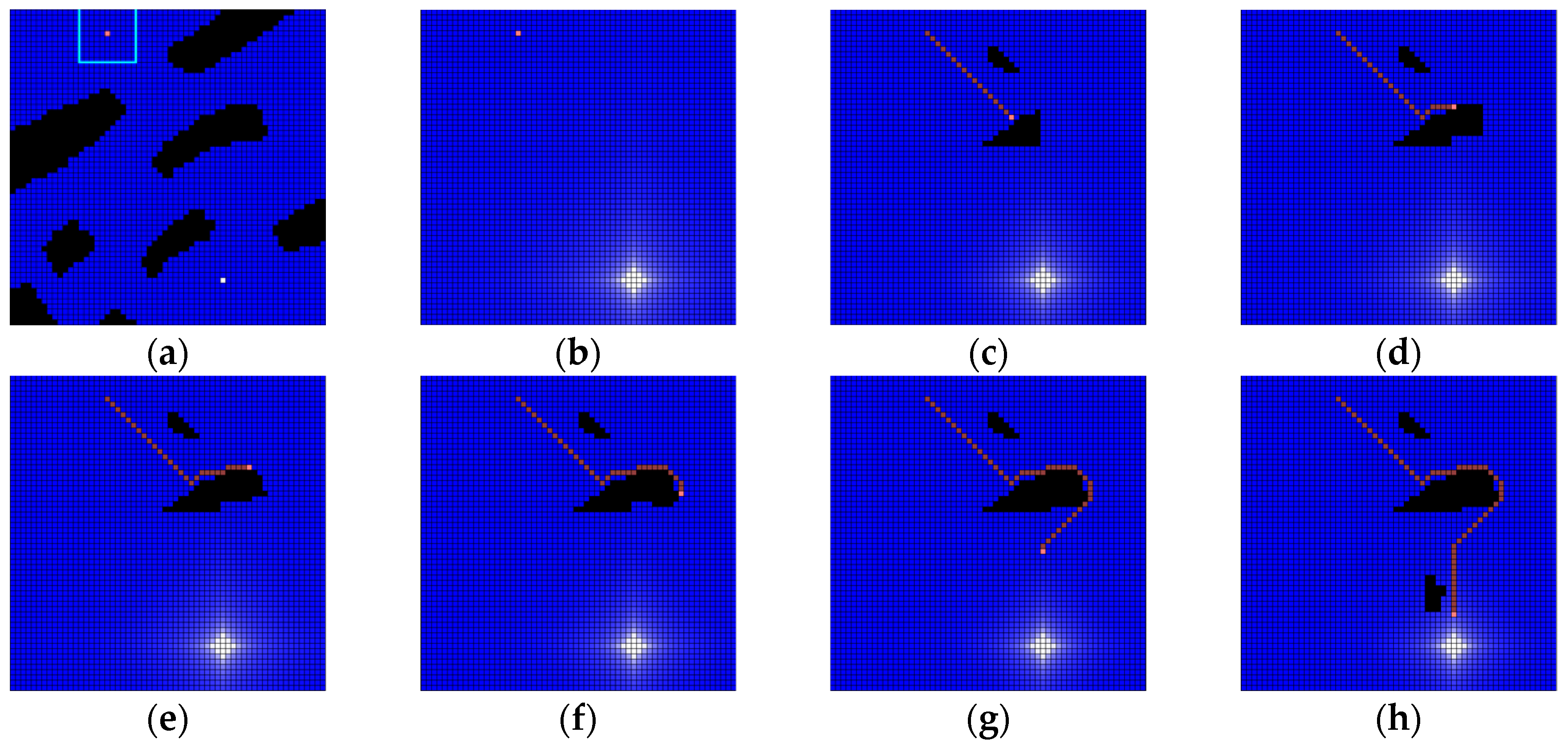
Figure 16.
Another example of simulation for dynamic environment. Workspace includes 60 × 60 cells whose size is 10 pixels: (a) there are some obstacles and the sensing area of robot is 11 × 11 cells; (b) the sensor of robot could not detect any obstacle and water drainage is occurred at first; (c) the robot encounters some obstacles at first; (d–f) the robot path is disturbed by an obstacle and water drainage is occurred again; (g) the robot escapes the obstacle area; and, (h) some obstacles are found, but there is no interference with the robot path. Finally, the robot could reach the plughole.
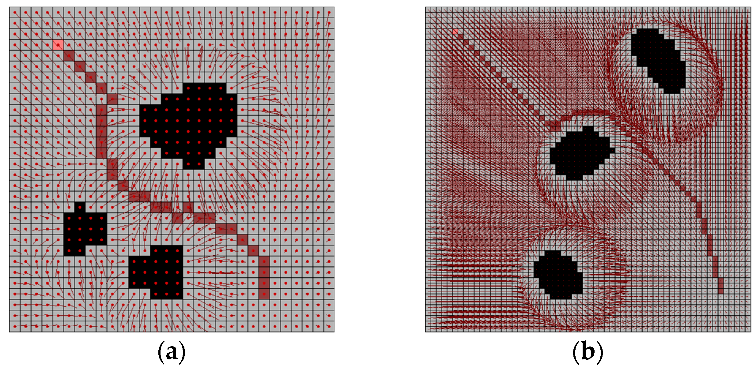
Figure 17.
The potential field maps for comparison with water sink model: (a) map-1: 30 × 30 size map; and, (b) map-2: 60 × 60 size map.
Figure 17.
The potential field maps for comparison with water sink model: (a) map-1: 30 × 30 size map; and, (b) map-2: 60 × 60 size map.
Figure 18.
The results of water sink model. The path length is (
a) map-1: 23, the same as
Figure 10c; and, (
b) map-2: 57.
Figure 18.
The results of water sink model. The path length is (
a) map-1: 23, the same as
Figure 10c; and, (
b) map-2: 57.
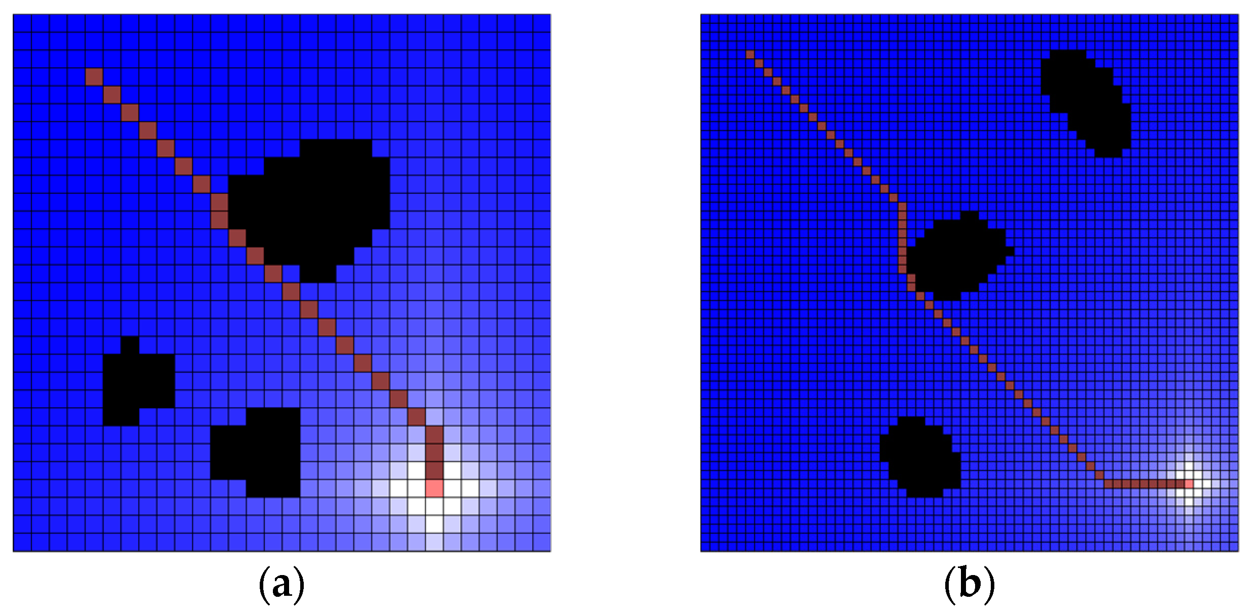
Figure 19.
The results of water sink model. The path length is: (a) map-1: 23; and, (b) map-2: 57.
Figure 19.
The results of water sink model. The path length is: (a) map-1: 23; and, (b) map-2: 57.
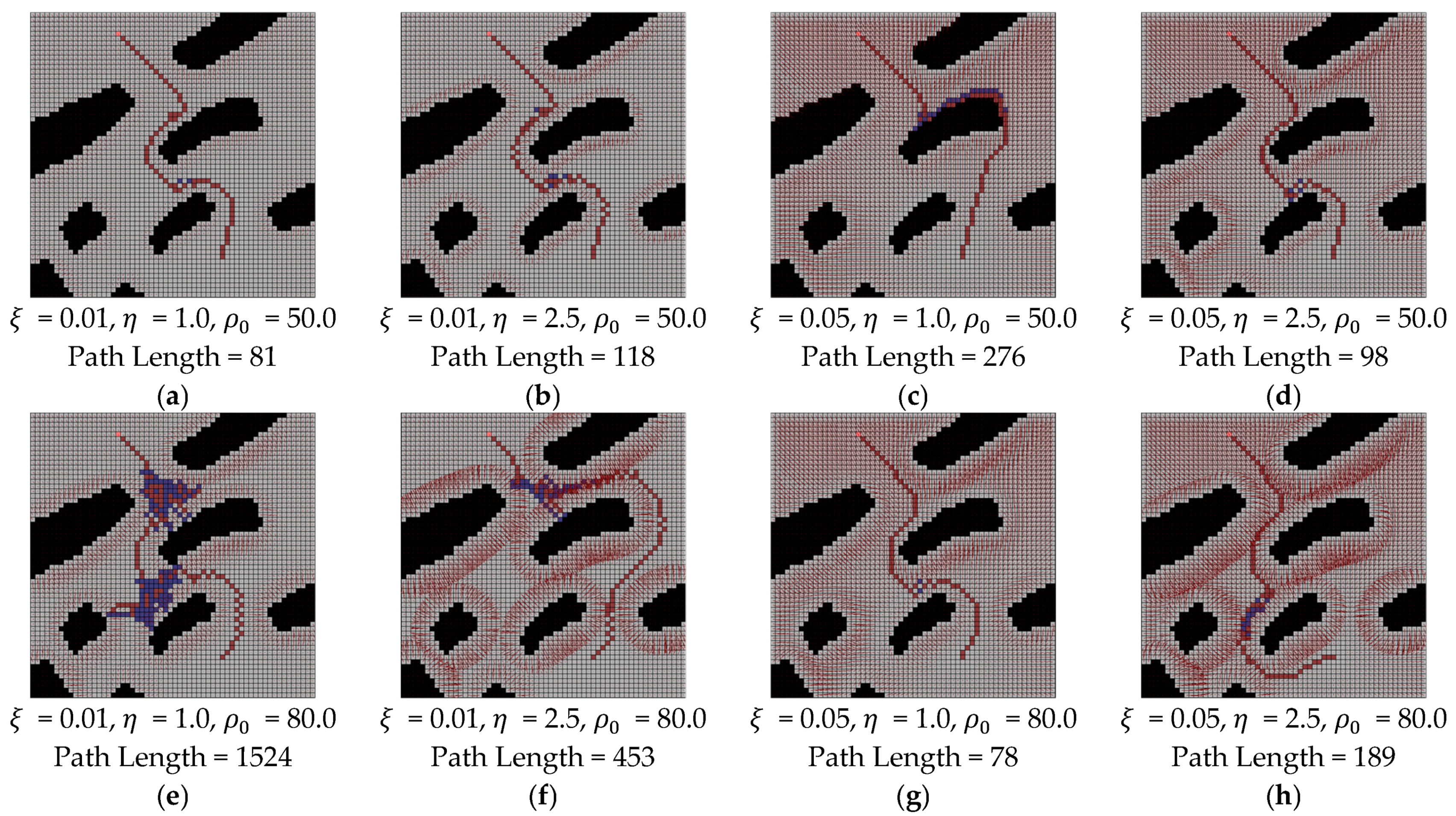
Figure 20.
The results of potential field method using random walk with parameter variations.
Figure 20.
The results of potential field method using random walk with parameter variations.
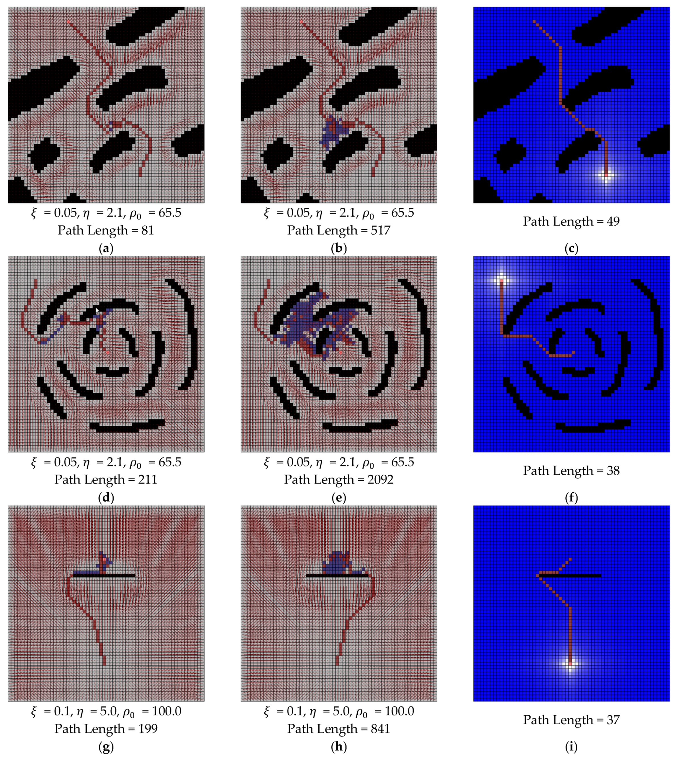
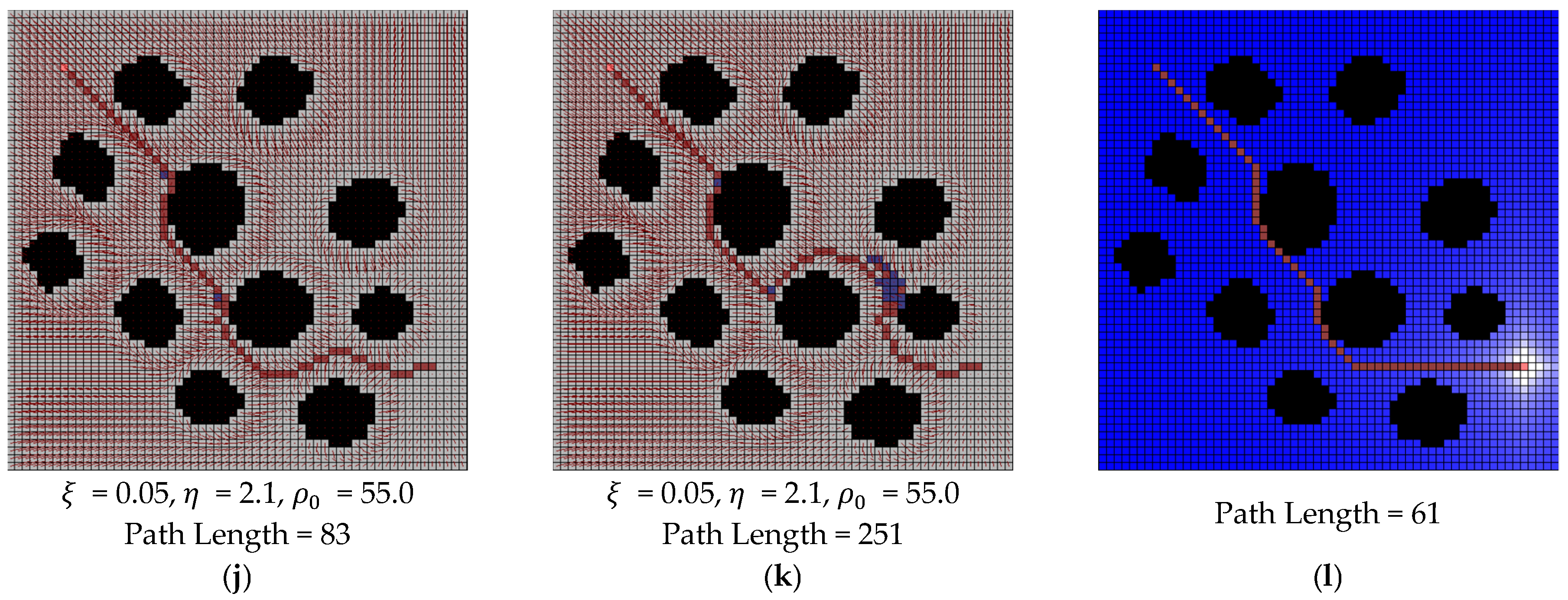
Figure 21.
The results of comparison between water sink model and potential field with random walk: (a,b,d,e) parameters are , and ; (g,h) parameters are , and ; (j,k) parameters are , and ; (c,f,i,l) are the results of water sink model.
Figure 21.
The results of comparison between water sink model and potential field with random walk: (a,b,d,e) parameters are , and ; (g,h) parameters are , and ; (j,k) parameters are , and ; (c,f,i,l) are the results of water sink model.
Table 1.
The characteristics of parameters for potential field method.
Table 1.
The characteristics of parameters for potential field method.
| Parameters | | | |
|---|
| small value | The robot could not move from the beginning | The robot could move around obstacles | Fail to reflect overall obstacle situation |
| large value | The robot could stop when encountering an obstacle | The robot could move to opposite to the goal | The robot could be affected by obstacles in distant |
Table 2.
Parameter set for map-1 and map-2.
Table 2.
Parameter set for map-1 and map-2.
| Map | | | |
|---|
| map-1 | 0.05, 0.1 | 2, 5 | 50, 100, 150 |
| map-2 | 0.05, 0.1 | 2, 3 | 50, 70, 90 |
Table 3.
Path length on map-1 for potential field method.
Table 3.
Path length on map-1 for potential field method.
| | | Result/Path Length |
|---|
| 0.05 | 2 | 50 | NR 1 |
| 0.05 | 2 | 100 | 23 |
| 0.05 | 2 | 150 | 26 |
| 0.05 | 5 | 50 | 23 |
| 0.05 | 5 | 100 | 25 |
| 0.05 | 5 | 150 | 29 |
| 0.1 | 2 | 50 | NR |
| 0.1 | 2 | 100 | NR |
| 0.1 | 2 | 150 | 23 |
| 0.1 | 5 | 50 | NR |
| 0.1 | 5 | 100 | 23 |
| 0.1 | 5 | 150 | 27 |
Table 4.
Path length on map-2 for potential field method.
Table 4.
Path length on map-2 for potential field method.
| | | Result/Path Length |
|---|
| 0.05 | 2 | 50 | NR 1 |
| 0.05 | 2 | 70 | NR |
| 0.05 | 2 | 90 | NR |
| 0.05 | 3 | 50 | 59 |
| 0.05 | 3 | 70 | NR |
| 0.05 | 3 | 90 | NR |
| 0.1 | 2 | 50 | NR |
| 0.1 | 2 | 70 | NR |
| 0.1 | 2 | 90 | 60 |
| 0.1 | 3 | 50 | NR |
| 0.1 | 3 | 70 | 59 |
| 0.1 | 3 | 90 | 63 |
Table 5.
Comparison of water sink model with potential field method. Averaged path length of potential field, if successful, deterministic path length of water sink model and path length ratio. The unit is cell.
Table 5.
Comparison of water sink model with potential field method. Averaged path length of potential field, if successful, deterministic path length of water sink model and path length ratio. The unit is cell.
| Map | Average Path Length of Potential Field (PF) | Path Length of Water Sink Model (WSM) | Path Length Ratio (WSM/PF) |
|---|
| map-1 | 24.875 | 23 | 0.9246 |
| map-2 | 60.25 | 57 | 0.9461 |


