A Cluster Based Localization Scheme with Partition Handling for Mobile Underwater Acoustic Sensor Networks

Abstract
:1. Introduction
- The relative position of node X with respect to node Y.
- The absolute position of node Y.
- A clustering based mechanism to localize partitioned nodes. Only clusterheads send localization requests on behalf of their cluster. This results in reduction in contention, communication overheads, and energy consumption. Further, this yields a high localization ratio.
- A retransmission control mechanism used by nodes to determine whether, after being localized, they need to retransmit a beacon. This mechanism reduces communication overheads by restricting unnecessary transmission.
- In contrast to other mechanisms, we allow only the GPS node to respond to localization requests. This results in a sharp decrease in responses to localization requests and gives better localization accuracy by avoiding error accumulation.
2. Related Work
3. Methodology
3.1. Definitions
3.2. The Localization Process
- (1)
- Transmission of localization requests with doubled transmission range (In this work we use Evo Logic’s S2CR 48/47 acoustic modem in which transmission range is doubled every next available level of transmission power. Moreover the formulation in Section 4.1 can also be used to calculate the transmission power required to achieve a certain communication range.): At the start of every iteration, all unlocalized nodes or their representative nodes send localization requests with doubled transmission range. If a beacon is not received in response to a localization request, the localization request is sent in the next iteration with doubled transmission range.
- (2)
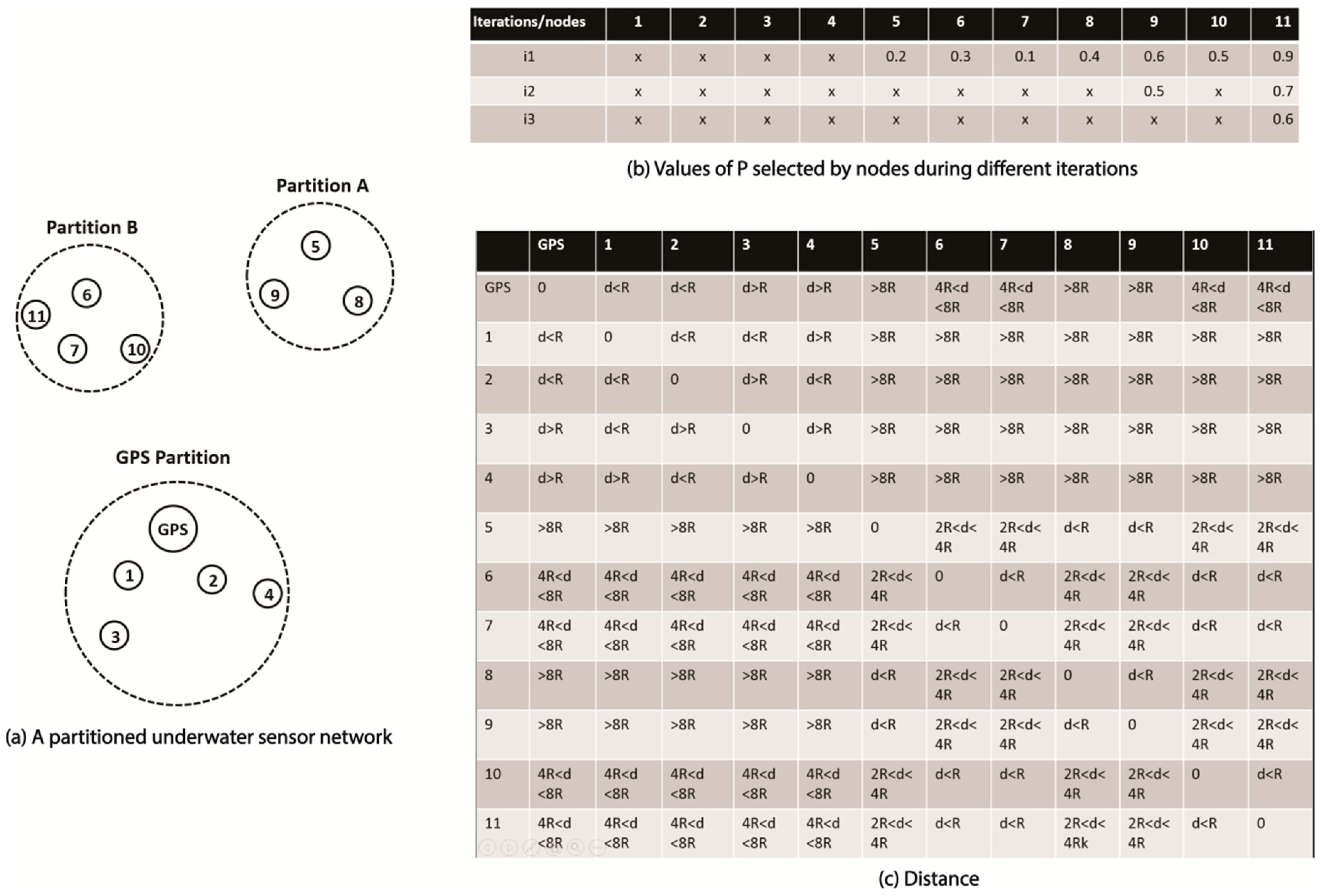
- The selection of cluster heads for the next iteration: Clusterheads (CH) are selected during each iteration based on random values p contained in every localization request. A CH selected during a particular iteration sends localization requests in the next iteration.
- (3)
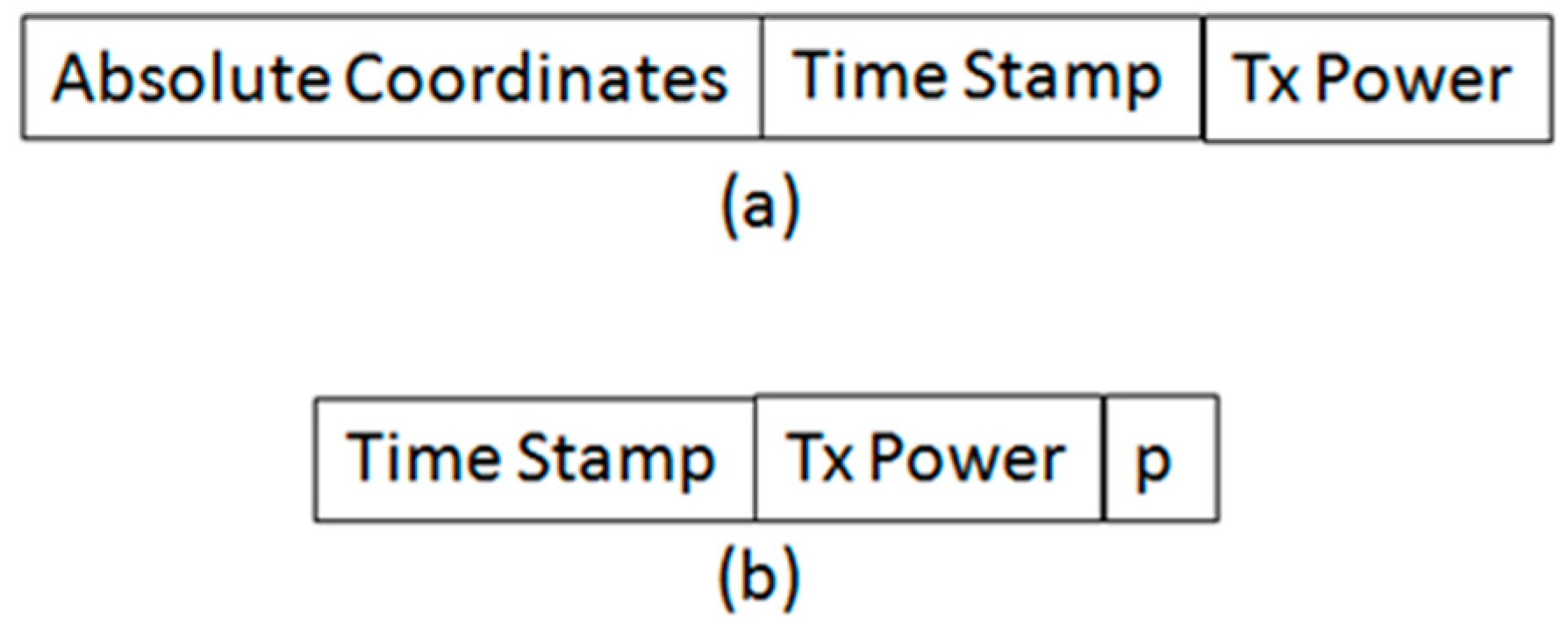
- Reception of localization beacon in response to localization request, and calculation of GPS coordinates using the beacon.
- (4)
- Every freshly localized node runs a “retransmission control” mechanism to decide on the retransmission of an updated beacon.
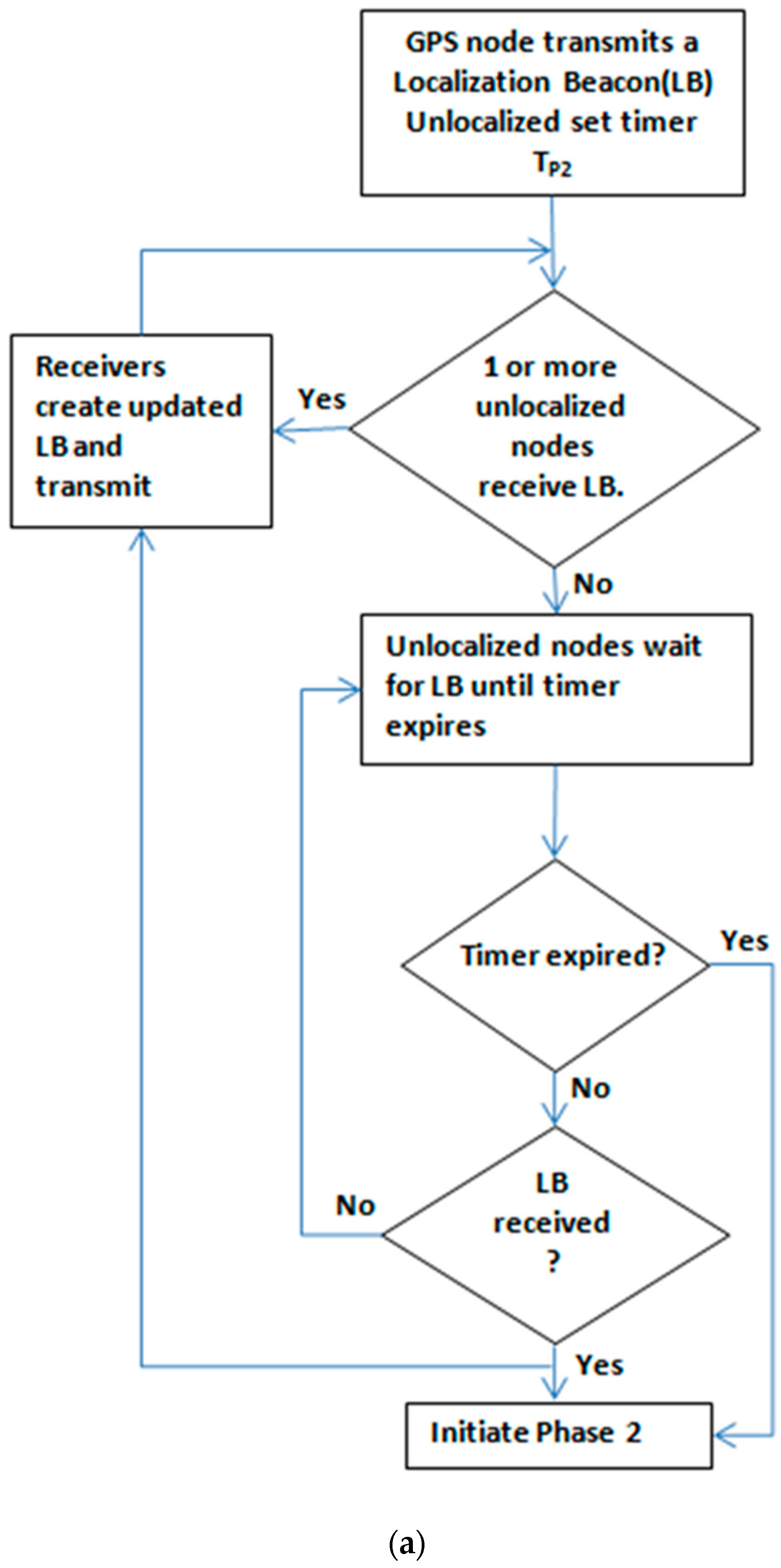
3.2.1. Phase 1: The Reactive Stage
3.2.2. Phase 2: The Proactive stage
Transmission of Localization Requests with Doubled Transmission Range
Clustering and Cluster Head Selection
Reception of Localization Beacon and Retransmission of an Updated Localization Beacon
Cluster Merging
3.2.3. Retransmission Control: Decision Making on the Retransmission of a Received Beacon
3.2.4. Example Scenario
Stage 1: The Reactive Stage
Stage 2: The Proactive Stage
Using TDoA for Localization of Sensor Nodes
4. Simulation Setup
4.1. Energy Consumption Model of Underwater Acoustic Channel
4.2. Parameters Setting
- Nodes are distributed over the simulation area using normal distribution.
- Nodes are distributed in the simulation area in such a way that they form 2 partitions.
- Nodes are distributed in the simulation area in such a way that they form 3 partitions.
- Nodes are distributed in the simulation area in such a way that they form 4 partitions.
5. Results and Discussion
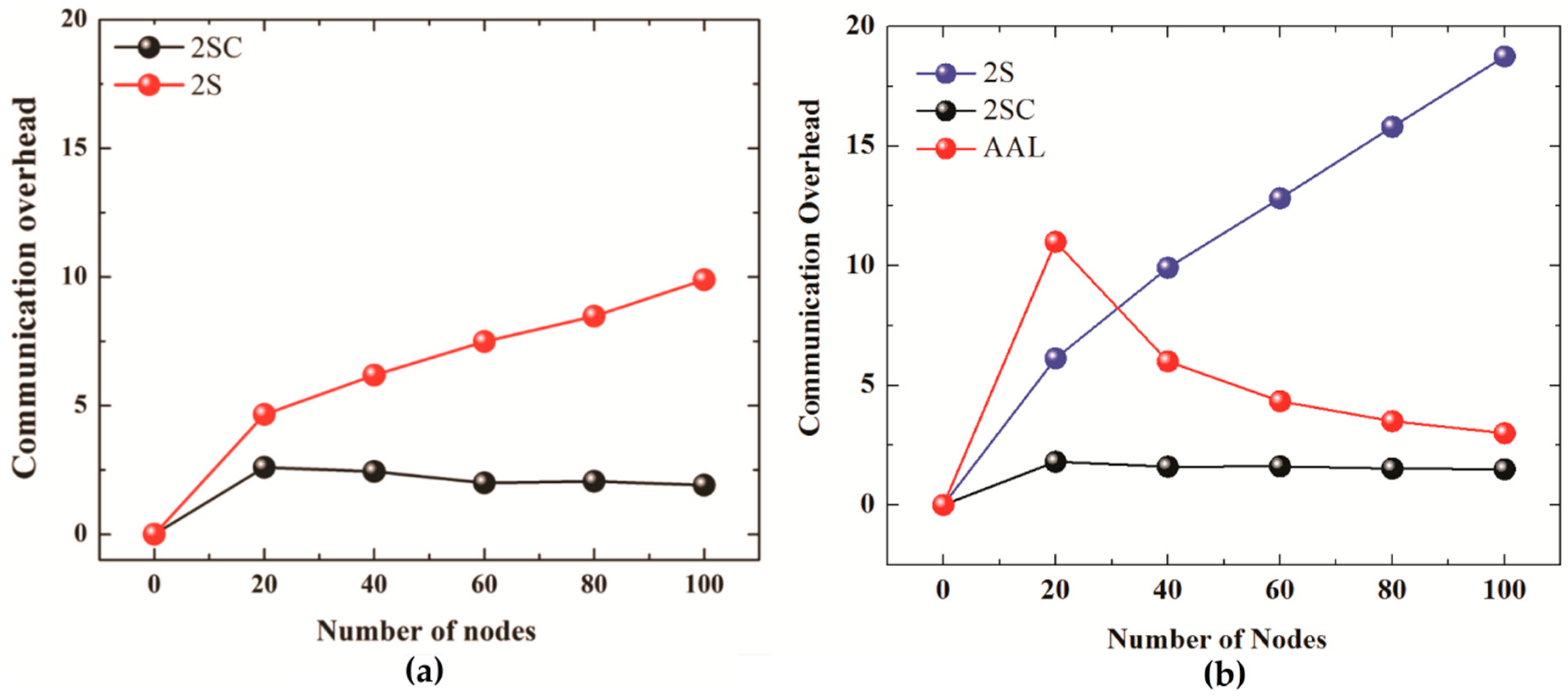
5.1. Communication Overhead
5.2. Energy Consumption
5.3. Localization Error
5.4. Localization Coverage
5.5. Effect of CH Position
- Nearest Case: CH is the nearest node to the GPS node among all the nodes in a cluster.
- Average Case: CH is selected based on value p.
- Farthest Case: CH is the farthest node to the GPS node among all the nodes in a cluster.
5.5.1. Communication Overhead
5.5.2. Energy Consumption
5.5.3. Localization Coverage
6. Conclusions
Author Contributions
Funding
Conflicts of Interest
References
- Felemban, E.; Shaikh, F.K.; Qureshi, U.M.; Sheikh, A.A.; Qaisar, S.B. Underwater sensor network applications: A comprehensive survey. Int. J. Distrib. Sens. Netw. 2015, 11, 896832. [Google Scholar] [CrossRef]
- Tan, H.P.; Diamant, R.; Seah, W.K.; Waldmeyer, M. A survey of techniques and challenges in underwater localization. Ocean Eng. 2011, 38, 1663–1676. [Google Scholar] [CrossRef]
- Bian, T.; Venkatesan, R.; Li, C. Design and evaluation of a new localization scheme for underwater acoustic sensor networks. In Proceedings of the GLOBECOM 2009 Global Telecommunications Conference, Honolulu, HI, USA, 30 November–4 December 2009. [Google Scholar]
- Heidemann, J.; Ye, W.; Wills, J.; Syed, A.; Li, Y. Research challenges and applications for underwater sensor networking. In Proceedings of the Wireless Communications and Networking Conference, Las Vegas, NV, USA, 3–6 April 2006. [Google Scholar]
- Shin, D.-H.; Sung, T.-K. Comparisons of error characteristics between TOA and TDOA positioning. IEEE Trans. Aerosp. Electron. Syst. 2002, 38, 307–311. [Google Scholar] [CrossRef]
- Moradi, M.; Rezazadeh, J.; Ismail, A.S. A reverse localization scheme for underwater acoustic sensor networks. Sensors 2012, 12, 4352–4380. [Google Scholar] [CrossRef] [PubMed]
- Vijay, C.; Seah, W. An area localization scheme for underwater sensor networks. In Proceedings of the OCEANS 2006-Asia Pacific, Singapore, 16–19 May 2006; pp. 1–8. [Google Scholar]
- Cheng, X.; Shu, H.; Liang, Q.; Du, D.H. Silent positioning in underwater acoustic sensor networks. IEEE Trans. Veh. Technol. 2008, 57, 1756–1766. [Google Scholar] [CrossRef]
- Teymorian, A.Y.; Cheng, W.; Ma, L.; Cheng, X.; Lu, X.; Lu, Z. 3D underwater sensor network localization. IEEE Trans. Mob. Comput. 2009, 8, 1610–1621. [Google Scholar] [CrossRef]
- Isik, M.T.; Ozgur, B.A. A three dimensional localization algorithm for underwater acoustic sensor networks. IEEE Trans. Wirel. Commun. 2009, 8, 4457–4463. [Google Scholar] [CrossRef]
- Luo, H.; Guo, Z.; Dong, W.; Hong, F.; Zhao, Y. LDB: Localization with directional beacons for sparse 3D underwater acoustic sensor networks. J. Netw. 2010, 5, 28. [Google Scholar] [CrossRef]
- Zhou, Z.; Peng, Z.; Cui, J.H.; Shi, Z.; Bagtzoglou, A. Scalable localization with mobility prediction for underwater sensor networks. IEEE Trans. Mob. Comput. 2011, 10, 335–348. [Google Scholar] [CrossRef]
- Waldmeyer, M.; Tan, H.-P.; Seah, W.K.G. Multi-stage AUV-aided localization for underwater wireless sensor networks. In Proceedings of the 2011 IEEE Workshops of International Conference on Advanced Information Networking and Applications, Singapore, 22–25 March 2011; pp. 908–913. [Google Scholar]
- Erol, M.; Vieira, L.F.M.; Gerla, M. AUV-aided localization for underwater sensor networks. In Proceedings of the International Conference on Wireless Algorithms, Systems and Applications (WASA2007), Chicago, IL, USA, 1–3 August 2007; pp. 44–54. [Google Scholar]
- Watfa, M.K.; Nsouli, T.; Al-Ayache, M.; Ayyash, O. Reactive localization in underwater wireless sensor networks. In Proceedings of the 2010 Second International Conference on Computer and Network Technology, Bangkok, Thailand, 23–25 April 2010; pp. 244–248. [Google Scholar]
- Luo, J.; Fan, L. A Two-Phase time synchronization-free localization algorithm for underwater sensor networks. Sensors 2017, 17, 726. [Google Scholar] [CrossRef] [PubMed]
- Stojanovic, M. On the relationship between capacity and distance in an underwater acoustic communication channel. ACM Sigmobile Mob. Comput. Commun. Rev. 2007, 11, 34–43. [Google Scholar] [CrossRef]
- Urick, R. Principles of Underwater Sound for Engineers, 3rd ed.; (Reprinted 1996, Peninsula Publ. Los Altos, CA); McGraw-Hill: NewYork, NY, USA, 1983; 423p. [Google Scholar]
- Gao, J. Analysis of energy consumption for adhoc wireless sensor networks using a bit-meter-per-joule metric. IPN Prog. Rep. 2002, 42, 1–19. [Google Scholar]
- Liu, L.; Wu, J.; Zhu, Z. Multihops fitting approach for node localization in underwater wireless sensor networks. Int. J. Distrib. Sens. Netw. 2015, 11, 682182. [Google Scholar] [CrossRef]
- Evo Logics. Available online: https://www.evologics.de/en/products/acoustics/s2cr_48_78.html (accessed on 27 February 2019).


| Parameters | Values |
|---|---|
| Deployment area | 1000 m × 1000 m |
| Default range | 150 m |
| Number of nodes | 20, 40, 60, 80, 100 |
| Number of partitions | 1, 2, 3, 4 |
| Packet size | 512 bits |
| Data rate | 5000 bps |
| Error in speed of sound | 0.2 m/s [20] |
| Depth error | 0.1 m [20] |
| Error due to node mobility | 0.1 [20] |
| Anchor node positioning error | ±1 m |
| AUV positioning error | ±1 m [14] |
| Total length of AUV spiral path | 5000 m |
| AUV beacon transmission | 50 m |
| Simulation Runs | 100 |
| Energy Consumption (W) | Range (m) |
|---|---|
| 5.5 | 250 |
| 8 | 500 |
| 18 | 1000 |
| 60 | Above 1000 |
© 2019 by the authors. Licensee MDPI, Basel, Switzerland. This article is an open access article distributed under the terms and conditions of the Creative Commons Attribution (CC BY) license (http://creativecommons.org/licenses/by/4.0/).
Share and Cite
Islam, T.; Lee, Y.K. A Cluster Based Localization Scheme with Partition Handling for Mobile Underwater Acoustic Sensor Networks. Sensors 2019, 19, 1039. https://doi.org/10.3390/s19051039
Islam T, Lee YK. A Cluster Based Localization Scheme with Partition Handling for Mobile Underwater Acoustic Sensor Networks. Sensors. 2019; 19(5):1039. https://doi.org/10.3390/s19051039
Chicago/Turabian StyleIslam, Tariq, and Yong Kyu Lee. 2019. "A Cluster Based Localization Scheme with Partition Handling for Mobile Underwater Acoustic Sensor Networks" Sensors 19, no. 5: 1039. https://doi.org/10.3390/s19051039
APA StyleIslam, T., & Lee, Y. K. (2019). A Cluster Based Localization Scheme with Partition Handling for Mobile Underwater Acoustic Sensor Networks. Sensors, 19(5), 1039. https://doi.org/10.3390/s19051039