Estimating Visibility of Annotations for View Management in Spatial Augmented Reality Based on Machine-Learning Techniques


Abstract
:1. Introduction
- Supervised machine learning-based view management method for spatial AR is proposed and implemented.
- A user friendly visibility is defined that reflects human’s subjective mental workload in reading projected information as well as objective measures in corectness of reading.
- Visibility classification features are proposed that represent reflective characteristics of the projection surface, the three dimensional properties of physical objects on the projection surface, and the spatial relationship between the objects, the projector-camera systems, and the user’s viewpoint.
- Feature subset is identified that improves processing speed up to 170% with slight degradation of classification performance.
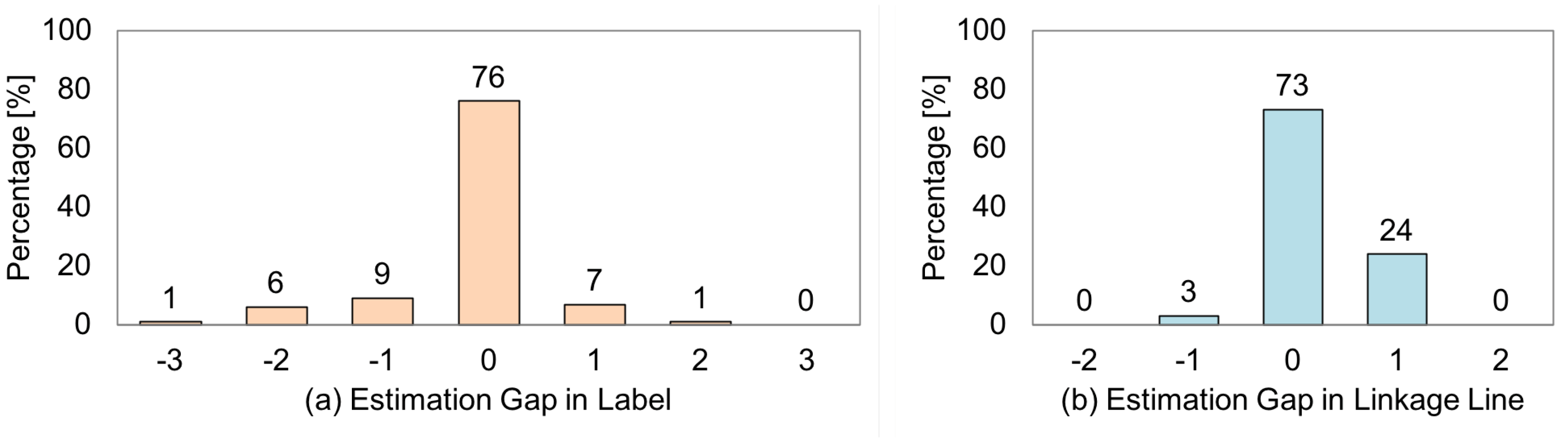
- An online experiment with new users and objects showed that 76.0% of the system’s judgments were matched with the users’ evaluations, while 73% of the linkage line visibility estimations were matched.
2. Related Work
2.1. Mediation of Reality
2.2. View Management Method
2.2.1. Geometric-Based Layout
2.2.2. Image-Based Layout
3. Overview of Visibility-Aware Label Placement System
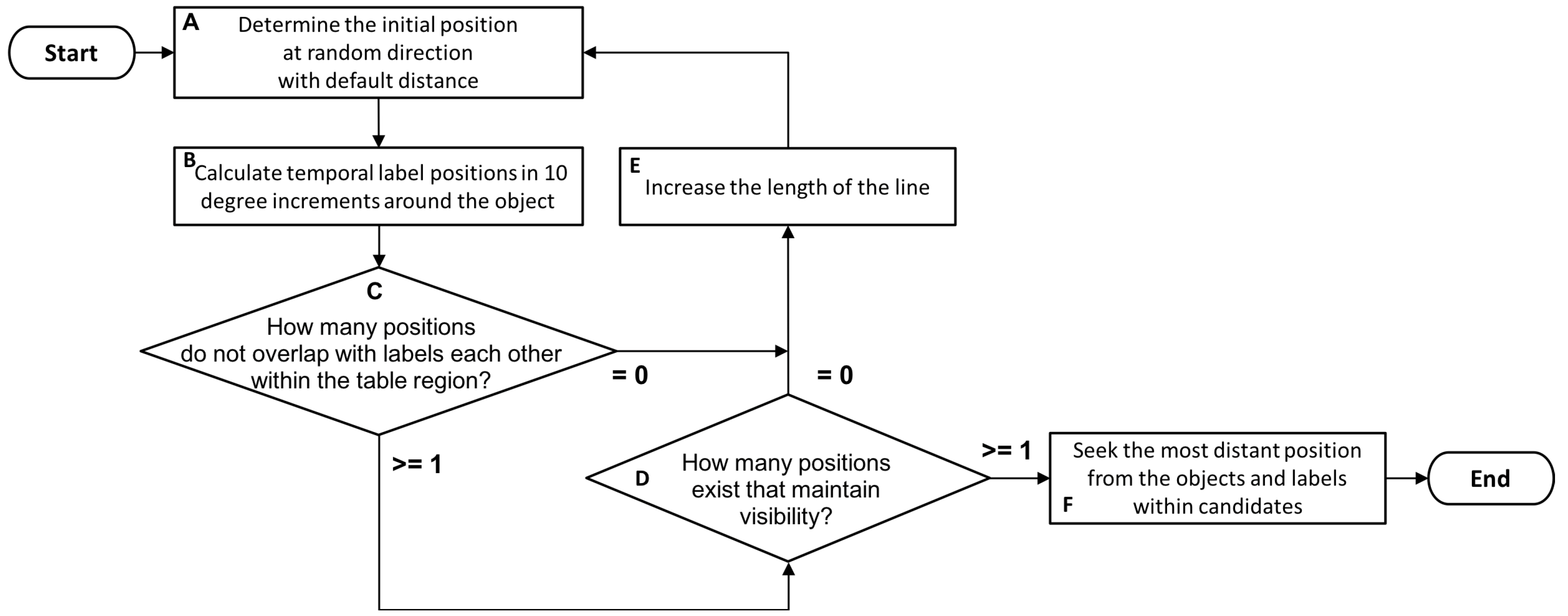
3.1. VisLP Algorithm
3.2. Problem Definition
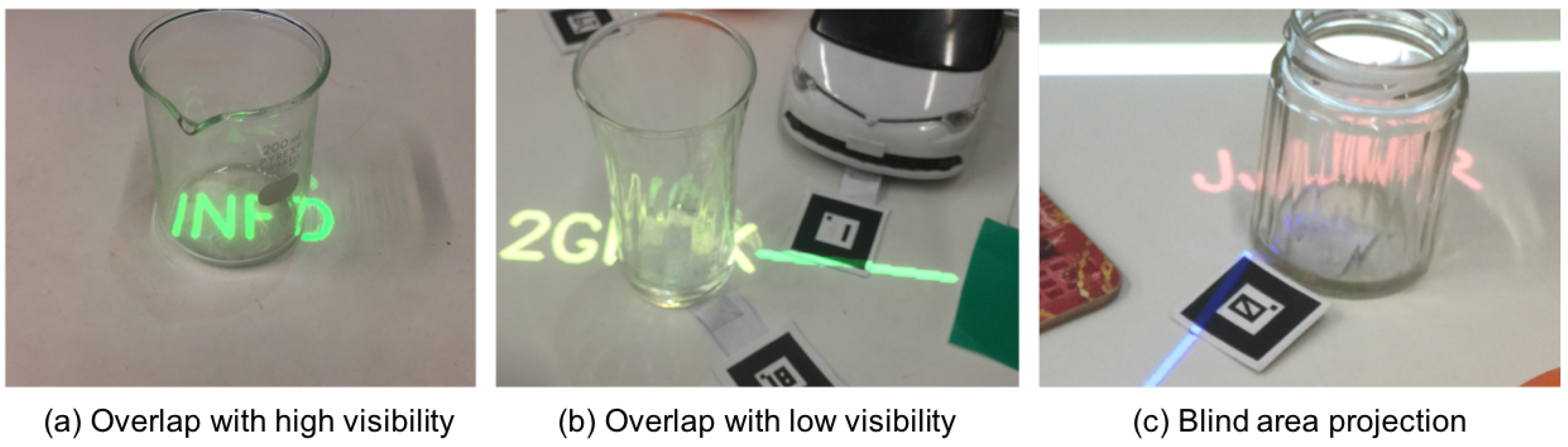
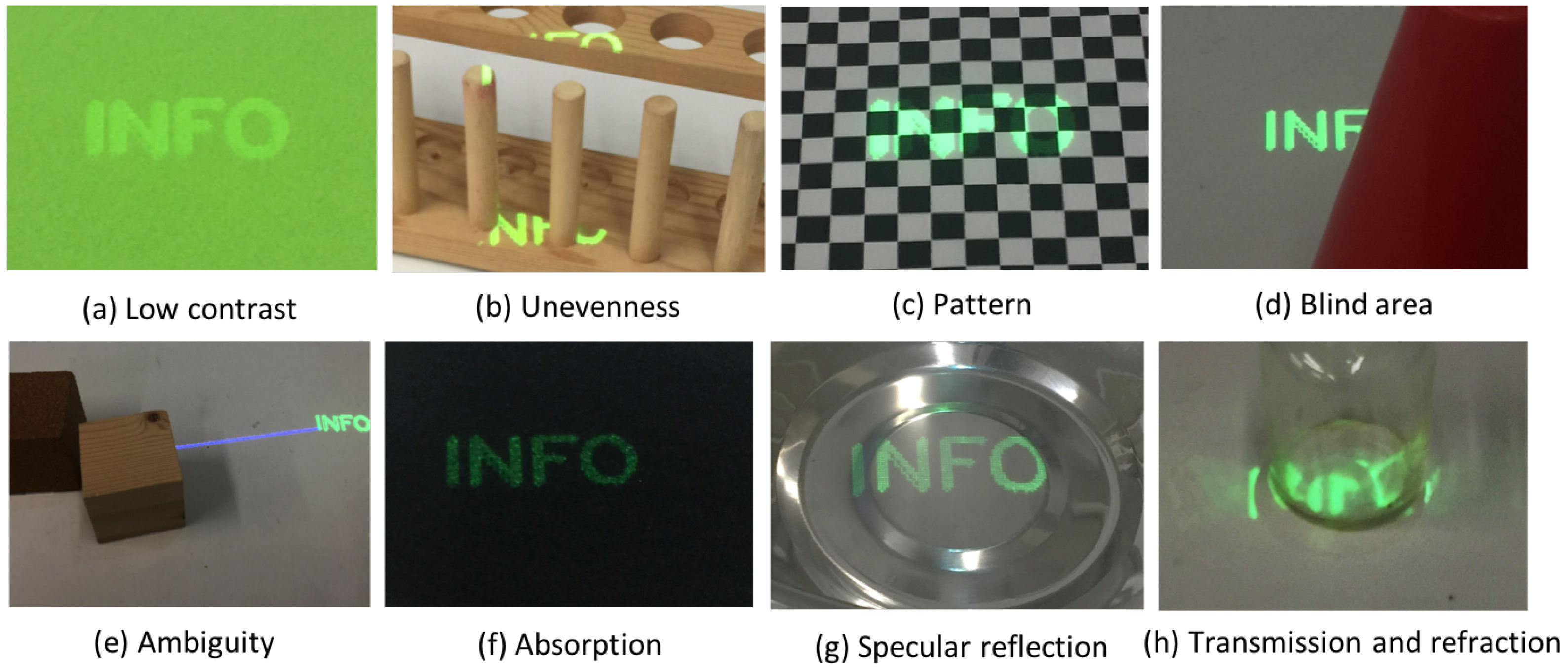
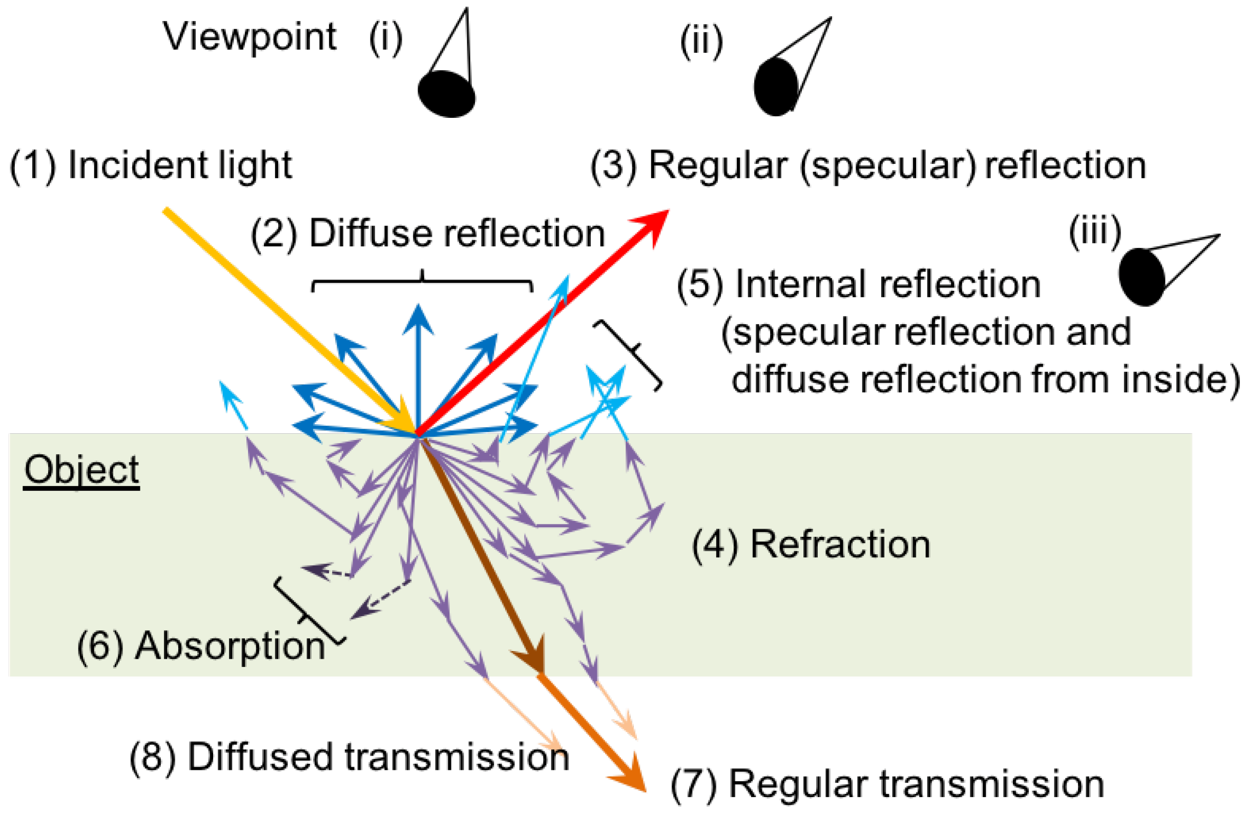
3.3. Factors that Degrade Visibility
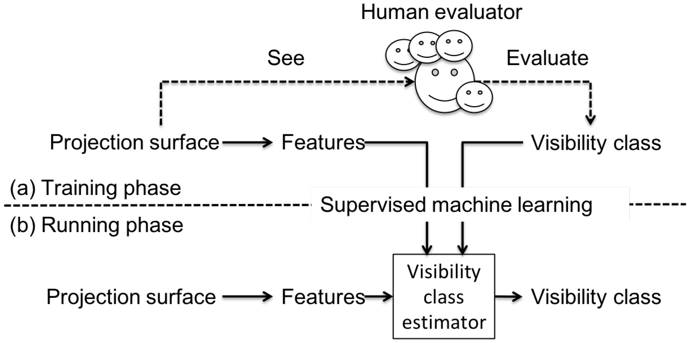
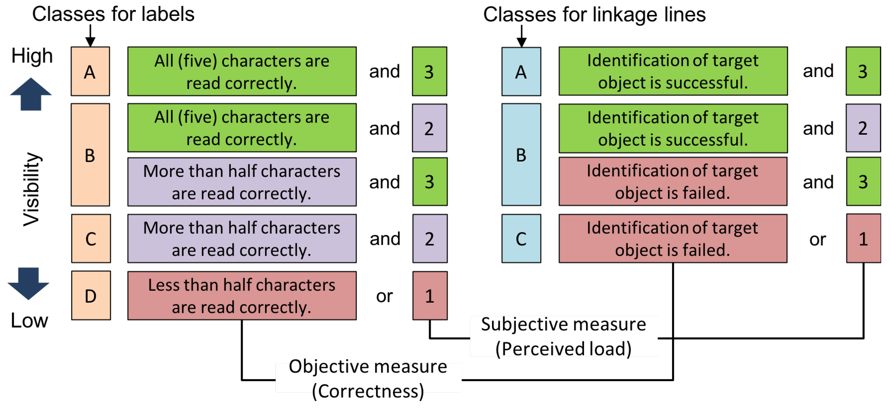
3.4. Visibility Classes
4. Designing Features for Visibility Estimation
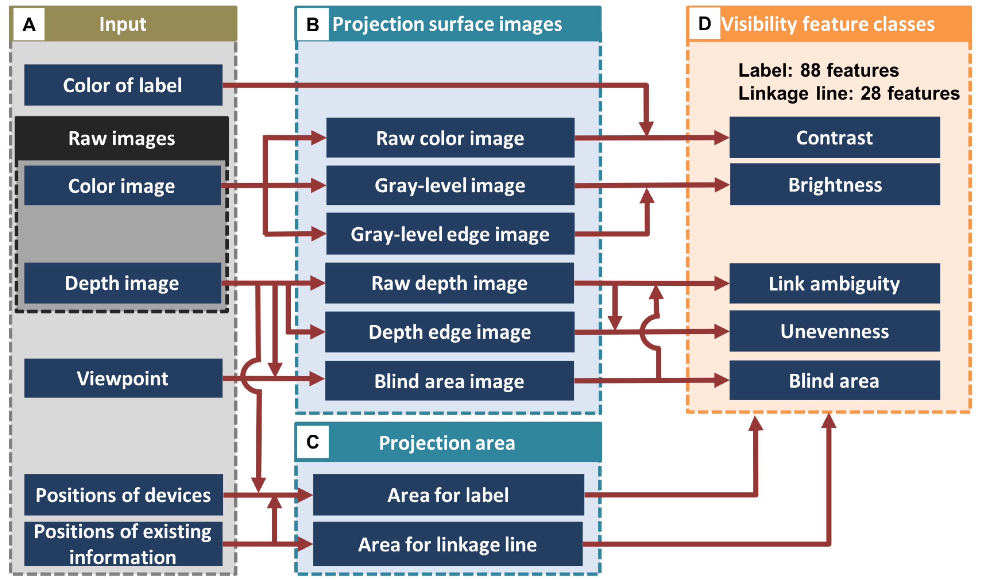
4.1. Basic Flow of Feature Calculation
4.1.1. Input
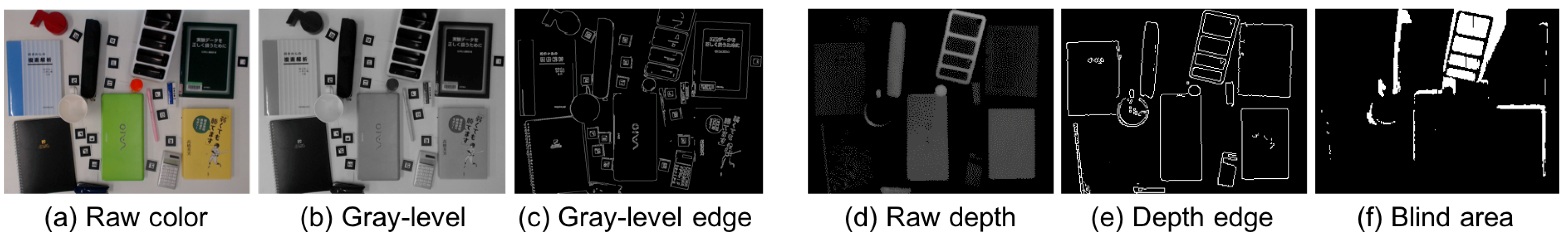
4.1.2. Projection Surface Images
4.1.3. Projection Area
4.1.4. Visibility Feature Classes
4.2. Definition of the Features for a Label
4.2.1. Contrast Features
4.2.2. Brightness Features
4.2.3. Unevenness Features
4.2.4. Blind Area Feature
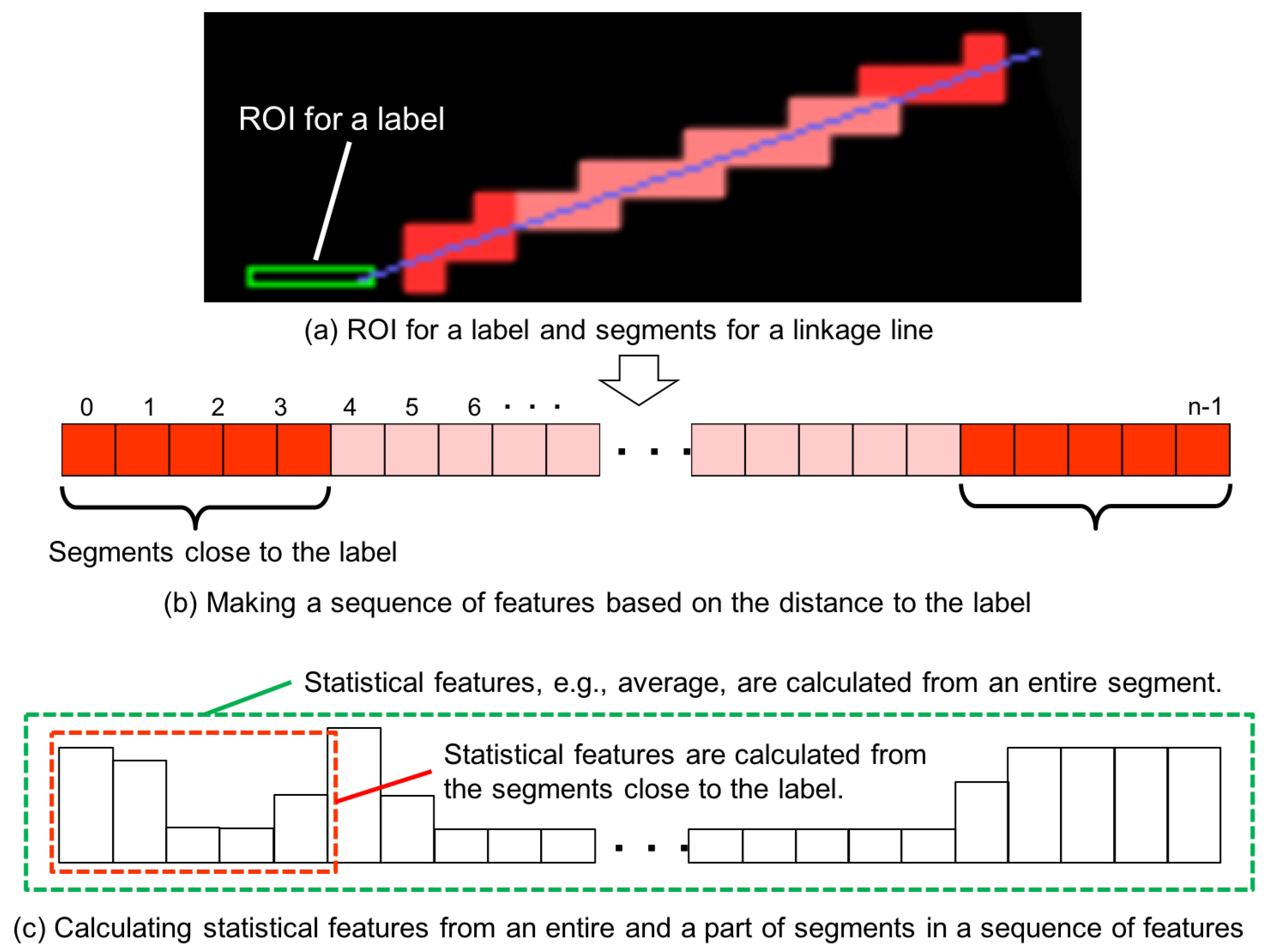
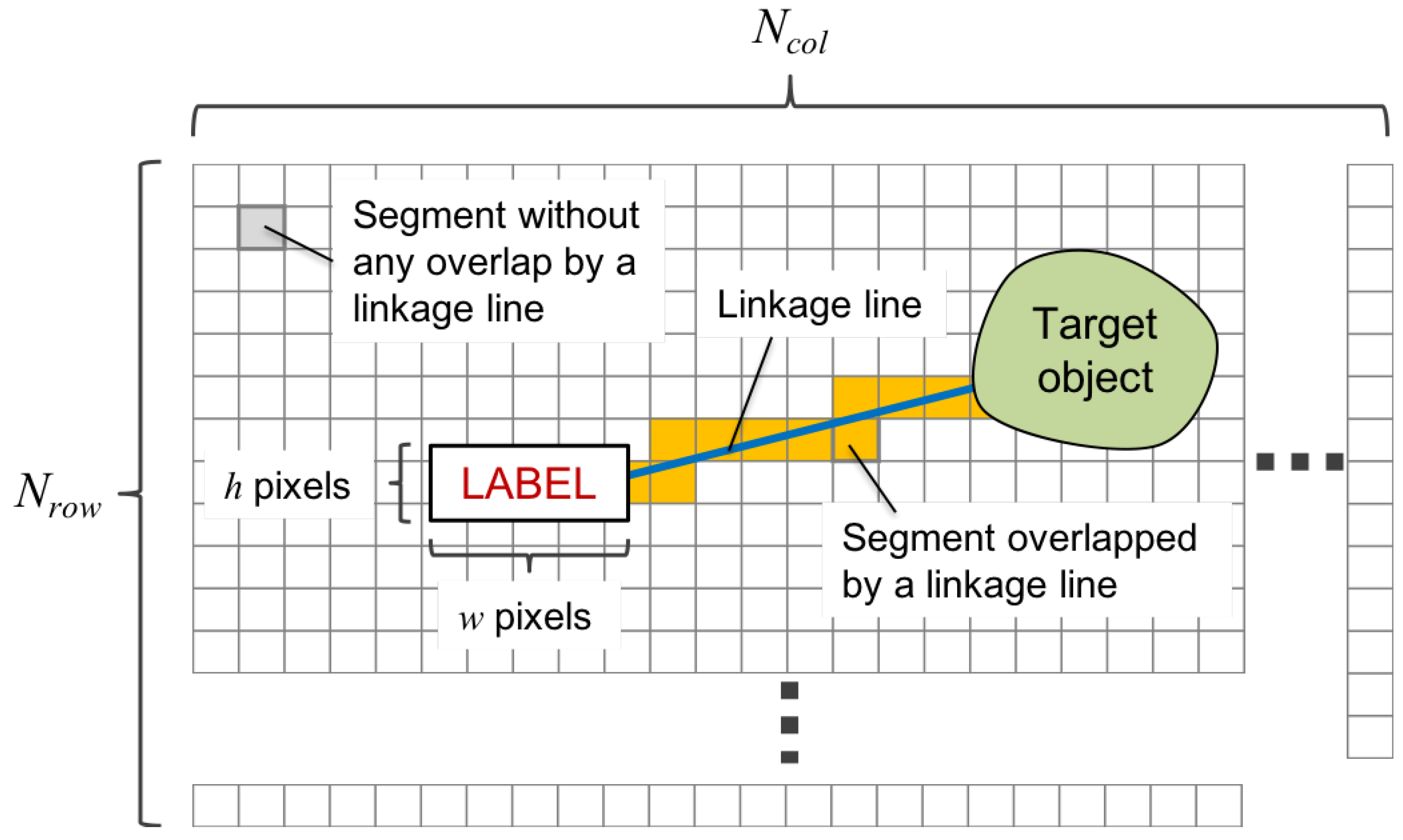
4.3. Definition of Features for a Linkage Line
- Step 1:
- Calculation of segment features
- Step 2:
- Making a sequence of segment features
- Step 3:
- Calculation of the linkage line features from the sequence data
5. Dataset for Training and Testing Visibility Estimator
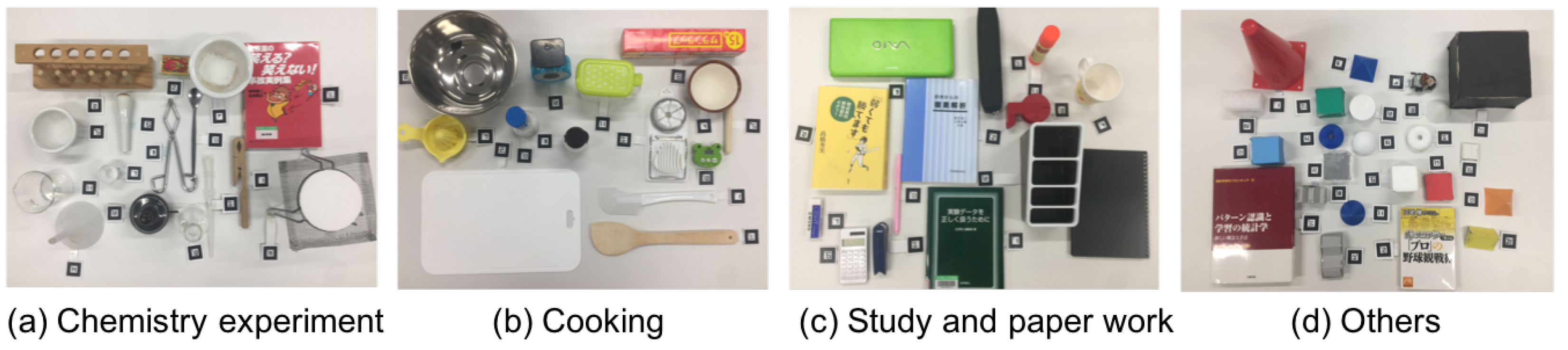
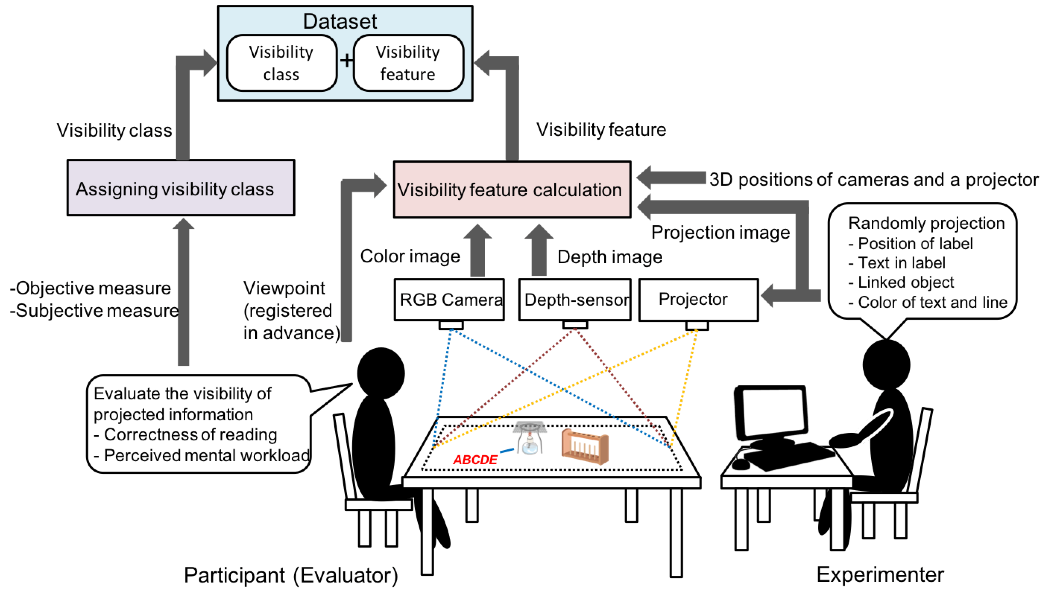
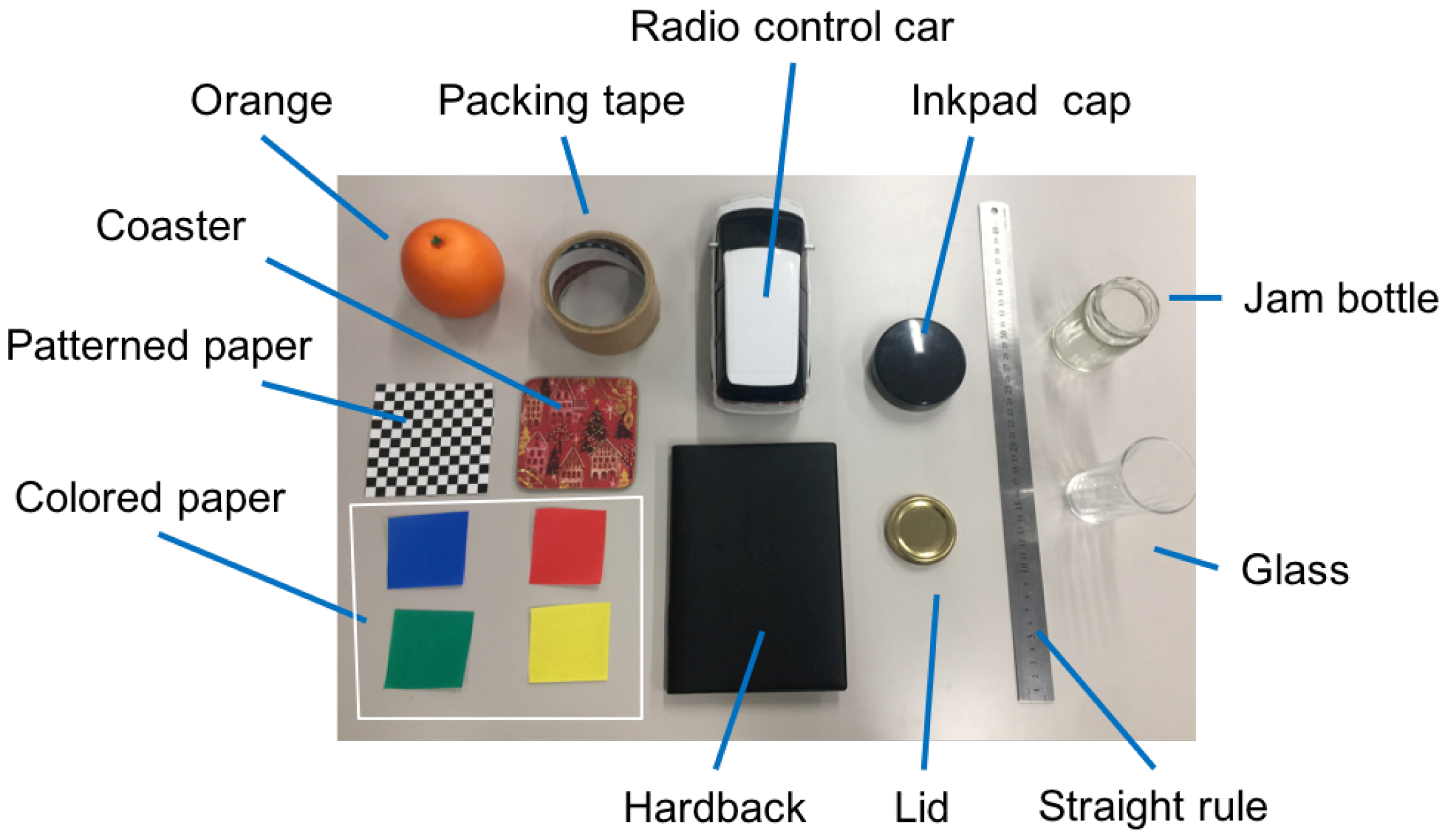
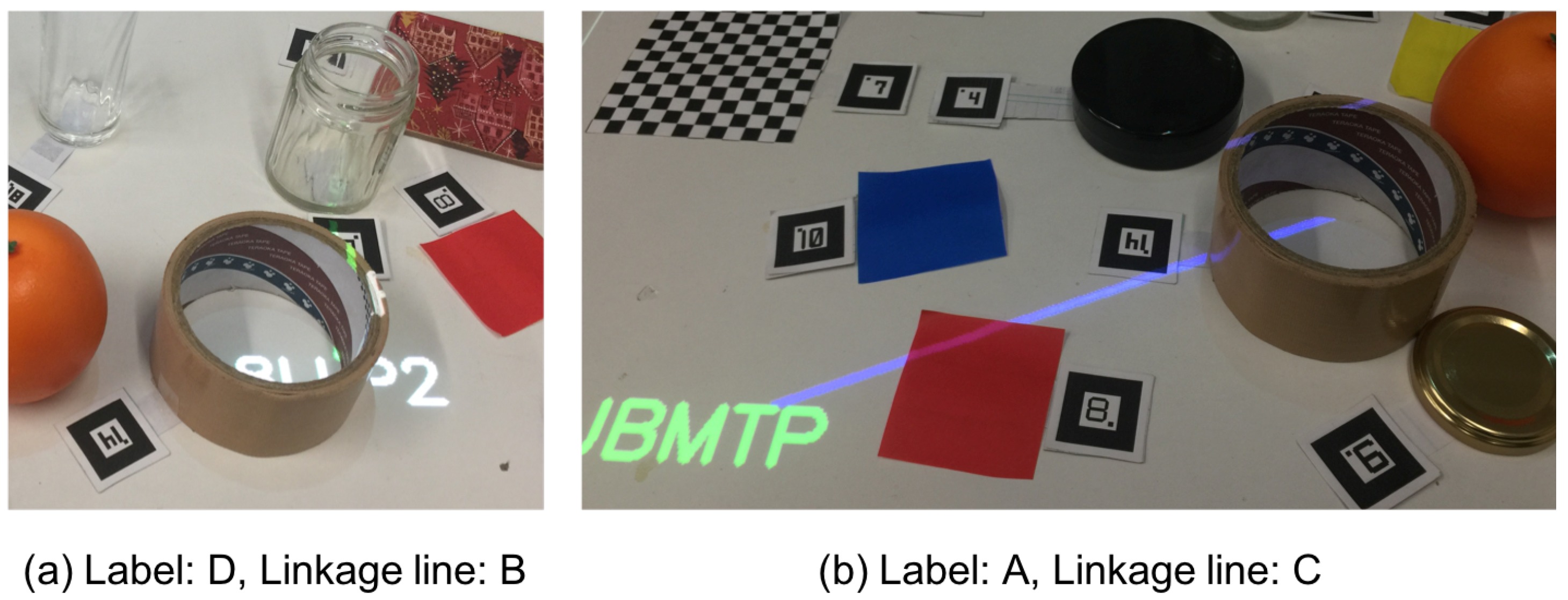
5.1. Data Collection
5.2. Data Augmentation for Balanced Dataset
6. Evaluation
6.1. Difference in Various Models of Classifiers
6.1.1. Methodology
6.1.2. Result
6.2. Feature Subset Evaluation
6.2.1. Methodology
6.2.2. Results and Discussion
6.3. Online Experiment with Users
6.3.1. Methodology
6.3.2. Results and Discussion
7. Conclusions
Author Contributions
Funding
Conflicts of Interest
References
- Azuma, R.T. A Survey of Augmented Reality. Presence Teleoper. Virtual Environ. 1997, 6, 355–385. [Google Scholar] [CrossRef]
- Bimber, O.; Raskar, R. Spatial Augmented Reality: Merging Real and Virtual Worlds; A K Peters, Ltd.: Natick, MA, USA, 2005. [Google Scholar]
- Suzuki, Y.; Morioka, S.; Ueda, H. Cooking Support with Information Projection Onto Ingredient. In Proceedings of the 10th Asia Pacific Conference on Computer Human Interaction, Shimane, Japan, 28–31 August 2012; ACM: New York, NY, USA, 2012; pp. 193–198. [Google Scholar] [CrossRef]
- Suzuki, K.; Fujinami, K. A Projector-Camera System for Ironing Support with Wrinkle Enhancement. ICST Trans. Ambient Syst. 2017, 4, 153047. [Google Scholar] [CrossRef]
- Funk, M.; Shirazi, A.S.; Mayer, S.; Lischke, L.; Schmidt, A. Pick from here!—An Interactive Mobile Cart using In-Situ Projection for Order Picking. In Proceedings of the 2015 ACM International Joint Conference on Pervasive and Ubiquitous Computing—UbiComp ’15, Osaka, Japan, 7–11 September 2015; ACM Press: New York, NY, USA, 2015; pp. 601–609. [Google Scholar] [CrossRef]
- Doshi, A.; Smith, R.T.; Thomas, B.H.; Bouras, C. Use of projector based augmented reality to improve manual spot-welding precision and accuracy for automotive manufacturing. Int. J. Adv. Manuf. Technol. 2017, 89, 1279–1293. [Google Scholar] [CrossRef]
- Uva, A.E.; Gattullo, M.; Manghisi, V.M.; Spagnulo, D.; Cascella, G.L.; Fiorentino, M. Evaluating the effectiveness of spatial augmented reality in smart manufacturing: A solution for manual working stations. Int. J. Adv. Manuf. Technol. 2018, 94, 509–521. [Google Scholar] [CrossRef]
- Joo-Nagata, J.; Martinez Abad, F.; García-Bermejo Giner, J.; García-Peñalvo, F.J. Augmented reality and pedestrian navigation through its implementation in m-learning and e-learning: Evaluation of an educational program in Chile. Comput. Educ. 2017, 111, 1–17. [Google Scholar] [CrossRef]
- Sokan, A.; Hou, M.; Shinagawa, N.; Egi, H.; Fujinami, K. A Tangible Experiment Support System with Presentation Ambiguity for Safe and Independent Chemistry Experiments. J. Ambient Intell. Humaniz. Comput. 2012, 3, 125–139. [Google Scholar] [CrossRef]
- Cascales-Martínez, A. Using an Augmented Reality Enhanced Tabletop System to Promote Learning of Mathematics: A Case Study with Students with Special Educational Needs. EURASIA J. Math. Sci. Technol. Educ. 2017, 13, 355–380. [Google Scholar] [CrossRef]
- Iwai, D.; Yabiki, T.; Sato, K. View Management of Projected Labels on Nonplanar and Textured Surfaces. IEEE Trans. Vis. Comput. Graph. 2013, 19, 1415–1424. [Google Scholar] [CrossRef] [PubMed]
- Murata, S.; Suzuki, M.; Fujinami, K. A Wearable Projector-based Gait Assistance System and Its Application for Elderly People. In Proceedings of the 2013 ACM International Joint Conference on Pervasive and Ubiquitous Computing, Zurich, Switzerland, 8–12 September 2013; ACM: New York, NY, USA, 2013; pp. 143–152. [Google Scholar] [CrossRef]
- Amano, T.; Kato, H. Appearance control by projector camera feedback for visually impaired. In Proceedings of the 2010 IEEE Computer Society Conference on Computer Vision and Pattern Recognition-Workshops, San Francisco, CA, USA, 13–18 June 2010; pp. 57–63. [Google Scholar] [CrossRef]
- Tanaka, N.; Fujinami, K. A Projector-Camera System for Augmented Card Playing and a Case Study with the Pelmanism Game. ICST Trans. Ambient Syst. 2017, 4, 152550. [Google Scholar] [CrossRef]
- Azuma, R.; Furmanski, C. Evaluating Label Placement for Augmented Reality View Management. In Proceedings of the 2nd IEEE/ACM International Symposium on Mixed and Augmented Reality; IEEE Computer Society: Washington, DC, USA, 2003; pp. 66–75. [Google Scholar]
- Bell, B.; Feiner, S.; Höllerer, T. View Management for Virtual and Augmented Reality. In Proceedings of the 14th Annual ACM Symposium on User Interface Software and Technology, Orlando, FL, USA, 11–14 November 2001; ACM: New York, NY, USA, 2001; pp. 101–110. [Google Scholar] [CrossRef]
- Scharff, L.F.; Hill, A.L.; Ahumada, A.J. Discriminability measures for predicting readability of text on textured backgrounds. Opt. Express 2000, 6, 81–91. [Google Scholar] [CrossRef] [PubMed]
- Gabbard, J.L.; Swan, J.E.; Hix, D. The Effects of Text Drawing Styles, Background Textures, and Natural Lighting on Text Legibility in Outdoor Augmented Reality. Presence Teleoper. Virtual Environ. 2006, 15, 16–32. [Google Scholar] [CrossRef]
- Orlosky, J.; Kiyokawa, K.; Takemura, H. Managing mobile text in head mounted displays: Studies on visual preference and text placement. ACM SIGMOBILE Mob. Comput. Commun. Rev. 2014, 18, 20–31. [Google Scholar] [CrossRef]
- Makita, K.; Kanbara, M.; Yokoya, N. View management of annotations for wearable augmented reality. In Proceedings of the 2009 IEEE International Conference on Multimedia and Expo, New York, NY, USA, 28 June–3 July 2009; pp. 982–985. [Google Scholar] [CrossRef]
- Sato, M.; Fujinami, K. Nonoverlapped view management for augmented reality by tabletop projection. J. Vis. Lang. Comput. 2014, 25, 891–902. [Google Scholar] [CrossRef]
- Kohei Tanaka, K.; Kishino, Y.; Miyamae, M.; Terada, T.; Nishio, S. An information layout method for an optical see-through head mounted display focusing on the viewability. In Proceedings of the 2008 7th IEEE/ACM International Symposium on Mixed and Augmented Reality, Cambridge, UK, 15–18 September 2008; pp. 139–142. [Google Scholar] [CrossRef]
- Imhof, E. Positioning Names on Maps. Am. Cartogr. 1975, 2, 128–144. [Google Scholar] [CrossRef]
- Di Donato, M.; Fiorentino, M.; Uva, A.E.; Gattullo, M.; Monno, G. Text legibility for projected Augmented Reality on industrial workbenches. Comput. Ind. 2015, 70, 70–78. [Google Scholar] [CrossRef]
- Mann, S. Mediated Reality with Implementations for Everyday Life. 2002. Available online: http://wearcam.org/presence_connect/ (accessed on 31 January 2019).
- Mori, S.; Ikeda, S.; Saito, H. A survey of diminished reality: Techniques for visually concealing, eliminating, and seeing through real objects. IPSJ Trans. Comput. Vis. Appl. 2017, 9, 17. [Google Scholar] [CrossRef]
- Shibata, F.; Nakamoto, H.; Sasaki, R.; Kimura, A.; Tamura, H. A View Management Method for Mobile Mixed Reality Systems. In Proceedings of the 14th Eurographics Conference on Virtual Environments, Eindhoven, The Netherlands, 29–30 May 2008; Eurographics Association: Aire-la-Ville, Switzerland, 2008; pp. 17–24. [Google Scholar] [CrossRef]
- Leykin, A.; Tuceryan, M. Automatic determination of text readability over textured backgrounds for augmented reality systems. In Proceedings of the 3rd IEEE/ACM International Symposium on Mixed and Augmented Reality Systems, Arlington, VA, USA, 2–4 November 2004; pp. 224–230. [Google Scholar]
- Achanta, R.; Hemami, S.; Estrada, F.; Susstrunk, S. Frequency-tuned salient region detection. In Proceedings of the 2009 IEEE Conference on Computer Vision and Pattern Recognition, Miami, FL, USA, 22–25 June 2009; pp. 1597–1604. [Google Scholar] [CrossRef]
- Chang, M.M.L.; Ong, S.K.; Nee, A.Y.C. Automatic Information Positioning Scheme in AR-assisted Maintenance Based on Visual Saliency; Springer: Cham, Switzerland, 2016; pp. 453–462. [Google Scholar] [CrossRef]
- Ens, B.M.; Finnegan, R.; Irani, P.P. The personal cockpit: A spatial interface for effective task switching on head-worn. In Proceedings of the 32nd Annual ACM conference on Human factors in Computing Systems–CHI’14, Toronto, ON, Canada, 26 April–1 May 2014; ACM Press: New York, NY, USA, 2014; pp. 3171–3180. [Google Scholar] [CrossRef]
- Li, G.; Liu, Y.; Wang, Y.; Xu, Z. Evaluation of labelling layout method for image-driven view management in augmented reality. In Proceedings of the 29th Australian Conference on Computer-Human Interaction—OZCHI ’17, Brisbane, Australia, 28 November–1 December 2017; ACM Press: New York, NY, USA, 2017; pp. 266–274. [Google Scholar] [CrossRef]
- Grasset, R.; Langlotz, T.; Kalkofen, D.; Tatzgern, M.; Schmalstieg, D. Image-driven View Management for Augmented Reality Browsers. In Proceedings of the 2012 IEEE International Symposium on Mixed and Augmented Reality (ISMAR), Atlanta, GA, USA, 5–8 November 2012; IEEE Computer Society: Washington, DC, USA, 2012; pp. 177–186. [Google Scholar] [CrossRef]
- Siriborvornratanakul, T.; Sugimoto, M. Clutter-aware Adaptive Projection Inside a Dynamic Environment. In Proceedings of the 2008 ACM Symposium on Virtual Reality Software and Technology, Bordeaux, France, 27–29 October 2008; ACM: New York, NY, USA, 2008; pp. 241–242. [Google Scholar] [CrossRef]
- Riemann, J.; Khalilbeigi, M.; Schmitz, M.; Doeweling, S.; Müller, F.; Mühlhäuser, M. FreeTop: Finding Free Spots for Projective Augmentation. In Proceedings of the 2016 CHI Conference Extended Abstracts on Human Factors in Computing Systems—CHI EA ’16, San Jose, CA, USA, 7–12 May 2016; ACM Press: New York, NY, USA, 2016; pp. 1598–1606. [Google Scholar] [CrossRef]
- Cotting, D.; Gross, M. Interactive environment-aware display bubbles. In Proceedings of the 19th Annual ACM Symposium on User Interface Software and Technology—UIST ’06, Montreux, Switzerland, 15–18 October 2006; ACM Press: New York, NY, USA, 2006; p. 245. [Google Scholar] [CrossRef]
- Canny, J. A Computational Approach to Edge Detection. IEEE Trans. Pattern Anal. Mach. Intell. 1986, PAMI-8, 679–698. [Google Scholar] [CrossRef]
- Blinn, J. Me and My (Fake) Shadow. IEEE Comput. Graph. Appl. 1988, 8, 82–86. [Google Scholar]
- W3C/WAI. Techniques for Accessibility Evaluation and Repair Tools. 2000. Available online: https://www.w3.org/WAI/ER/WD-AERT/ (accessed on 31 December 2018).
- Motoyoshi, I. Perception of Shitsukan: Visual Perception of Surface Qualities and Materials. J. Inst. Image Inf. Telev. Eng. 2012, 66, 338–342. [Google Scholar] [CrossRef]
- Chaudhuri, B.; Sarkar, N. Texture segmentation using fractal dimension. IEEE Trans. Pattern Anal. Mach. Intell. 1995, 17, 72–77. [Google Scholar] [CrossRef]
- Lin, K.H.; Lam, K.M.; Siu, W.C. Locating the eye in human face images using fractal dimensions. IEE Proc. Vis. Image Signal Process. 2001, 148, 413–421. [Google Scholar] [CrossRef]
- Ida, T.; Sambonsugi, Y. Image segmentation and contour detection using fractal coding. IEEE Trans. Circuits Syst. Video Technol. 1998, 8, 968–975. [Google Scholar] [CrossRef]
- Neil, G.; Curtis, K. Shape recognition using fractal geometry. Pattern Recognit. 1997, 30, 1957–1969. [Google Scholar] [CrossRef]
- Peitgen, H.O.; Jürgens, H.; Saupe, D. Chaos and Fractals, 2nd ed.; Springer: New York, NY, USA, 2004. [Google Scholar] [CrossRef]
- Haralick, R.M.; Shanmugam, K.; Dinstein, I. Textural Features for Image Classification. IEEE Trans. Syst. Man Cybern. 1973, 3, 610–621. [Google Scholar] [CrossRef]
- Galloway, M.M. Texture analysis using gray level run lengths. Comput. Graphics Image Process. 1975, 4, 172–179. [Google Scholar] [CrossRef]
- Machine Learning Group at University of Waikato. Weka 3—Data Mining with Open Source Machine Learning Software in Java. 2017. Available online: http://www.cs.waikato.ac.nz/ml/weka/ (accessed on 31 December 2018).
- Witten, I.H.; Frank, E.; Hall, M.A. Data Mining: Practical Machine Learning Tools and Techniques, 3rd ed.; Morgan Kaufmann Publishers: San Francisco, CA, USA, 2011. [Google Scholar]


| Score | Criteria for a Label | Criteria for a Linkage Line |
|---|---|---|
| 1 | I cannot understand more than half of the characters. | I cannot identify the target object. |
| 2 | I can understand a couple of characters, | I am not confident of the target object |
| or it takes some time to understand all characters. | although I think I can identify it, | |
| or it takes some time to identify the target. | ||
| 3 | I can understand all characters immediately. | I can identify the target object immediately. |
| Type | Label | Linkage Line | |||||
|---|---|---|---|---|---|---|---|
| Class | A | B | C | D | A | B | C |
| Number of samples (Original) | 5712 | 2349 | 1868 | 2071 | 8816 | 2663 | 521 |
| Number of samples (Balanced) | 2500 | 2500 | 2500 | 2500 | 600 | 600 | 600 |
| RF | SVM | NN | NB |
|---|---|---|---|
| 0.919 | 0.912 | 0.911 | 0.530 |
| Classified as | Recall | |||||
|---|---|---|---|---|---|---|
| A | B | C | D | |||
| Original | A | 2360 | 19 | 116 | 5 | 0.944 |
| B | 46 | 2258 | 95 | 101 | 0.903 | |
| C | 133 | 134 | 2211 | 22 | 0.884 | |
| D | 20 | 99 | 22 | 2359 | 0.944 | |
| Precision | 0.922 | 0.900 | 0.905 | 0.949 | F: 0.919 | |
| Segment Resolution () | RF | SVM | NN | NB |
|---|---|---|---|---|
| 72 × 96 | 0.782 | 0.742 | 0.705 | 0.539 |
| 36 × 48 | 0.789 | 0.732 | 0.721 | 0.559 |
| 24 × 32 | 0.774 | 0.702 | 0.700 | 0.547 |
| 18 × 24 | 0.745 | 0.721 | 0.708 | 0.553 |
| Classified as | Recall | ||||
|---|---|---|---|---|---|
| A | B | C | |||
| Original | A | 485 | 57 | 58 | 0.808 |
| B | 76 | 453 | 71 | 0.755 | |
| C | 58 | 60 | 482 | 0.803 | |
| Precision | 0.784 | 0.795 | 0.789 | F: 0.789 | |
| Name | Type | Sel. | IG [bit] | Name | Type | Sel. | IG [bit] | Name | Type | Sel. | IG [bit] |
|---|---|---|---|---|---|---|---|---|---|---|---|
| BR | BA | ✓ | 0.737 | UE | 0.312 | BR | 0.184 | ||||
| UE | 0.469 | UE | 0.307 | BR | 0.184 | ||||||
| UE | 0.451 | UE | 0.304 | BR | 0.183 | ||||||
| BR | ✓ | 0.448 | UE | 0.302 | BR | 0.176 | |||||
| BR | 0.447 | UE | 0.300 | BR | ✓ | 0.164 | |||||
| BR | 0.446 | UE | 0.298 | BR | 0.147 | ||||||
| BR | ✓ | 0.439 | BR | 0.285 | BR | 0.142 | |||||
| UE | ✓ | 0.438 | BR | 0.283 | BR | 0.141 | |||||
| UE | ✓ | 0.438 | BR | 0.278 | BR | 0.140 | |||||
| BR | ✓ | 0.435 | UE | 0.277 | BR | 0.139 | |||||
| BR | 0.435 | UE | 0.273 | BR | 0.136 | ||||||
| UE | 0.410 | UE | 0.269 | BR | 0.135 | ||||||
| UE | ✓ | 0.408 | UE | 0.264 | BR | ✓ | 0.127 | ||||
| UE | 0.402 | BR | 0.259 | BR | 0.125 | ||||||
| UE | 0.392 | UE | 0.255 | BR | 0.123 | ||||||
| BR | 0.392 | UE | 0.253 | BR | 0.107 | ||||||
| BR | 0.390 | UE | 0.248 | BR | 0.105 | ||||||
| UE | 0.378 | UE | 0.247 | BR | 0.103 | ||||||
| UE | 0.376 | BR | ✓ | 0.239 | BR | 0.079 | |||||
| UE | 0.375 | UE | ✓ | 0.237 | BR | ✓ | 0.053 | ||||
| BR | 0.371 | BR | 0.233 | BR | 0.052 | ||||||
| UE | 0.360 | UE | ✓ | 0.233 | BR | 0.052 | |||||
| UE | 0.359 | UE | 0.221 | BR | 0.049 | ||||||
| UE | ✓ | 0.347 | UE | 0.219 | BR | 0.048 | |||||
| BR | ✓ | 0.344 | UE | 0.216 | BR | 0.047 | |||||
| UE | 0.342 | UE | 0.216 | BR | 0.046 | ||||||
| BR | 0.333 | UE | 0.209 | CN | 0.013 | ||||||
| UE | 0.331 | BR | 0.197 | CN | 0.009 | ||||||
| BR | 0.326 | UE | 0.187 | ||||||||
| UE | 0.317 | UE | 0.184 |
| Name | Type | Sel. | IG [bit] | Name | Type | Sel. | IG [bit] |
|---|---|---|---|---|---|---|---|
| BA | ✓ | 0.224 | UE | 0.074 | |||
| BA | ✓ | 0.220 | BA | ✓ | 0.068 | ||
| BA | ✓ | 0.205 | BR | 0.067 | |||
| BA | ✓ | 0.136 | BA | 0.060 | |||
| UE | ✓ | 0.127 | BR | 0.057 | |||
| UE | 0.125 | UE | ✓ | 0.050 | |||
| UE | ✓ | 0.124 | BR | 0.047 | |||
| UE | 0.120 | BR | ✓ | 0.043 | |||
| UE | ✓ | 0.096 | UE | ✓ | 0.040 | ||
| BR | 0.091 | BR | 0.037 | ||||
| BR | 0.083 | UE | 0.036 | ||||
| BR | ✓ | 0.082 | BR | ✓ | 0.014 | ||
| UE | 0.081 | CN | ✓ | 0.000 | |||
| BA | 0.077 | CN | 0.000 |
| Classified as | Recall | |||||
|---|---|---|---|---|---|---|
| A | B | C | D | |||
| Original | A | 2353 | 22 | 121 | 4 | 0.941 |
| B | 23 | 2267 | 119 | 91 | 0.907 | |
| C | 130 | 169 | 2183 | 18 | 0.873 | |
| D | 14 | 124 | 32 | 2330 | 0.932 | |
| Precision | 0.934 | 0.878 | 0.889 | 0.954 | F-measure: 0.913 | |
| Classified as | Recall | ||||
|---|---|---|---|---|---|
| A | B | C | |||
| Original | A | 461 | 78 | 61 | 0.768 |
| B | 84 | 457 | 59 | 0.762 | |
| C | 76 | 72 | 452 | 0.771 | |
| Precision | 0.742 | 0.753 | 0.790 | F: 0.761 | |
| Label (ms) | Linkage Line (ms) | Total (ms) | |
|---|---|---|---|
| Before Selection | 78 | 0.8 | 78.8 |
| After Selection | 45 | 0.5 | 45.5 |
| Classified as | Recall | |||||
|---|---|---|---|---|---|---|
| A | B | C | D | |||
| Original | A | 36 | 6 | 0 | 0 | 0.864 |
| B | 8 | 14 | 0 | 1 | 0.609 | |
| C | 3 | 1 | 1 | 1 | 0.167 | |
| D | 1 | 3 | 0 | 23 | 0.852 | |
| Precision | 0.760 | 0.583 | 1.000 | 0.920 | F: 0.643 | |
| Classified as | Recall | ||||
|---|---|---|---|---|---|
| A | B | C | |||
| Original | A | 50 | 22 | 0 | 0.694 |
| B | 2 | 21 | 2 | 0.840 | |
| C | 0 | 2 | 2 | 0.667 | |
| Precision | 0.961 | 0.477 | 0.500 | F: 0.662 | |
| Gap | Label | Linkage line |
|---|---|---|
| −1 | Unevenness (4), Low contrast (2), | Ambiguous annotation target (1), Unevenness (1) |
| Transmission and refraction (2), | Transmission and refraction (1) | |
| Absorption and pattern (1) | ||
| −2 | Blind area (4), Unevenness (1), | |
| Transmission and refraction (1) | ||
| −3 | Transmission and refraction (1) | – |
© 2019 by the authors. Licensee MDPI, Basel, Switzerland. This article is an open access article distributed under the terms and conditions of the Creative Commons Attribution (CC BY) license (http://creativecommons.org/licenses/by/4.0/).
Share and Cite
Ichihashi, K.; Fujinami, K. Estimating Visibility of Annotations for View Management in Spatial Augmented Reality Based on Machine-Learning Techniques. Sensors 2019, 19, 939. https://doi.org/10.3390/s19040939
Ichihashi K, Fujinami K. Estimating Visibility of Annotations for View Management in Spatial Augmented Reality Based on Machine-Learning Techniques. Sensors. 2019; 19(4):939. https://doi.org/10.3390/s19040939
Chicago/Turabian StyleIchihashi, Keita, and Kaori Fujinami. 2019. "Estimating Visibility of Annotations for View Management in Spatial Augmented Reality Based on Machine-Learning Techniques" Sensors 19, no. 4: 939. https://doi.org/10.3390/s19040939
APA StyleIchihashi, K., & Fujinami, K. (2019). Estimating Visibility of Annotations for View Management in Spatial Augmented Reality Based on Machine-Learning Techniques. Sensors, 19(4), 939. https://doi.org/10.3390/s19040939