1. Introduction
In time-critical applications, fault diagnostic software is required to respond to a fault as early as possible. Based on the timely diagnostic result, operators can prevent the aggravation of consequences over time, such as the risks associated with crew member exposure to toxic or dangerous chemicals [
1], the wrong operation of medical robots [
2], error in numerical control processing technology [
3], and fracture and crack arrest in ship structures [
4].
To achieve this aim, many methods have been applied to enable diagnostic software to respond to faults as early as possible. Those methods are divided into two categories. The first is based on signal processing technologies such as wavelet transform [
5,
6], empirical mode decomposition (EMD) [
7], spectral kurtosis (SK) [
8], envelope spectrum [
9,
10], and others [
11,
12,
13]. These methods assume that the fault feature changes from weak to strong with the development of the fault. By extracting the weak feature of faults in the frequency domain or the time–frequency domain, a diagnostic result can be obtained in the early stage of fault development, and the objective of receiving a response as early as possible is achieved. Due to the weak nature of early fault features, weak fault features are often submerged in the noisy background, which increases the difficulty of feature recognition. To address this challenge, those methods apply noise-reduction methods before the recognition of weak features [
14]. Although useful weak features are extracted, the feature information is also weakened in the process of noise reduction [
15], which means that the performance of the fault diagnostic software is degraded. To avoid this situation, the stochastic resonance (SR) method was applied [
16,
17,
18,
19]. However, there are still some difficulties in practical applications. Firstly, the difficulty of feature recognition is not reduced by the noise-reduction method and stochastic resonance (SR) method. Secondly, even if the noise is reduced successfully, it is hard to know what the corresponding weak fault features are in the early stage of faults without enough knowledge of the fault mechanism. Additionally, the aforementioned methods cannot provide an a priori estimate on the diagnostic accuracy. Fortunately, through the combination of statistical analysis and signal processing technologies, statistical spectral analysis has been recently employed to improve this situation [
20,
21].
Another effective way is to increase the response rate of the diagnostic software by shortening the collection time of signals. Essentially, this kind of method speeds up the process of fault diagnosis in the software. In these methods, time series classification in machine learning is applied to shorten the collection time of signals [
22,
23,
24,
25]. As such, the fault diagnostic software is actually a classifier, which is trained to classify on as short as possible a prefix of the specified signal size. When the trained classifier is deployed in service, there is no need to wait for the whole specified signal size to be collected. Therefore, the diagnostic software can respond to the fault quickly. Compared with the approach based on signal processing technologies, these methods focus on the differences between the normal signal and the fault signal that emerge in the time domain. They assume that part of the signal required by the diagnostic software is redundant or useless. In addition, they need no knowledge of fault mechanism for extracting fault features. However, the application of these methods is still limited due to the insufficient data available for training the classifier.
As stated previously, although many approaches have been proposed to obtain a response as early as possible, to the best of our knowledge, there is no widely available quantified measure to assess whether the response time is improved by such methods. These approaches assume that the response time obtained by the software can be objectively evaluated without taking into account the effect caused by the hardware. Furthermore, it is assumed that the response time can be quantitatively assessed, which means different approaches can be evaluated against a common standard, and a reference can be provided in software design. On the other hand, a design to respond to faults as early as possible may be achieved at the expense of the accuracy of the fault diagnostic software. As mentioned in [
26], a fault diagnostic system designed to respond as early as possible is very sensitive to noise. This seriously weakens the fault tolerance of the fault diagnostic system. It follows that the requirement for fault diagnostic software to respond as early as possible may lead to low accuracy. Therefore, there is a trade-off between the objective response time and the accuracy. In fact, it is pointless to require fault diagnostic software to respond as early as possible without considering the accuracy of its response. On the other hand, if the fault diagnostic software is only required to diagnose accurately without consideration for the response speed, the diagnostic result is more likely to be a “death certificate” [
27]. These challenges motivated us to present a measure of the response time and to provide a novel design method based on a machine learning method to design an optimal diagnostic software based on this measure.
The contribution of this paper is two-fold:
- (1)
In order to carry out the parametric design of an optimal quick diagnostic software for time-critical applications, a measure of the response time is proposed. By combining the time complexity of the algorithm with the calculation formula of the signal acquisition time, we can quantitatively and rationally evaluate whether the response time is improved.
- (2)
We present a parametric design method for the optimal quick diagnostic software. This method adopts time series classification in machine learning as the diagnostic algorithm. The objective is to minimize the measure of the response time, and the constraint is to guarantee that the accuracy of the diagnostic software is no less than a pre-defined accuracy. An improved wrapper method is used to solve the optimization model in order to acquire the design parameters.
The remainder of the current paper is organized as follows.
Section 1 elaborates the measure of the response time, which is adopted in our proposed design method.
Section 2 details the steps in the parametric design method.
Section 3 illustrates the application of the parametric design method through two experiments. In
Section 4, the experimental results are detailed along with discussions. Finally,
Section 5 concludes this paper.
2. The Measure of the Response Time
The response time is actually the time lag between the time when the fault occurs and the time when the fault diagnostic software responds. It is mainly composed of the signal acquisition time and the execution time of the diagnostic algorithm in the diagnostic software. The signal acquisition time is actually the waiting time for the diagnostic software to acquire a specified signal size (the transmission delay is small enough to be negligible). The specified size for the input signal is related to the methods used in the diagnostic algorithm. In this way, enough signal information can be acquired by the diagnostic algorithm, rendering it able to execute fault diagnosis. Theoretically, the waiting time can be represented by . The sampling number quantifies the signal size. In most cases, the sampling frequency is given ahead of most design parameters, thus the sampling number is the only factor that determines .
The time of the diagnostic algorithm execution
can be estimated by the time complexity. This is generally expressed as a function of the size of the input [
28]. Using the time complexity, the execution time
can be represented as
, where
is the size of the algorithm input (the size of the input signal). Equivalently, the size of the algorithm input can be replaced by the sampling number
for the fault diagnostic algorithm, thus the expression can be represented by
, where
is related to the type of diagnostic algorithm. In general, for the different types of algorithms,
typically includes
, and
. Therefore, the execution time of the diagnostic algorithm
is determined by the sampling number
and the algorithm type
.
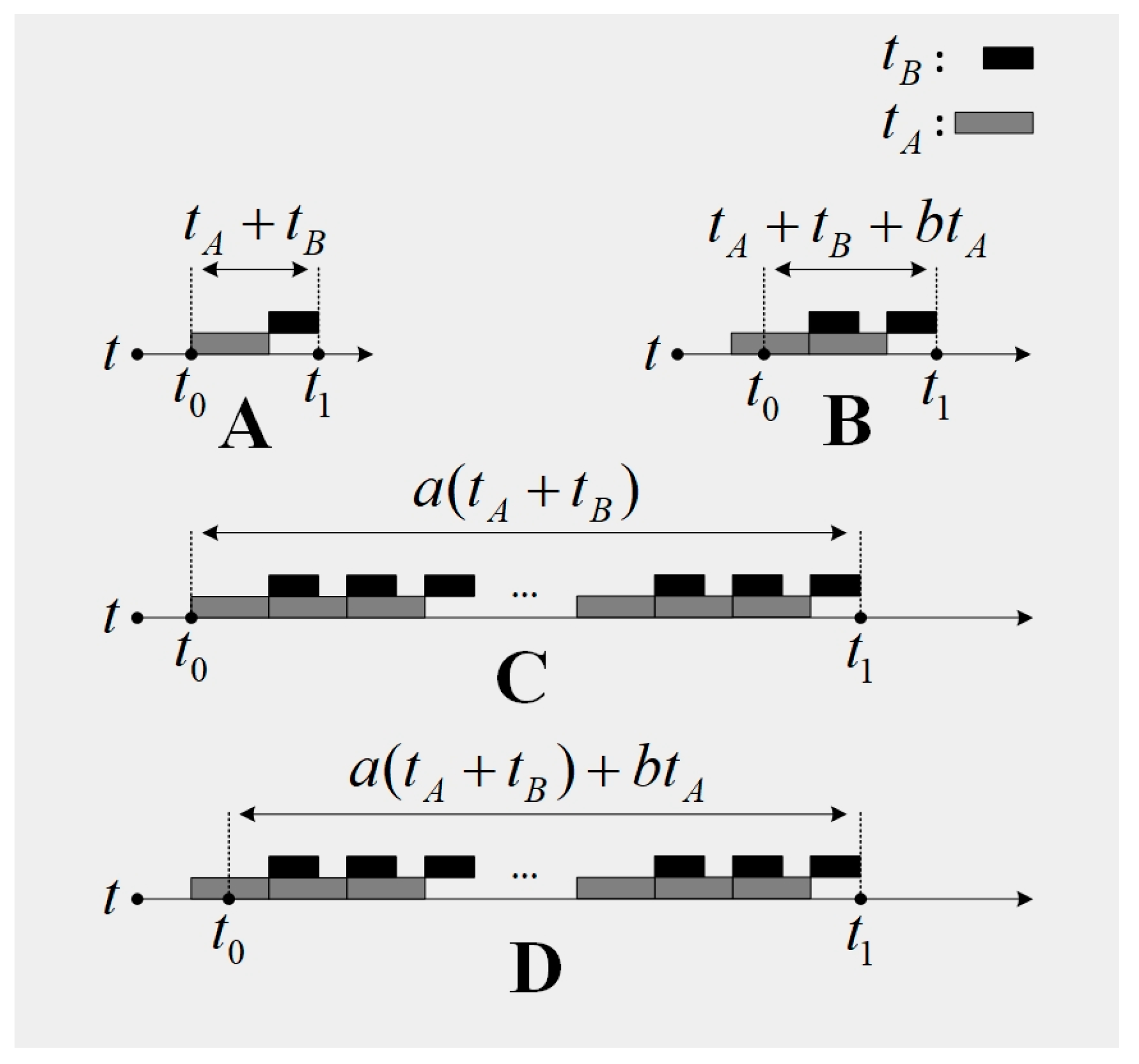
When a diagnostic software is in service, the time lag
can be represented as
, where
,
.
is the time when the fault occurs, and
is the response time of the fault diagnostic software. In our approach,
denotes the number of loops. A loop is a diagnostic procedure which is composed of the signal acquisition and the diagnostic algorithm execution. Due to the low robustness of the diagnostic software, the software should respond to the fault when there is severe interference or some sort of fault in the fault diagnostic software. If this situation takes place, the quantity
may not be 1 (as is described in
Figure 1C,D). Generally, the diagnostic software in time-critical applications is assumed to have enough robustness, therefore the quantity
is set to be
in our approach (as is described in
Figure 1A,B). The quantity
describes the point when the fault occurs in
. Its contribution is to guarantee that the assumption that the diagnostic software in time-critical applications has enough robustness is valid. When
, the fault information in the current collected signal may not be sufficient for a diagnostic procedure to form a response. If the software responds in the current diagnostic procedure, it means that the robustness of the software is too low, which is inconsistent with the assumption that the diagnostic software in time-critical applications has enough robustness. For this reason, the fault diagnostic system should respond in the next diagnostic procedure (as is shown in
Figure 1B). Based on the analysis above, the time lag
can be estimated by
, where
.
3. Materials and Methods
The method adopted in this study involves the following steps: Building the optimization design model, narrowing the solution space through prior knowledge, and solving the model.
3.1. Building the Optimization Design Model
In the parametric design, a fault diagnostic software is often defined as a tuple
, where
is the required accuracy of the designed fault diagnostic software. The required accuracy
is often given in the design document. The diagnostic algorithm
is restricted to the classification method in machine learning. The specific type of the classification method should be determined based on the dataset and the premise of the classification method. The determination of the sampling rate
belongs to the work of the sensor selection before the parametric design. Therefore, the goal of designing the optimal quick diagnostic software can be defined as:
In the context of machine learning, the diagnostic algorithm is a classifier which maps the signal (or time series) to the system state . It is learned by a learning algorithm from a dataset . The dataset consists of many signal samples , and the system state of each sample is known. According to this definition, the diagnostic algorithm should be represented as . Subsequently, the classifier is used to classify the new signal sample in order to diagnose faults.
To guarantee the accuracy of the designed diagnostic software to be no less than the required accuracy
with the consideration of the effect caused by the design objective, the constraint is built into Equation (3). The accuracy of the designed diagnostic software
is estimated by the strategy of model selection in machine learning. At present, there are mainly three methods to estimate the accuracy: Holdout, cross validation, and bootstrapping [
29]. The design method adopts the holdout approach in this paper. This method sets aside part of the dataset
for learning, and this part is called the training set. The remaining part of the dataset
is called the test set. It is used to provide an unbiased evaluation of the accuracy
, as expressed in Equation (2).
in Equation (2) is the number of signal samples in the test set. In general, the holdout method randomly splits the dataset
into the training set and the test set according to a specified proportion, and the common proportions of the training set and the test set are 8:2 or 7:3.
Combining Equations (1) and (3), the problem in the design of the optimal quick diagnostic system can be formulated as Equation (4). It minimizes the response time
and ensures that the accuracy of the designed diagnostic software
is no less than
through finding the optimal parameter
. In Equation (4), the parameters
and
are positive numbers, and the time complexity
is a monotonically increasing function no matter which type of algorithm is employed. Therefore, the objective function is also a monotonically increasing function, and it is equivalent to find the minimal
. Based on this, the optimization model can be equivalently expressed as Equation (5).
3.2. Narrowing the Solution Space Using a Priori Knowledge
The set of natural numbers
is a huge range for solving Equation 5. To improve the efficiency of the procedure, the solution space is narrowed with the help of a priori knowledge about the sampling number
. The sampling number
determines the size of the collected signal. The larger the size of the collected signal, the more information that is available for the diagnostic algorithm. At present, the sampling numbers are 1024, 2048, and 4096 for the signal processing method, which are successfully used for fault diagnosis. Consequently, methods in machine learning also apply these sampling numbers to diagnose and achieve high accuracy [
30,
31,
32]. Obviously, signals of these sizes provide enough information to acquire a satisfactory level of accuracy. Therefore, all these research works actually provide a rational upper bound
for the sampling number, if the required accuracy
is lower than the accuracy related to the upper bound
. On this basis, an optimal parameter
was determined to be in a new smaller range of sampling numbers. Thus, the objective changed from designing a global optimal quick diagnostic system into designing a local one without any design specification violations, as expressed by Equation (6).
3.3. Solving the Model
Theoretically, a signal of the length
is defined as
. The timestamp
is actually a relative time point, and it can generally be ignored. Equation (6) aims to determine a diagnostic method
which applies the shortest possible prefix of the signal
, denoted by
, to reach the required accuracy
. To achieve the goal, an improved wrapper method is proposed. This method is based on the wrapper method, one of the three feature selection methods (filter [
33,
34], wrapper [
33,
35], and embedding [
33,
36]). The wrapper method has three basic steps [
33,
37,
38], which are detailed as follows.
(1) A generation procedure to generate the candidate subset of features: The timestamp is called the feature of a signal, and the value is called the feature value. This step generates a subset of features . The number of elements in is denoted by , which is less than . Then, beside the feature values related to the subset of features , all the other feature values of each sample in the dataset are removed to generate a new dataset .
(2) An evaluation procedure to evaluate the subset: The classifier is learned based on the new dataset . The accuracy of the classifier is estimated, which is denoted by .
(3) A judgment procedure to judge the stopping criterion: Steps 1 and 2 are repeated until the maximal is acquired.
In order to solve the optimization problem in this paper, the wrapper method is improved, which is called Algorithm 1. Upon increasing of the sampling number from 1 to , the subset of features is generated through the extraction of the first elements in the feature set in the generation procedure. In the evaluation procedure, the holdout method is applied to evaluate the accuracy of the classifier . The stopping criterion is that the accuracy must be no less than the required accuracy . When the criterion is met, the optimal sampling number is obtained. The tuple is determined, thus the design is completed. As mentioned previously, the precondition that the required design accuracy be lower than the accuracy related to the upper bound should be satisfied. If not, the solution may not be obtained.
| Algorithm 1 Algorithm of the optimal solution |
| Step 1. Determine the dataset , the classifier , the learning algorithm , the required accuracy , the proportion in the holdout method. |
| Step 2. Initialize , = 0, ; |
| Step 3. Execute the iteration below: |
| While : |
| If : |
| ; |
| For every sample in : |
| take into |
| End |
| Learn the classifier using the learning algorithm on the dataset ; |
| Estimate using the holdout method; |
| |
| Else: |
| End while |
| Step 4. Output the optimal sampling number |
6. Conclusions
This study proposed a parametric design method for an optimal quick diagnostic system. Using this method, an optimal quick diagnostic system can be obtained, which has the smallest response time and a pre-defined accuracy. By means of experimental verification, the feasibility of the parametric design method was validated. Contrary to other existing methods, the proposed approach fulfills the following three characteristics:
First, the measure of the response time was proposed in this method, which provides a common standard to quantitatively assess the improvement of the response time.
Secondly, using the parametric design method proposed in this paper, the designed fault diagnostic software exhibited an obvious improvement in the response time to faults as compared with the response times of traditional methods with the same vibration data.
Thirdly, the parametric design method exhibited superiority in the trade-off between the accuracy and the response time.
Additionally, the experimental results revealed that the higher the required accuracy is, the less robust the designed diagnostic software is to noise and uncertainty. At the same time, the experimental results demonstrate that serious faults are guaranteed to be diagnosed more quickly by the diagnostic software; although, the more serious the fault is, the more easily the feature will be recognized.


