A Knowledge-Driven Approach for 3D High Temporal-Spatial Measurement of an Arbitrary Contouring Error of CNC Machine Tools Using Monocular Vision


Abstract
1. Introduction
2. Principle for Contouring Error Detection Using a Single Camera
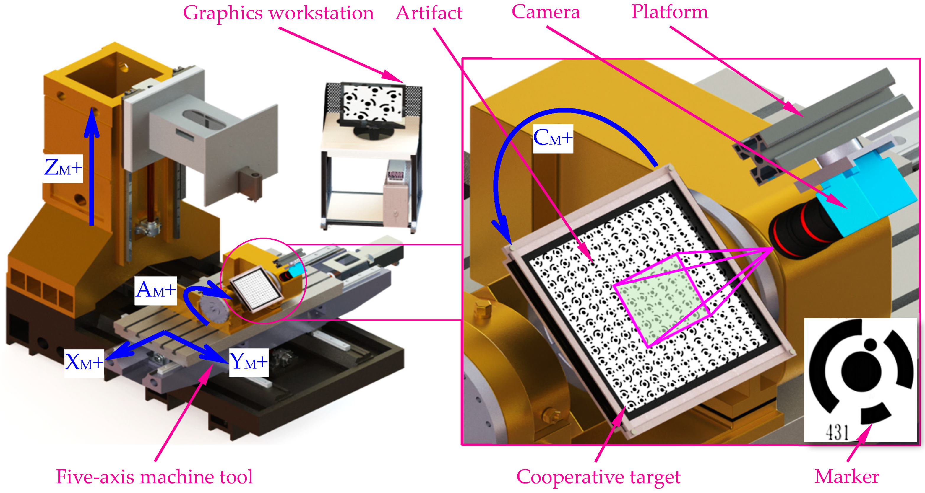
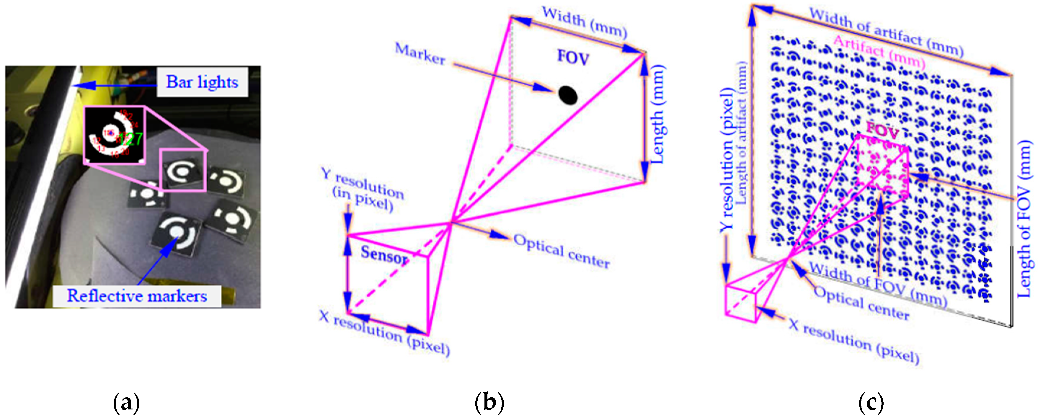
2.1. Measurement System and Principle
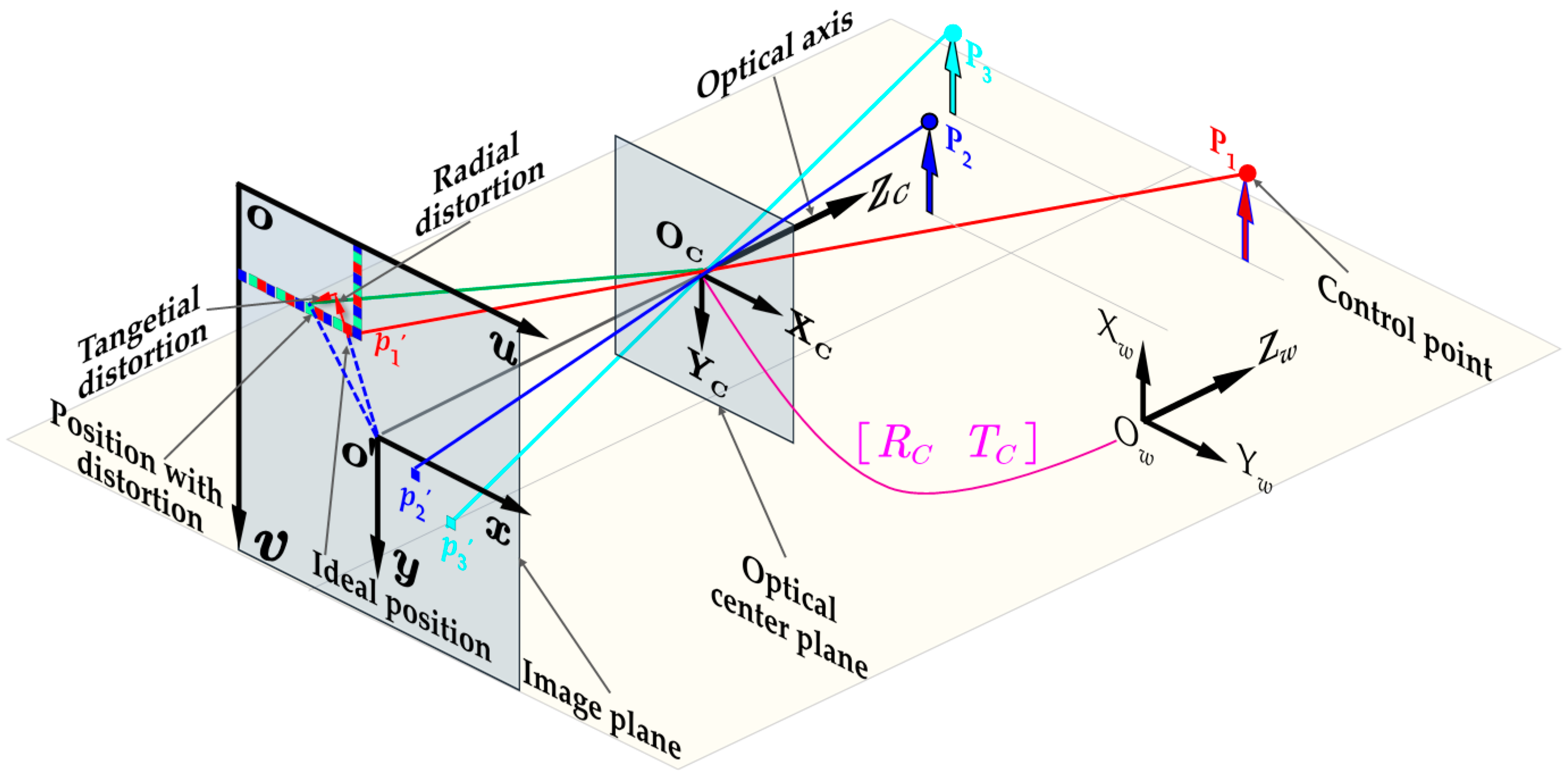
2.2. Camera Calibration Method Considering the Distortion Partition of DOF
3. High Precision 3D Positioning of Machine Tool Movement
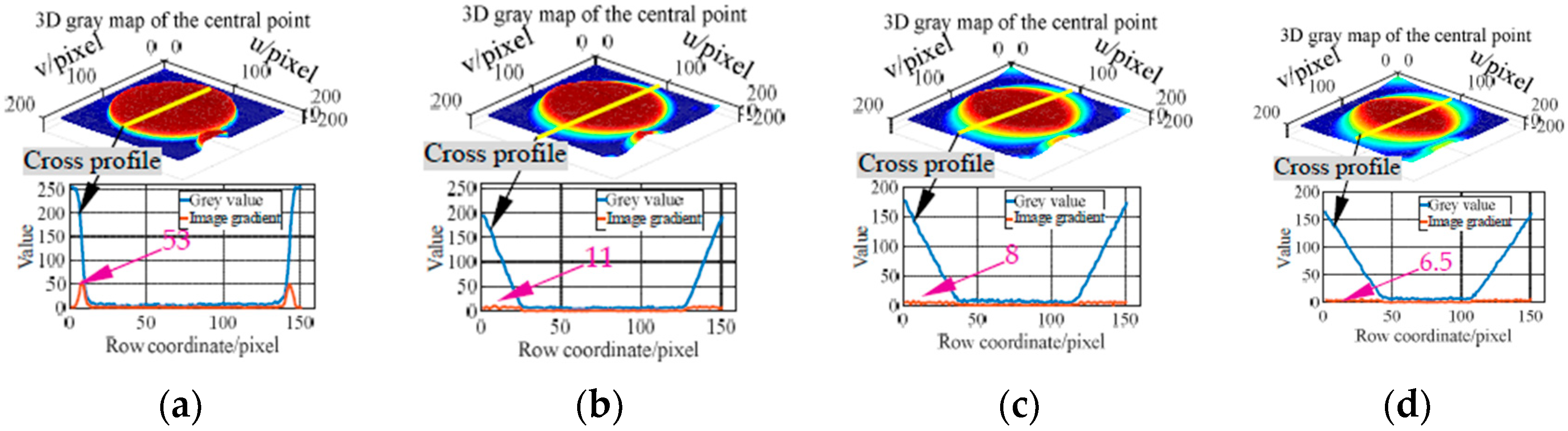
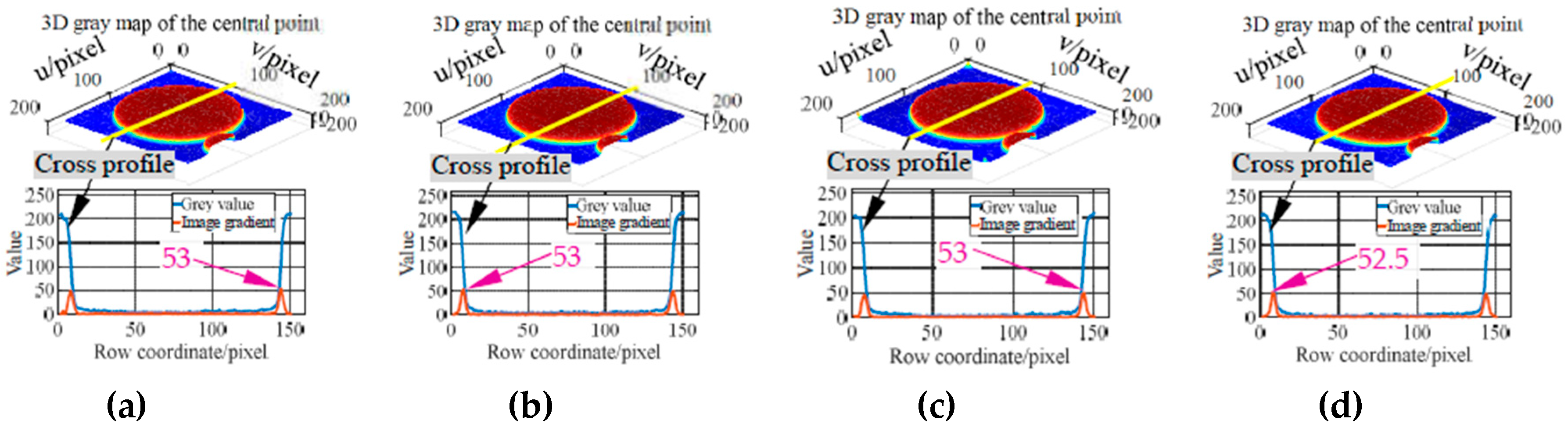
3.1. High-Quality Image Acquisition for Machine Tool Movement
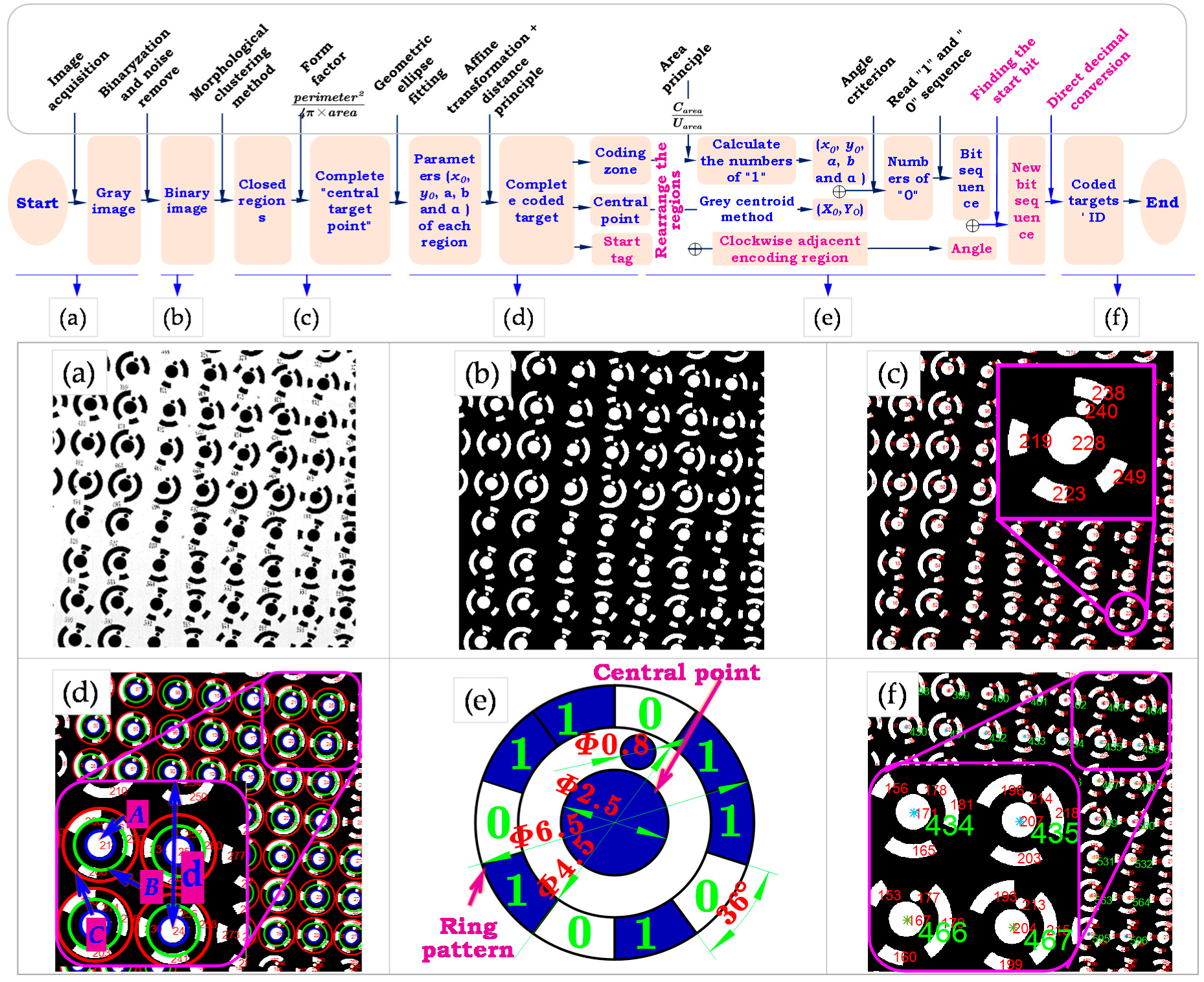
3.2. Accurate Encoding and Identification Method for Coded Targets
- A)
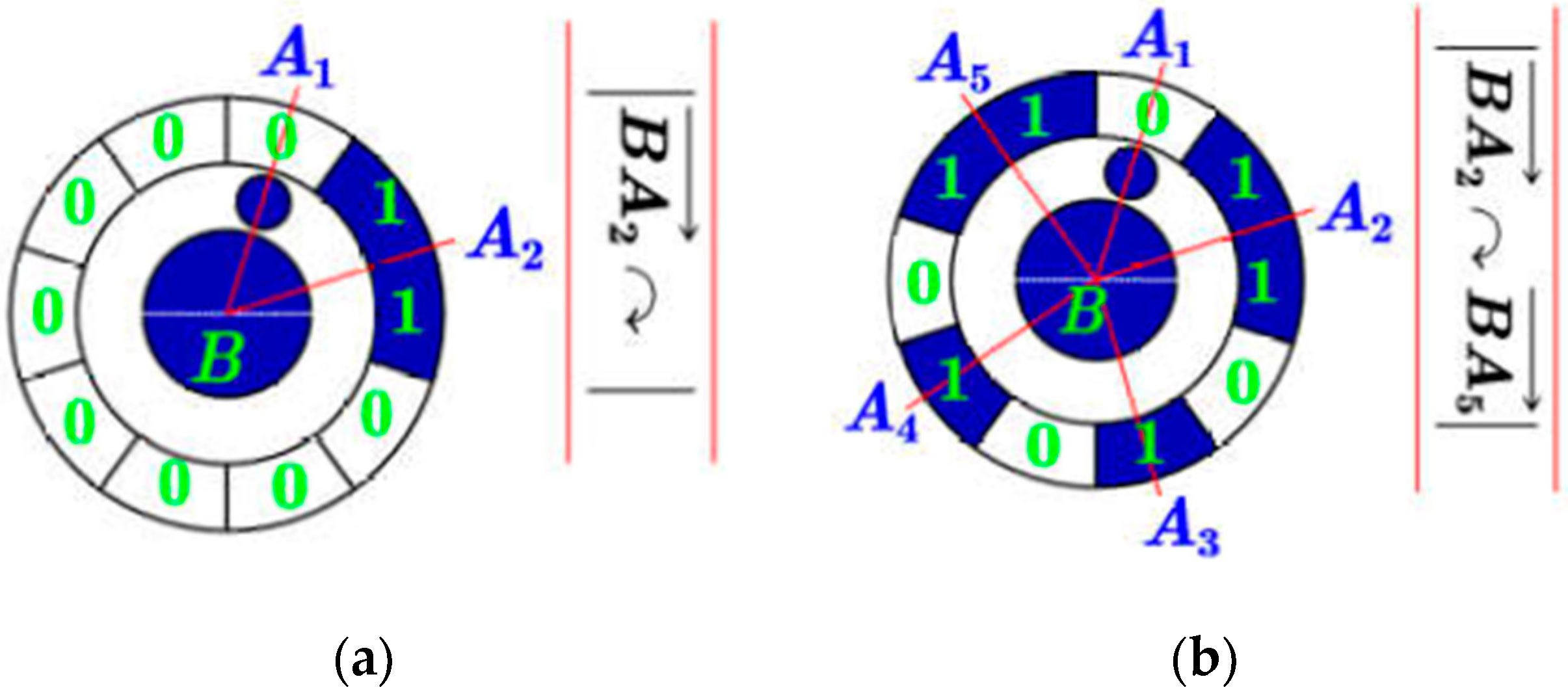
- Case 1: only one encoding region around the central pointAs shown in Figure 10a, suppose that this encoding region consists of “1”, then the number of “0” with respect to the non-encoding region is , and we get the binary sequence .
- B)
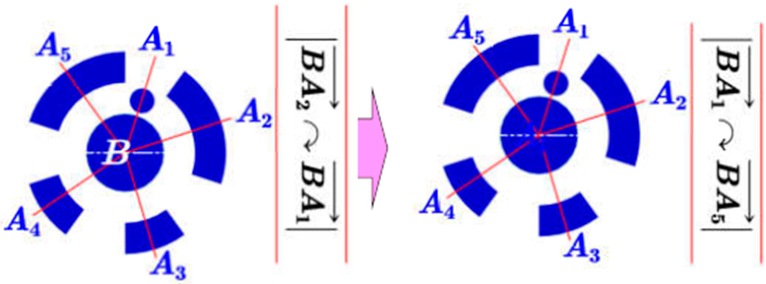
- Case 2: more than one encoding region around the central pointThe numbers of “0” in the non-encoding region between two adjacent encoding regions (Figure 10b) can be deduced by . Where describes the angle formed by adjacent two vectors (e.g., ), ; and are the numbers of “1” in two adjacent encoding regions. By traversing the entire ring pattern, we get the binary sequence of..
- A)
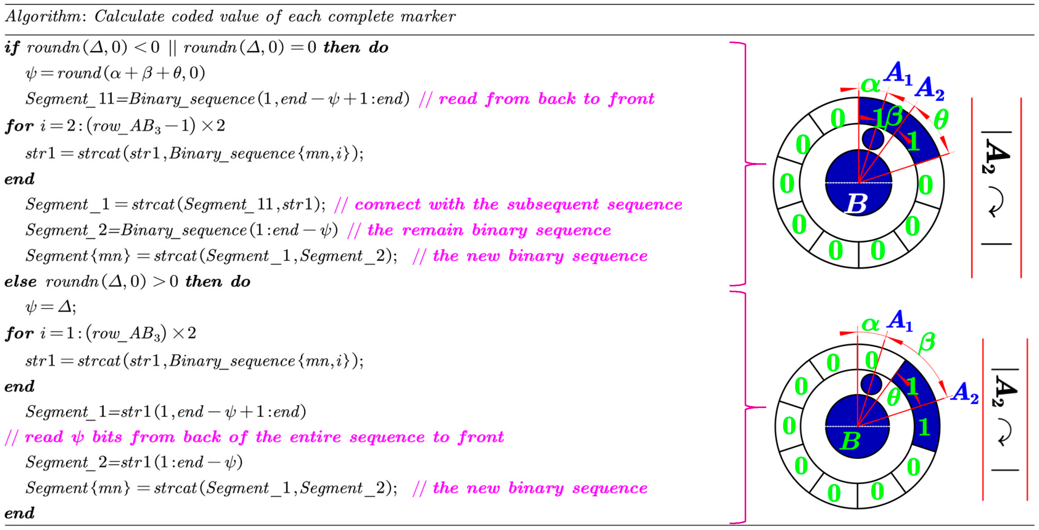
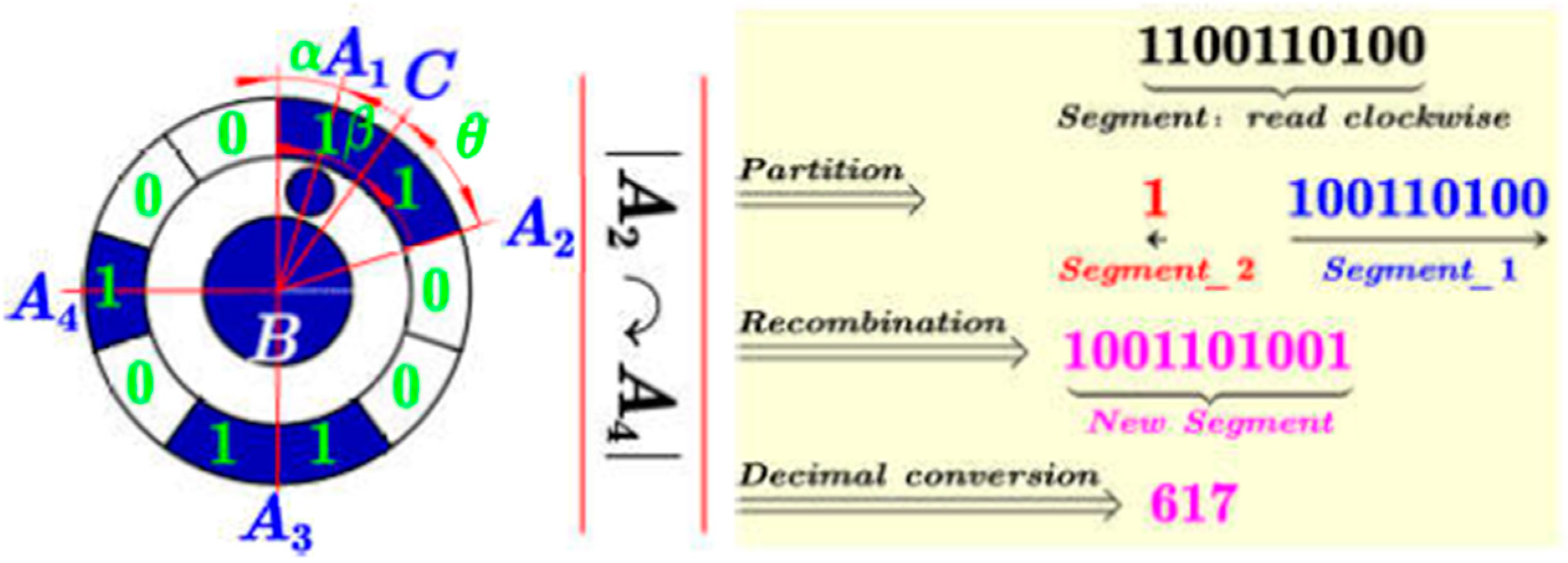
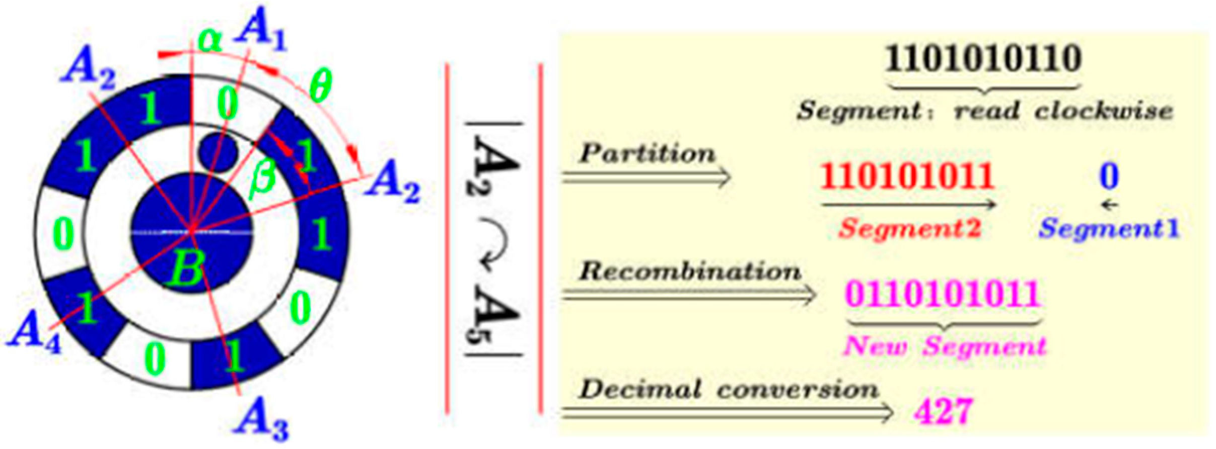
- Case 1: if orAs shown in Figure 12, Let , and assume the first encoding region consists of number of “1”, where . First, numbers of “1” from the back to the front of this sequence are read and then connected with the following sequence to get the ; while the remain number of “1” in the first encoding region is denoted by . Finally, the new segment is obtained by connecting to .
- B)
- Case 2:binary numbers from the back of the entire binary sequence to the front are read to form (Figure 13), and the remain binary sequence is denoted by . Then, the new segment is obtained by connecting to .
4. 3D High Spatial-Temporal Measurement of Large-Scale and Relatively High-Dynamic Contouring Error
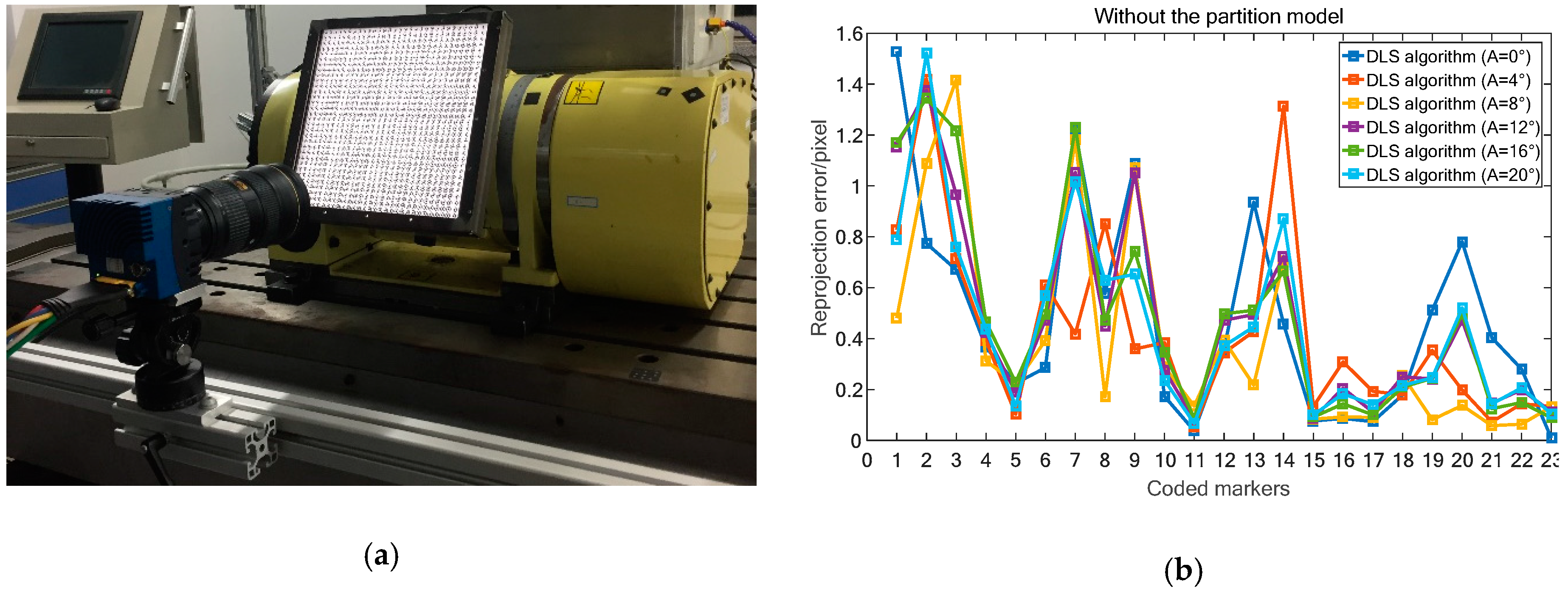
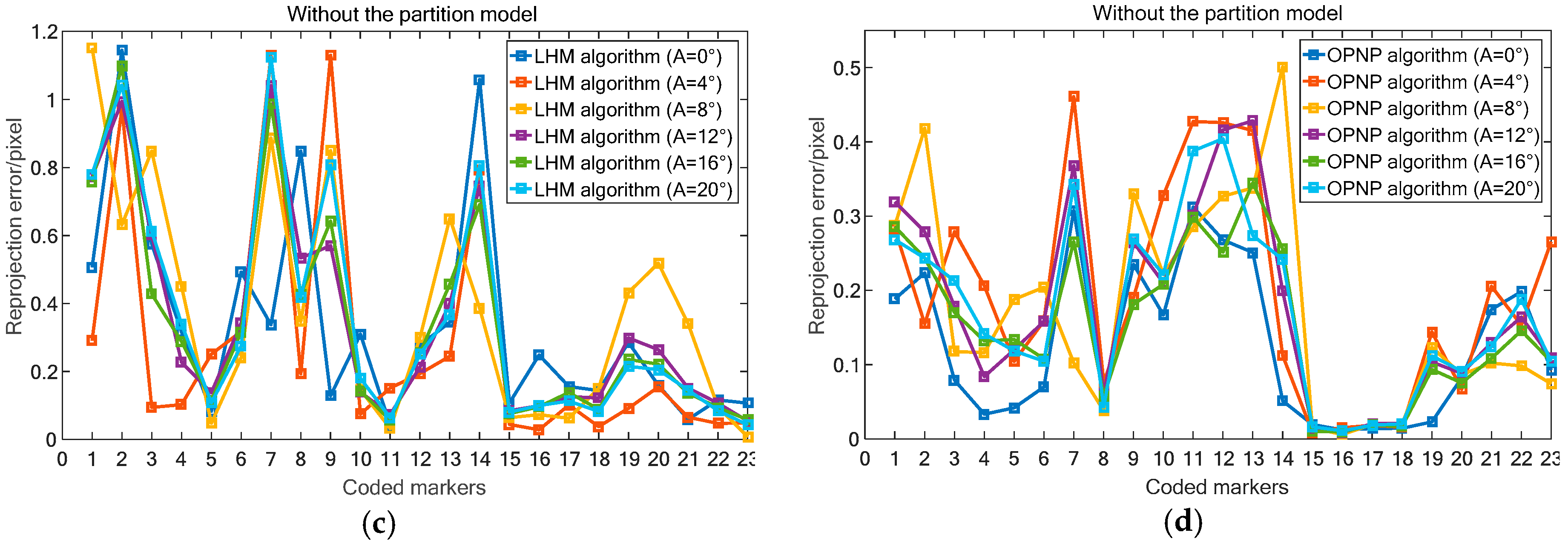
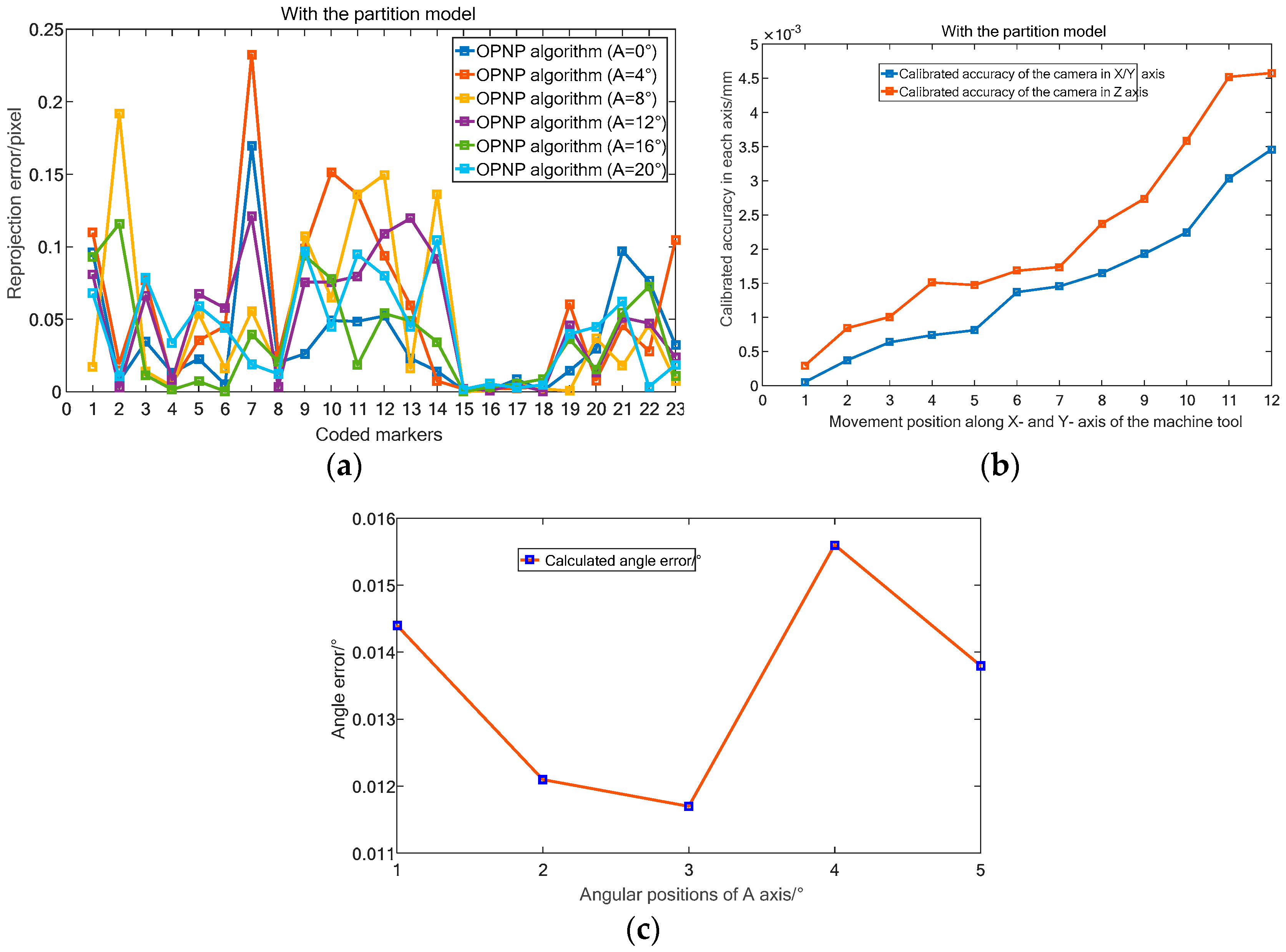
4.1. Pose Estimation Algorithms Comparison
4.2. Wide Range Contouring Error Detection
5. Contouring Error Detection Test and Vision Measurement Accuracy Verification
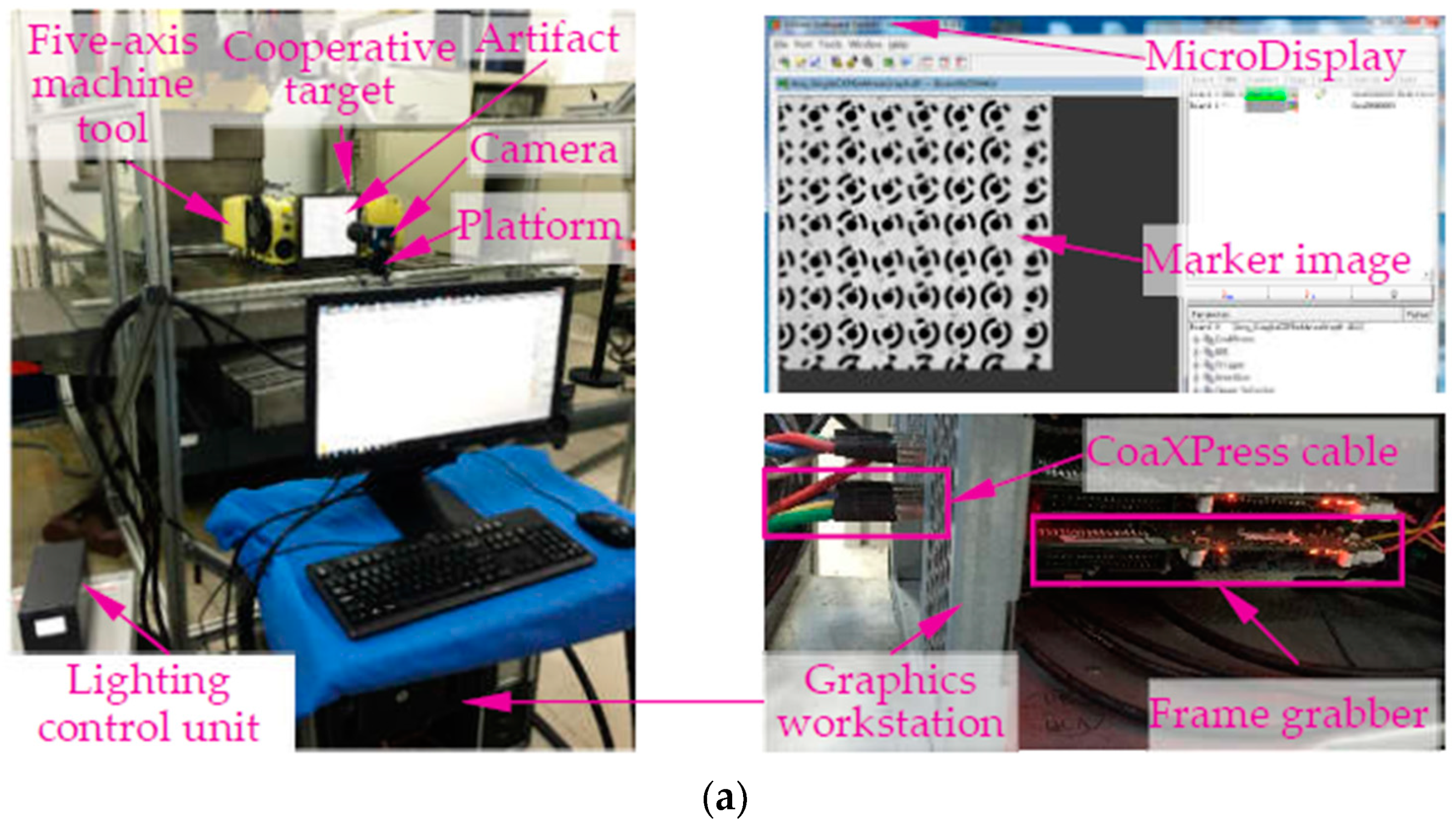
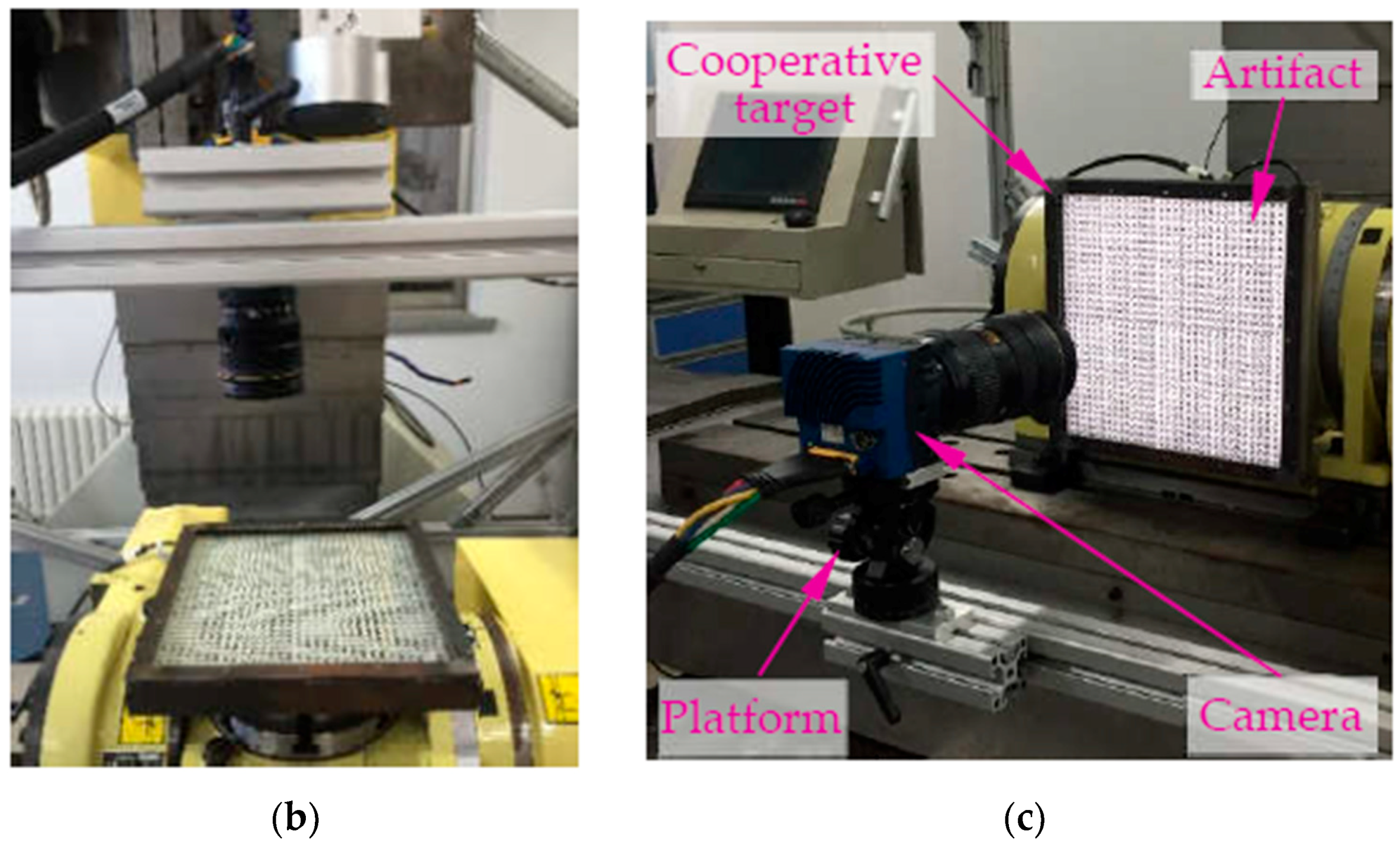
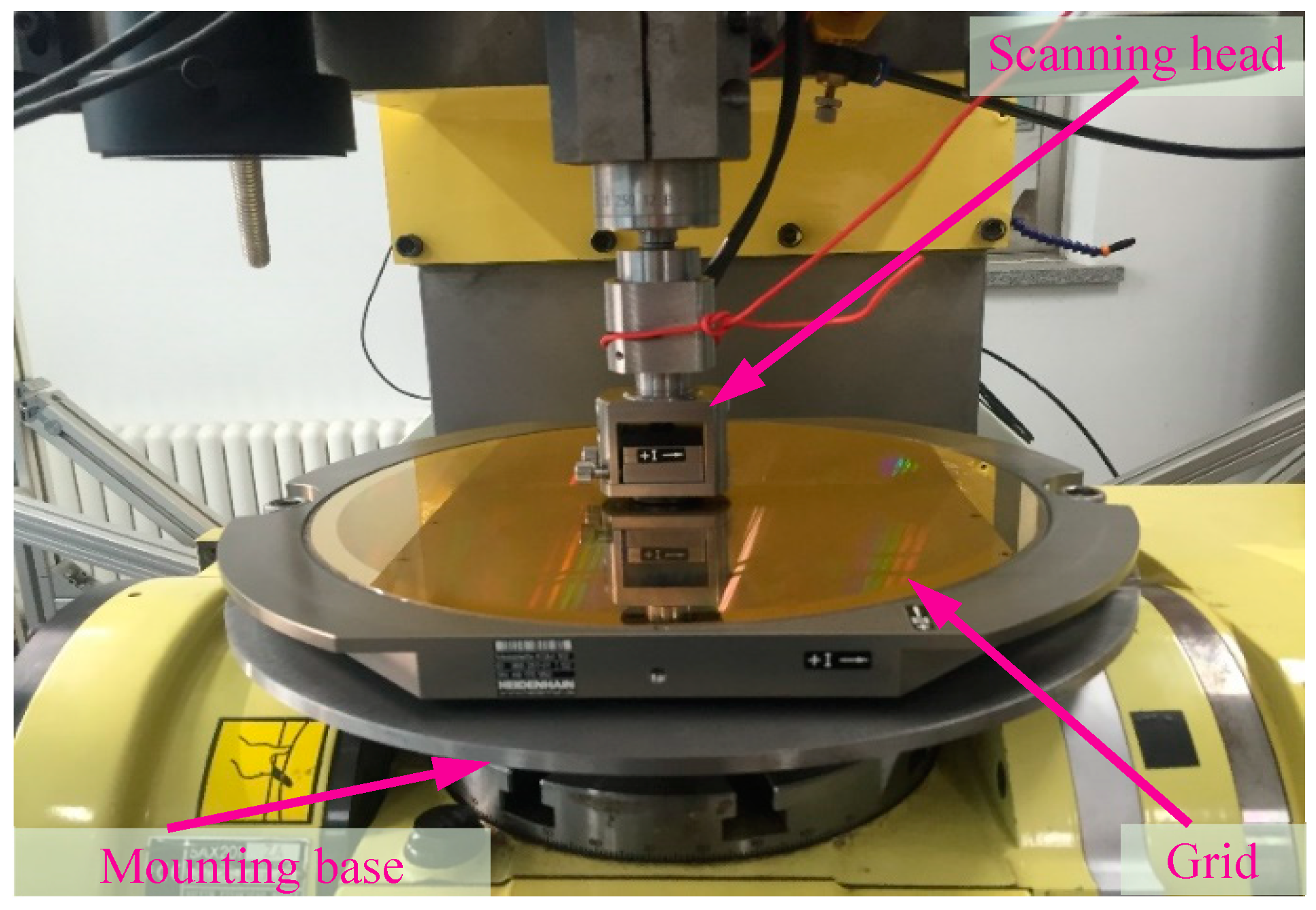
5.1. Experimental Equipment and Tested Trajectories
5.2. Experiment for Verifying the Proposed Calibration Method
- (1)
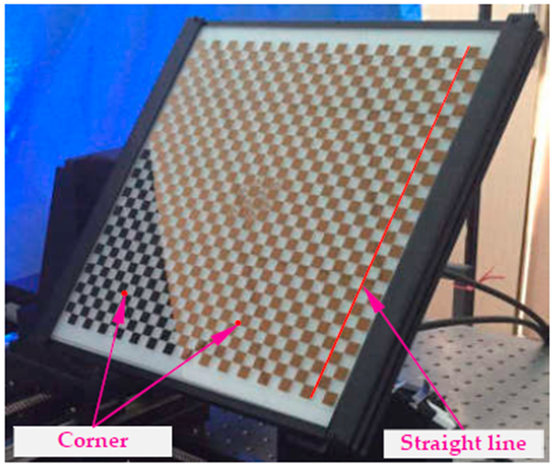
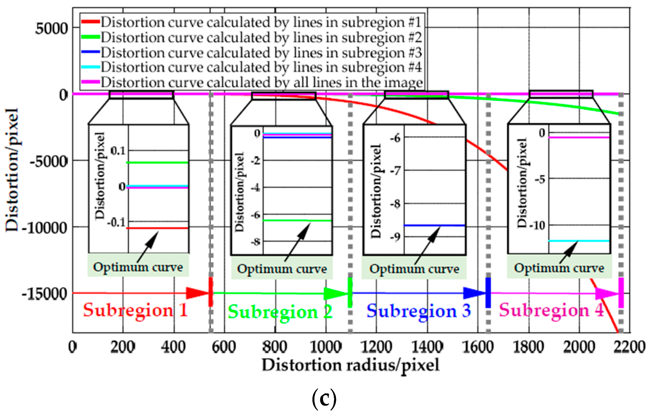
- Accuracy verification of equal-radius partition modelAs shown in Figure 21b,c, distortion curve of each subregion is different from that of calculated by all the lines in the image. Firstly, the performance of in-plane distortion partition model is judged by the straightness error after distortion correction. As illustrated in Table 3, the maximum and average straightness errors of each subregion are smaller than that are calculated by all the lines in the image, which indicate the accuracy of the proposed partition method. The optimal distortion curve for each subregion can be seen in the enlarged view of Figure 21c.
- (2)
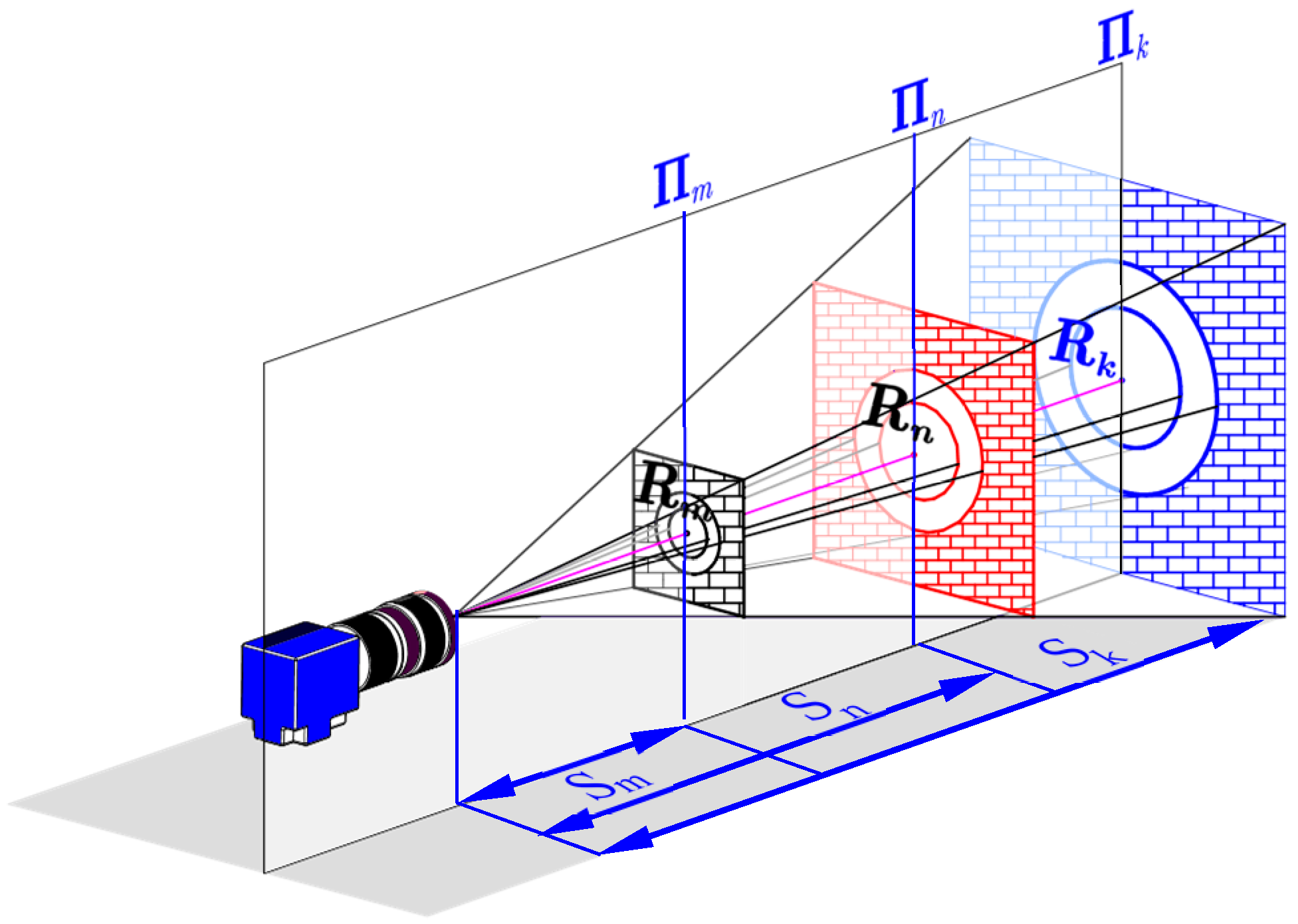
- Accuracy verification of the 3D distortion partition modelThen, based on the front and rear object planes with known depths and the calibrated distortion parameters, the distortion coefficients on each partition of the two middle object planes are estimated by the method in Section 2.2. Thereafter, the derived distortions of the two middle planes are compared with that calculated directly by the plumb-line method to verify the accuracy of the proposed DOF distortion partition model.Table 4 illustrates the difference |C − O| between the distortion calculated with or without DOF distortion partition model and the observed one. The results indicate that the maximum and average differences are 1.75 μm and 0.86 μm, while the distortion differences calculated without the partition model are more than twice the corresponding difference calculated with the partition distortion, which show the high accuracy of the proposed partition method.
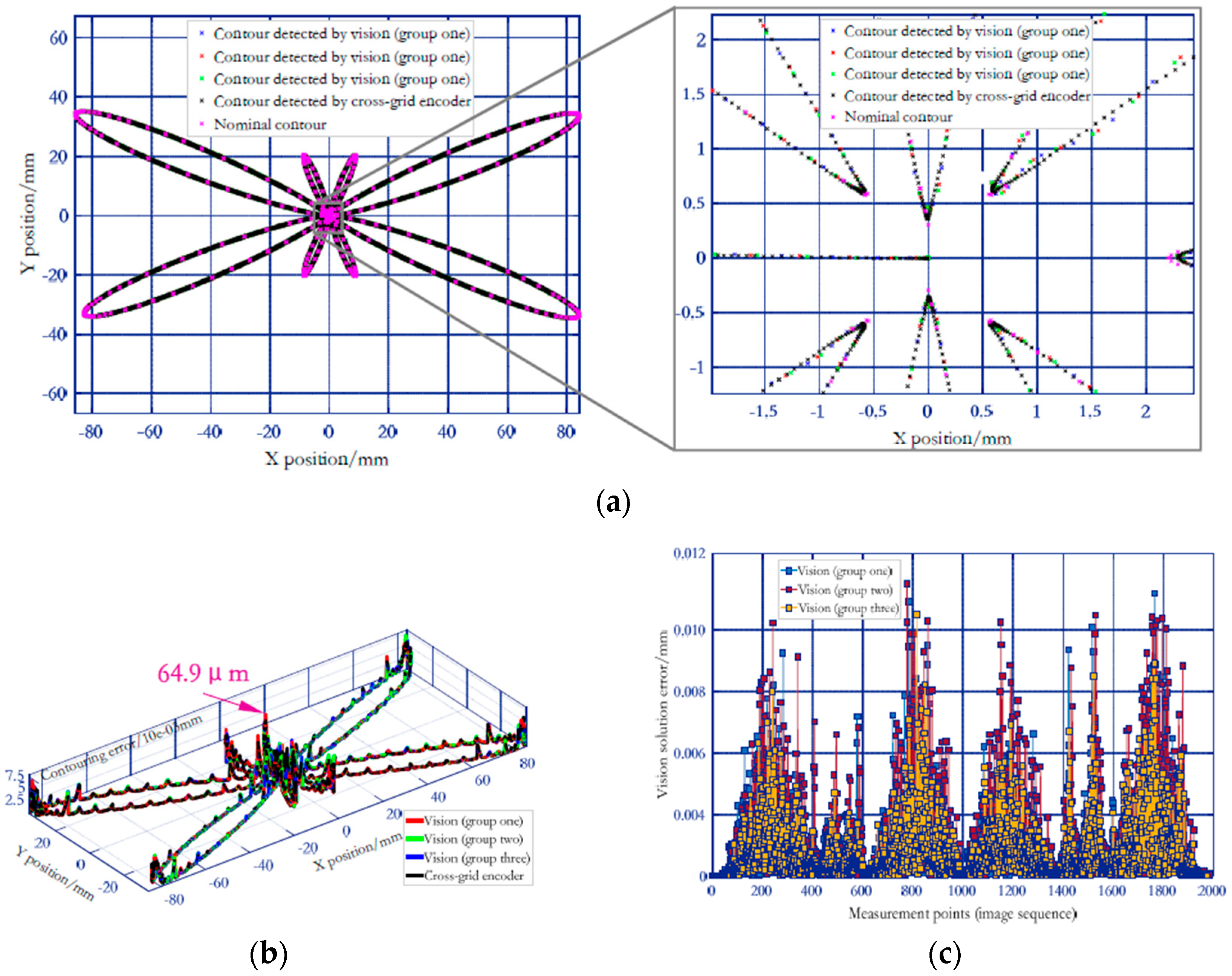
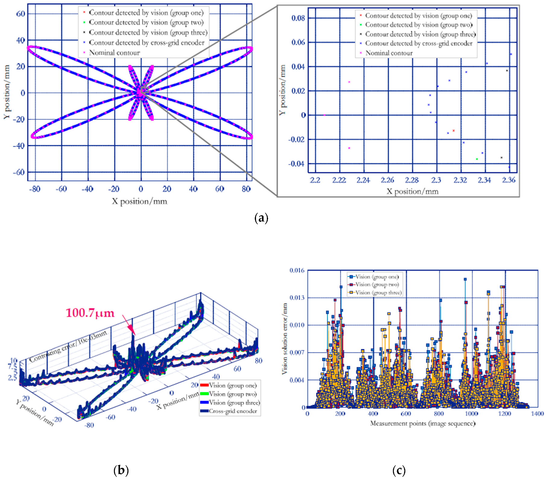
5.3. Case Study for Illustrating Advantages in 3D High Temporal-Spatial Measurement
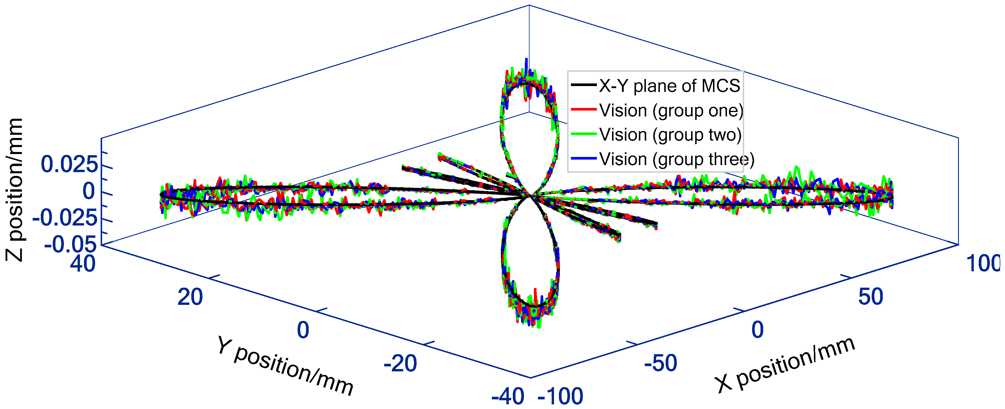
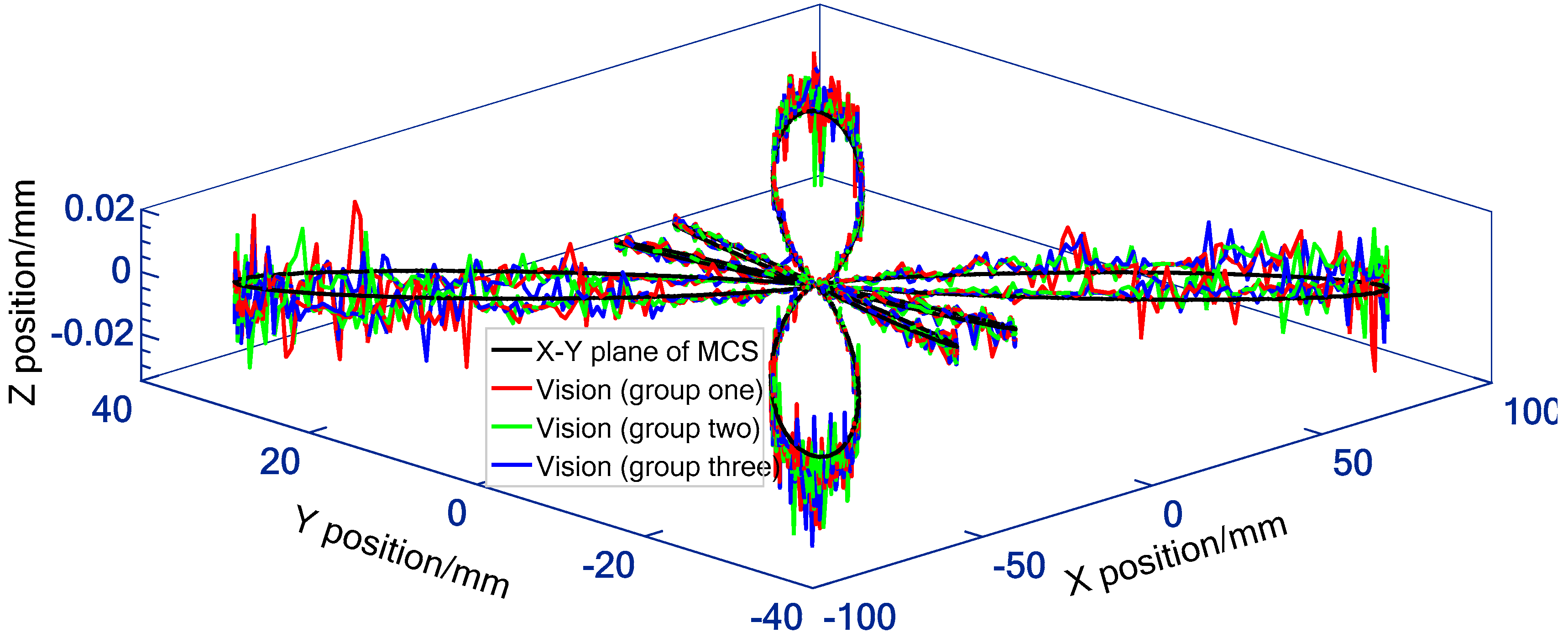
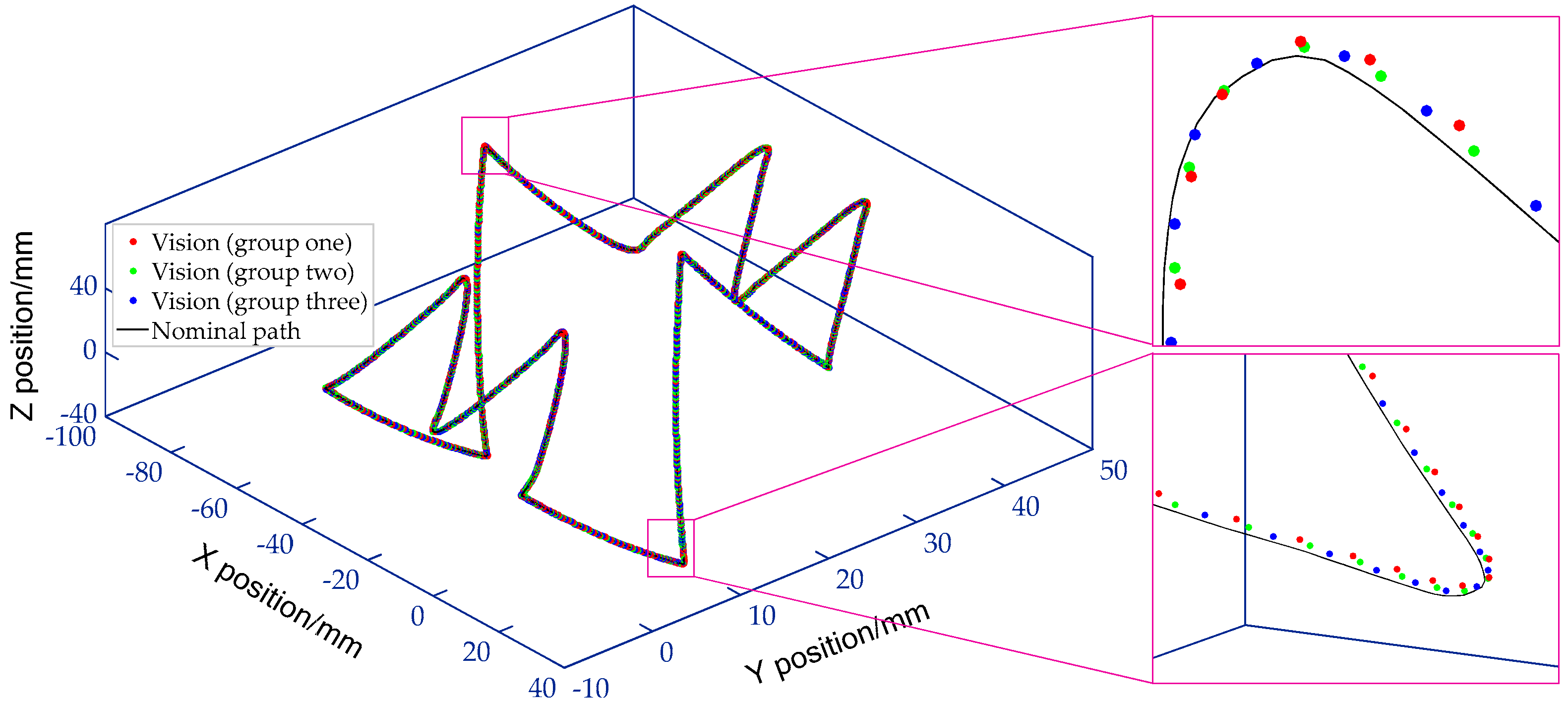
5.4. Case Study for Highlighting 3D Detection of Contouring Error of a Space Trajectory
5.5. Remarks on Major Contributors for Measurement Uncertainties
6. Conclusions
Supplementary Materials
Author Contributions
Funding
Conflicts of Interest
References
- Smith, G.T. Machine Tool Metrology: An Industrial Handbook, 1st ed.; Springer Nature: Cham, Switzerland, 2016; pp. 345–380. ISBN 978-3-319-25109-7. [Google Scholar]
- ISO 230 Series. Test Code for Machine Tools; An International Standard by the International Standard Organization; International Standard Organization: Genève, Switzerland.
- ISO 13041 Series. Test Conditions for Numerically Controlled Turning Machines and Turning Centres; An International Standard by the International Standard Organization; International Standard Organization: Genève, Switzerland.
- ISO 10360 Series. Geometrical Product Specifications (GPS)–Acceptance and Reverification Tests for Coordinate Measuring Machines (CMM); An International Standard by the International Standard Organization; International Standard Organization: Genève, Switzerland.
- ISO/TR 230-11:2018 (E). Test Code for Machine Tools, Part 11: Measuring Instruments Suitable for Machine Tool Geometry Tests; An International Standard by the International Standard Organization; International Standard Organization: Genève, Switzerland, 2018. [Google Scholar]
- Chen, J.; Lin, S.; He, B. Geometric error measurement and identification for rotary table of multi-axis machine tool using double ballbar. Int. J. Mach. Tools Manuf. 2014, 77, 47–55. [Google Scholar] [CrossRef]
- Lee, K.I.; Yang, S.H. Measurement and verification of position-independent geometric errors of a five-axis machine tool using a double ball-bar. Int. J. Mach. Tools Manuf. 2013, 70, 45–52. [Google Scholar] [CrossRef]
- Du, Z.; Zhang, S.; Hong, M. Development of a multi-step measuring method for motion accuracy of NC machine tools based on cross grid encoder. Int. J. Mach. Tools Manuf. 2010, 50, 270–280. [Google Scholar] [CrossRef]
- Otsuki, T.; Sasahara, H.; Sato, R. A method for the evaluation and magnified representation of two-dimensional contouring error. Precis. Eng. 2017, 50, 433–439. [Google Scholar] [CrossRef]
- Brecher, C.; Behrens, J.; Klatte, M.; Lee, T.; Tzanetos, F. Measurement and analysis of thermo-elastic deviation of five-axis machine tool using dynamic R-test. Procedia CIRP 2018, 77, 521–524. [Google Scholar] [CrossRef]
- Zhong, L.; Bi, Q.; Huang, N.; Wang, Y. Dynamic accuracy evaluation for five-axis machine tools using S trajectory deviation based on R-test measurement. Int. J. Mach. Tools Manuf. 2018, 125, 20–33. [Google Scholar] [CrossRef]
- Lee, H.H.; Son, J.G.; Yang, S.H. Techniques for measuring and compensating for servo mismatch in machine tools using a laser tracker. Int. J. Adv. Manuf. Technol. 2017, 92, 2919–2928. [Google Scholar] [CrossRef]
- Aguado, S.; Santolaria, J.; Samper, D.; Aguilar, J.J. Forecasting method in multilateration accuracy based on laser tracker measurement. Meas. Sci. Technol. 2017, 28, 25011. [Google Scholar] [CrossRef]
- Ibaraki, S.; Tanizawa, Y. Vision-based measurement of two-dimensional positioning errors of machine tools. J. Adv. Mech. Des. Syst. Manuf. 2011, 5, 315–328. [Google Scholar] [CrossRef]
- Liu, W.; Li, X.; Jia, Z.; Yan, H.; Ma, X. A three-dimensional triangular vision-based contouring error detection system and method for machine tools. Precis. Eng. 2017, 50, 85–98. [Google Scholar] [CrossRef]
- Liu, W.; Li, X.; Jia, Z.; Li, H.; Ma, X.; Yan, H.; Ma, J. Binocular-vision-based error detection system and identification method for PIGEs of rotary axis in five-axis machine tool. Precis. Eng. 2018, 51, 208–222. [Google Scholar] [CrossRef]
- Bryan, J.B. A simple method for testing measuring machines and machine tools Part 1: Principles and applications. Precis. Eng. 1982, 4, 61–69. [Google Scholar] [CrossRef]
- Bryan, J.B. A simple method for testing measuring machines and machine tools. Part 2: Construction details. Precis. Eng. 1982, 4, 125–138. [Google Scholar] [CrossRef]
- ISO 10791-6:2014 (E). Test Conditions for Machining Centers, Part 6: Accuracy of Speeds and Interpolations; An International Standard by International Standard Organization; International Standard Organization: Genève, Switzerland, 2014. [Google Scholar]
- ISO 230-4:2005. Test Code for Machine Tools, Part 4: Circular Tests for Numerically Controlled Machine Tools; An International Standard by International Standard Organization; International Standard Organization: Genève, Switzerland, 2005. [Google Scholar]
- ASME B5.54-2005. Methods for Performance Evaluation of Computer Numerically Controlled Machining Centers; An American National Standard; ASME International: New York, NY, USA, 2005. [Google Scholar]
- Lee, K.I.; Lee, D.M.; Yang, S.H. Parametric modeling and estimation of geometric errors for a rotary axis using double ball-bar. Int. J. Mach. Tools Manuf. 2018, 62, 741–750. [Google Scholar] [CrossRef]
- Jiang, X.; Cripps, R.J. A method of testing position independent geometric errors in rotary axes of a five-axis machine tool using a double ball bar. Int. J. Mach. Tools Manuf. 2015, 89, 151–158. [Google Scholar] [CrossRef]
- Weikert, S. R-test, a new device for accuracy measurements on five axis machine tools. CIRP Ann-Manuf. Technol. 2004, 53, 429–432. [Google Scholar] [CrossRef]
- Bringmann, B.; Knapp, W. Model-based ‘chase-the-ball’ calibration of a 5-axes machining center. CIRP Ann-Manuf. Technol. 2006, 55, 531–534. [Google Scholar] [CrossRef]
- Hong, C.; Ibaraki, S. Non-contact R-test with laser displacement sensors for error calibration of five-axis machine tools. Precis. Eng. 2013, 37, 159–171. [Google Scholar] [CrossRef]
- Zargarbashi, S.H.H.; Mayer, J.R.R. Single setup estimation of a five-axis machine tool eight link errors by programmed end point constraint and on the fly measurement with Capball sensor. Int. J. Mach. Tools Manuf. 2009, 49, 759–766. [Google Scholar] [CrossRef]
- Ibaraki, S.; Kakino, Y.; Lee, K.; Ihara, Y.; Braasch, J.; Eberherr, A. Diagnosis and compensation of motion errors in NC machine tools by arbitrary shape contouring error measurement. Laser. Metrol. Mach. Perform. 2001, 38, 59–68. [Google Scholar]
- Lau, K.; Hocken, R.J.; Haight, W.C. Automatic laser tracking interferometer system for robot metrology. Precis. Eng. 1986, 8, 3–8. [Google Scholar] [CrossRef]
- Hughes, E.B.; Wilson, A.; Peggs, G.N. Design of a high-accuracy CMM based on multi-lateration techniques. CIRP Ann-Manuf. Technol. 2000, 49, 391–394. [Google Scholar] [CrossRef]
- Muralikrishnan, B.; Phillips, S.; Sawyer, D. Laser trackers for large-scale dimensional metrology: A review. Precis. Eng. 2016, 44, 13–28. [Google Scholar] [CrossRef]
- Zhao, D.; Bi, Y.; Ke, Y. An efficient error compensation method for coordinated CNC five-axis machine tools. Int. J. Mach. Tools Manuf. 2017, 123, 105–115. [Google Scholar] [CrossRef]
- Li, X.; Liu, W.; Pan, Y.; Liang, B.; Zhou, M.; Li, H.; Wang, F.; Jia, Z. Monocular-vision-based contouring error detection and compensation for CNC machine tools. Precis. Eng. 2019, 55, 447–463. [Google Scholar] [CrossRef]
- Sladek, J.; Gaska, A. Evaluation of coordinate measurement uncertainty with use of virtual machine model based on Monte Carlo method. Measurement 2012, 45, 1564–1575. [Google Scholar] [CrossRef]
- Skibicki, J.D.; Judek, S. Influence of vision measurement system spatial configuration on measurement uncertainty, based on the example of electric traction application. Measurement 2018, 116, 281–298. [Google Scholar] [CrossRef]
- Kohut, P.; Holak, K.; Martowicz, A. An uncertainty propagation in developed vision based measurement system aided by numerical and experimental tests. J. Theor. Appl. Mech. 2012, 50, 1049–1061. [Google Scholar]
- Fooladgar, F.; Samavi, S.; Soroushmehr, S.M.R.; Shirani, S. Geometrical analysis of localization error in stereo vision systems. IEEE Sens. J. 2013, 13, 4236–4246. [Google Scholar] [CrossRef]
- Sankowski, W.; Wkodarczyk, M.; Kacperski, D.; Grabowski, K. Estimation of measurement uncertainty in stereo vision system. Image Vis. Comput. 2017, 61, 70–81. [Google Scholar] [CrossRef]
- Aydin, I. A new approach based on firefly algorithm for vision-based railway overhead inspection system. Measurement 2012, 74, 43–55. [Google Scholar] [CrossRef]
- Zhang, Z. A flexible new technique for camera calibration. IEEE Trans. Pattern Anal. Mach. Intell. 2000, 22, 1330–1334. [Google Scholar] [CrossRef]
- Fischler, M.A.; Bolles, R.C. Random sample consensus: a paradigm for model fitting with applications to image analysis and automated cartography. Commun. ACM 1981, 24, 381–395. [Google Scholar] [CrossRef]
- Duane, C.B. Close–range camera calibration. Photogramm. Eng. 1971, 37, 855–866. [Google Scholar]
- Fryer, J.G.; Brown, D.C. Lens distortion for close-range photogrammetry. Photogramm. Eng. Remote Sens. 1986, 52, 51–58. [Google Scholar]
- Sun, P.; Lu, N.; Dong, M. Modelling and calibration of depth-dependent distortion for large depth visual measurement cameras. Opt. Express 2017, 25, 9834–9847. [Google Scholar] [CrossRef] [PubMed]
- Jia, Z.; Ma, X.; Liu, W.; Lu, W.; Li, X.; Chen, L.; Wang, Z.; Cui, X. Pose measurement method and experiments for high-speed rolling targets in a wind tunnel. Sensors 2014, 14, 23933–23953. [Google Scholar] [CrossRef] [PubMed]
- Bergamasco, F.; Albarelli, A.; Rodola, E.; Torsello, A. RUNE-Tag: a high accuracy fiducial marker with strong occlusion resilience. In Proceedings of the 2011 IEEE Conference on Computer Vision and Pattern Recognition, Colorado Springs, CO, USA, 20–25 June 2011. [Google Scholar]
- Peng, H.; Herskovits, E.; Davatzikos, C. Bayesian clustering methods for morphological analysis of MR images. In Proceedings of the 2002 IEEE International Symposium on Biomedical Imaging, Washington, DC, USA, 7–10 July 2002. [Google Scholar]
- Luhmann, T.; Robson, S.; Kyle, S.; Boehm, J. Close-Range Photogrammetry and 3D Imaging, 2nd ed.; De Gruyter: Berlin, Germany, 2013; pp. 223–454. ISBN 978-3-11-030278-3. [Google Scholar]
- Hesch, J.A.; Roumeliotis, S.I. A direct least-squares (DLS) method for PnP. In Proceedings of the 2011 IEEE international conference on computer vision, Barcelona, Spain, 6–13 November 2011. [Google Scholar]
- Lu, C.P.; Hager, G.D.; Mjolsness, E. Fast and globally convergent pose estimation from video images. IEEE Trans. Pattern Anal. Mach. Intell. 2000, 22, 610–622. [Google Scholar] [CrossRef]
- Zheng, Y.; Kuang, Y.; Sugimoto, S.; Astrom, K.; Okutomi, M. Revisiting the PnP problem: A fast, general and optimal solution. In Proceedings of the 2013 IEEE International Conference on Computer Vision, Sydney, Australia, 1–8 December 2013. [Google Scholar]
- Yi, S.; Haralick, R.M.; Shapiro, L.G. Error propagation in machine vision. Mach. Vis. Appl. 1994, 7, 93–114. [Google Scholar] [CrossRef]


| Index | Parameter Values |
|---|---|
| Camera and resolution | Camera: EoSens® 25 CXP; Full resolution: 5120 × 5120 pixels |
| Lens | Nikon 24–70 mm |
| Lens mount | F-Mount |
| Exposure time | 3000 μs |
| Spatial resolution (without subpixel accuracy) | 0.0195 mm/pixel |
| Size of the measurement basis | 231 mm × 231 mm |
| FOV | 60 mm × 60 mm |
| Light source | Flat backlight |
| Light-emitting area | 250 mm × 250 mm |
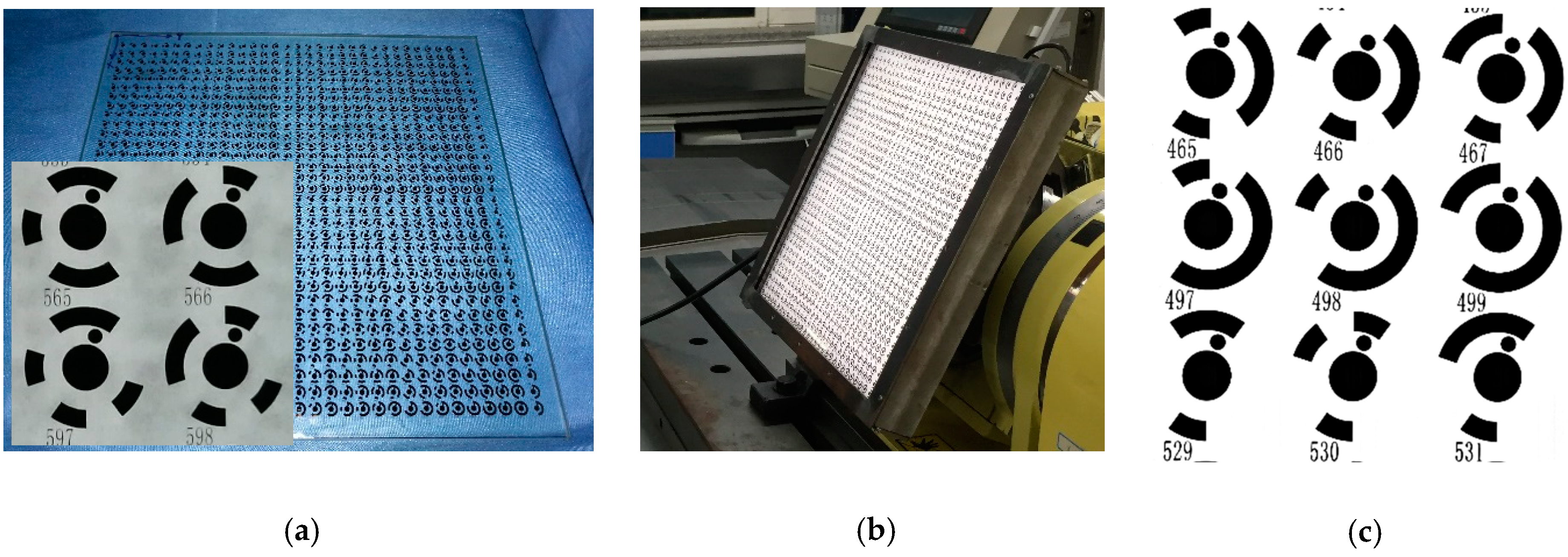
| Number of coding primitives | 1024 (see Figure 6a for detail) |
| Geometrical accuracy of single coded targets | <1 μm |
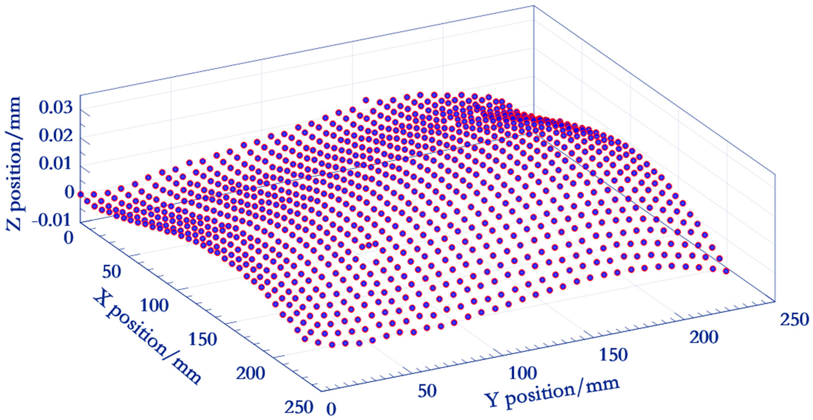
| Calibration accuracy of spatial geometric information | 0.5 μm |
| Camera Resolution | 5120 × 5120 pixels | 3072 × 3072 pixels | 1024 × 1024 pixels |
|---|---|---|---|
| The collected static image |  |  |  |
| Allowable maximum FPS | 33 FPS | 208 FPS | 308 FPS |
| FPS used in tests | 25 FPS | 100 FPS | 150 FPS |
| Subregion 1 | Subregion 2 | Subregion 3 | Subregion 4 | Entire Image | |
|---|---|---|---|---|---|
| Maximum distance error/pixel | 0.12 | 0.19 | 0.45 | 0.81 | 3.53 |
| Mean distance error/pixel | 0.07 | 0.06 | 0.11 | 0.24 | 0.27 |
| Object Plane /mm | Subregion | Distortion | ||||
|---|---|---|---|---|---|---|
| Observed (μm) | With Partition Model | Without Partition Model | ||||
| Calculated (μm) | Difference |C − O| (μm) | Calculated (μm) | Difference |C − O| (μm) | |||
| 428 mm | Subregion 1 (Radial distance = 13 mm) | − 0.31 | − 0.3 | 0.01 | − 0.34 | 0.03 |
| Subregion 2 (Radial distance = 26 mm) | − 20.25 | − 20.09 | 0.16 | − 17.63 | 2.62 | |
| Subregion 3 (Radial distance = 39 mm) | − 31.95 | − 30.85 | 1.1 | − 28.94 | 3.01 | |
| Subregion 4 (Radial distance = 52 mm) | − 37.35 | − 36.05 | 1.3 | − 32.67 | 4.68 | |
| 448 mm | Subregion 1 (Radial distance = 14 mm) | − 0.23 | − 0.22 | 0.01 | − 0.21 | 0.02 |
| Subregion 2 (Radial distance = 28 mm) | − 14.42 | − 13.78 | 0.64 | − 12.9 | 1.52 | |
| Subregion 3 (Radial distance = 42 mm) | − 24.31 | − 3.23 | 1.08 | − 21.83 | 2.48 | |
| Subregion 4 (Radial distance = 56 mm) | − 27.97 | − 26.22 | 1.75 | − 24.76 | 3.21 | |
© 2019 by the authors. Licensee MDPI, Basel, Switzerland. This article is an open access article distributed under the terms and conditions of the Creative Commons Attribution (CC BY) license (http://creativecommons.org/licenses/by/4.0/).
Share and Cite
Li, X.; Liu, W.; Pan, Y.; Ma, J.; Wang, F. A Knowledge-Driven Approach for 3D High Temporal-Spatial Measurement of an Arbitrary Contouring Error of CNC Machine Tools Using Monocular Vision. Sensors 2019, 19, 744. https://doi.org/10.3390/s19030744
Li X, Liu W, Pan Y, Ma J, Wang F. A Knowledge-Driven Approach for 3D High Temporal-Spatial Measurement of an Arbitrary Contouring Error of CNC Machine Tools Using Monocular Vision. Sensors. 2019; 19(3):744. https://doi.org/10.3390/s19030744
Chicago/Turabian StyleLi, Xiao, Wei Liu, Yi Pan, Jianwei Ma, and Fuji Wang. 2019. "A Knowledge-Driven Approach for 3D High Temporal-Spatial Measurement of an Arbitrary Contouring Error of CNC Machine Tools Using Monocular Vision" Sensors 19, no. 3: 744. https://doi.org/10.3390/s19030744
APA StyleLi, X., Liu, W., Pan, Y., Ma, J., & Wang, F. (2019). A Knowledge-Driven Approach for 3D High Temporal-Spatial Measurement of an Arbitrary Contouring Error of CNC Machine Tools Using Monocular Vision. Sensors, 19(3), 744. https://doi.org/10.3390/s19030744