High-Sensitivity Real-Time Tracking System for High-Speed Pipeline Inspection Gauge


Abstract
:
1. Introduction
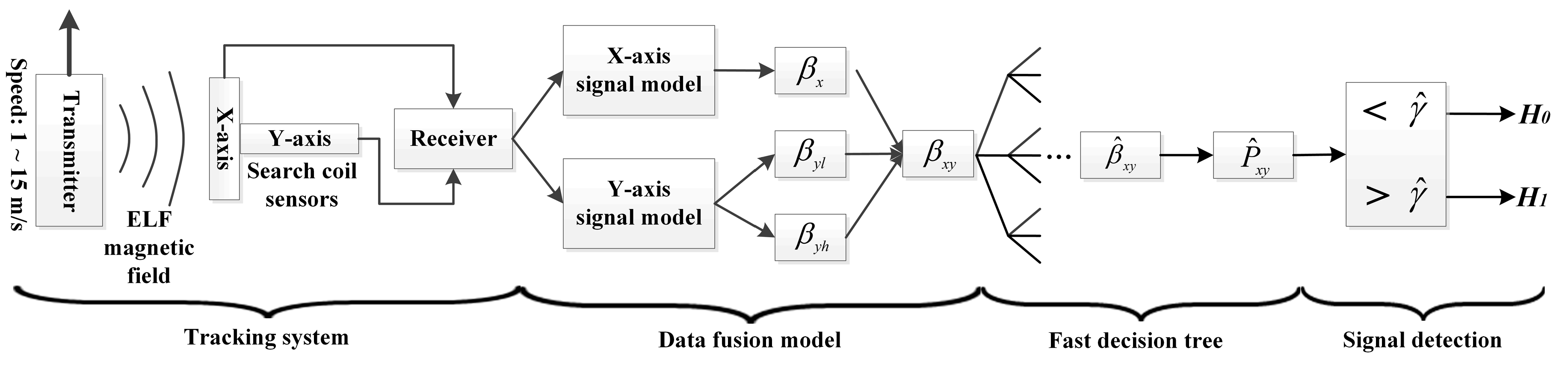
2. Simulation and Signal models
2.1. 2-D FEM Simulation Studies
2.2. Data Fusion Model
3. Fast decision Tree Method
4. Performance Evaluation
4.1. Detection Methods and Theoretical Bounds
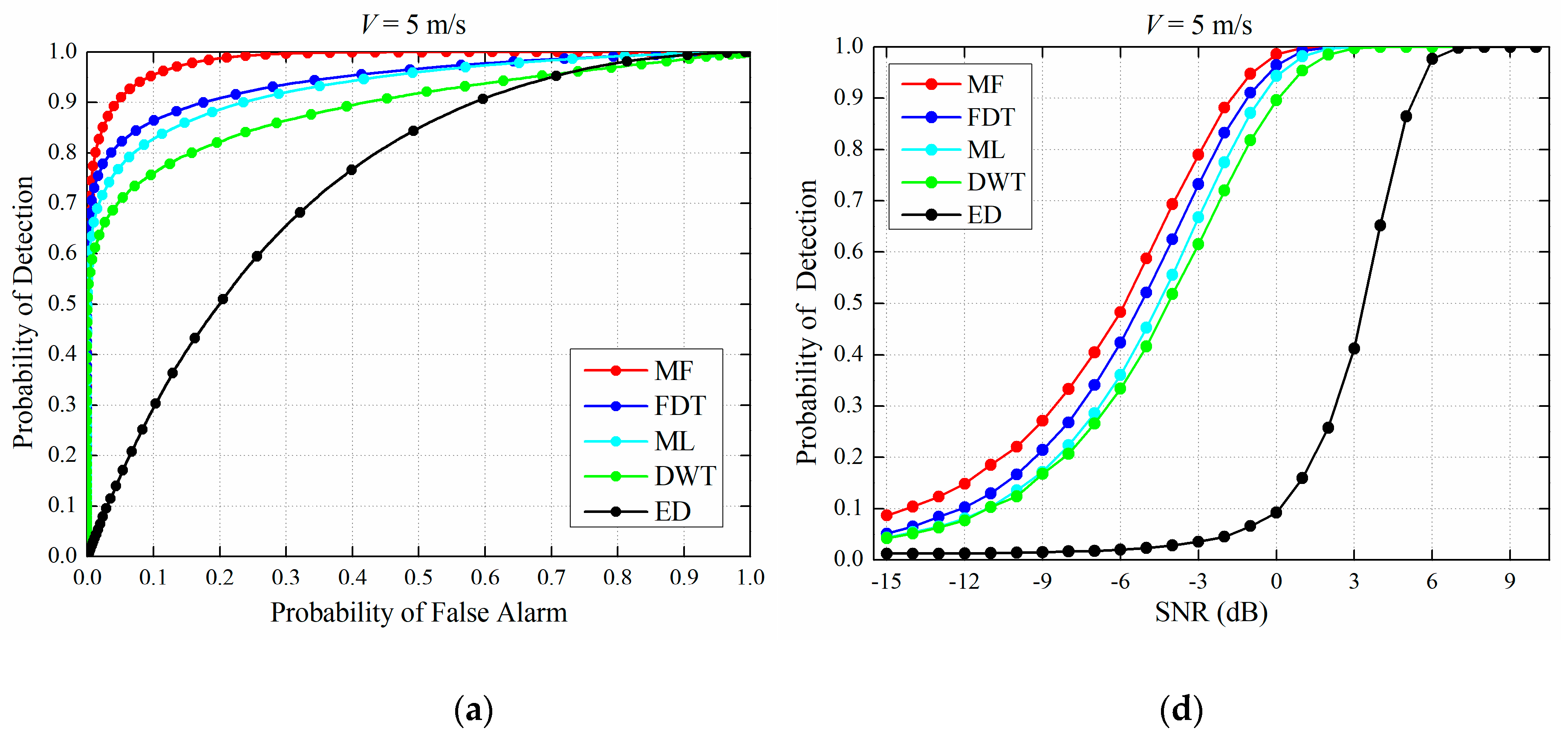
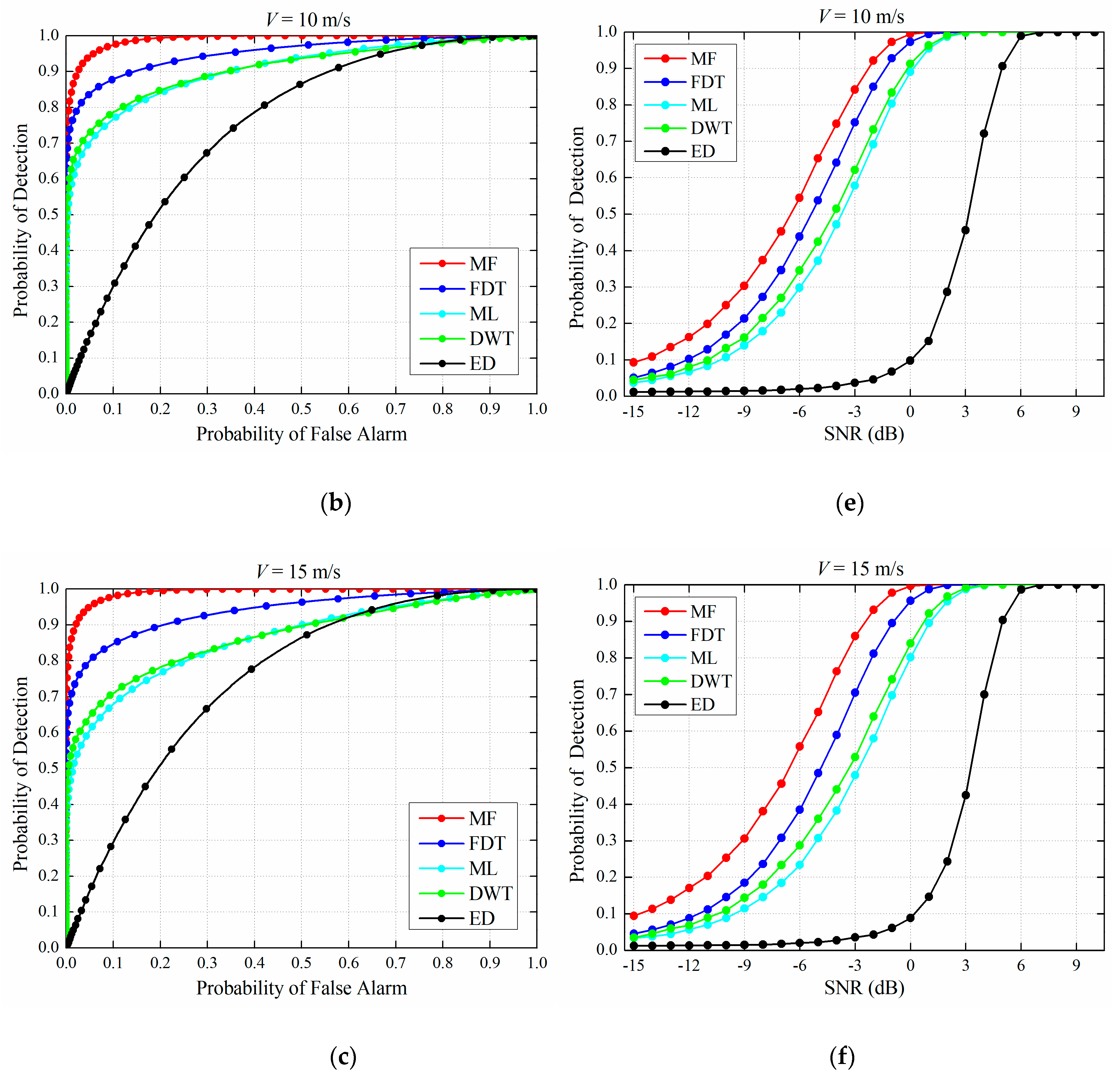
4.2. Monte Carlo Simulation Study
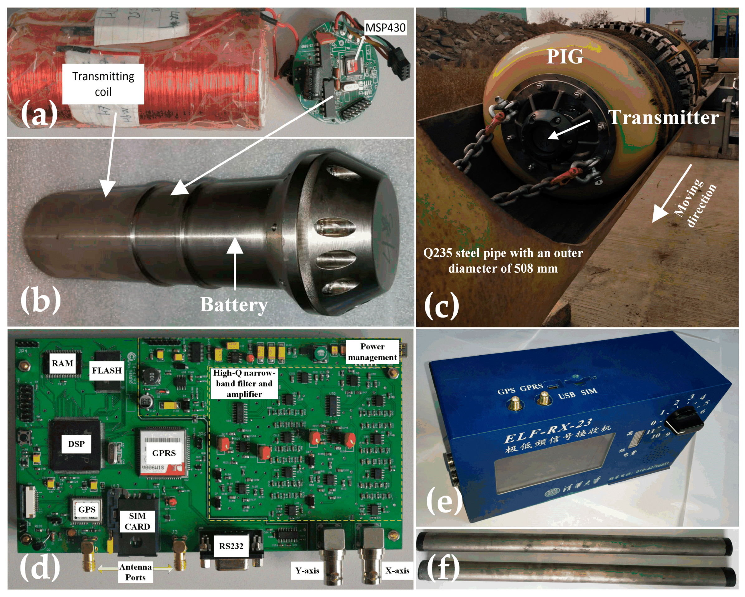
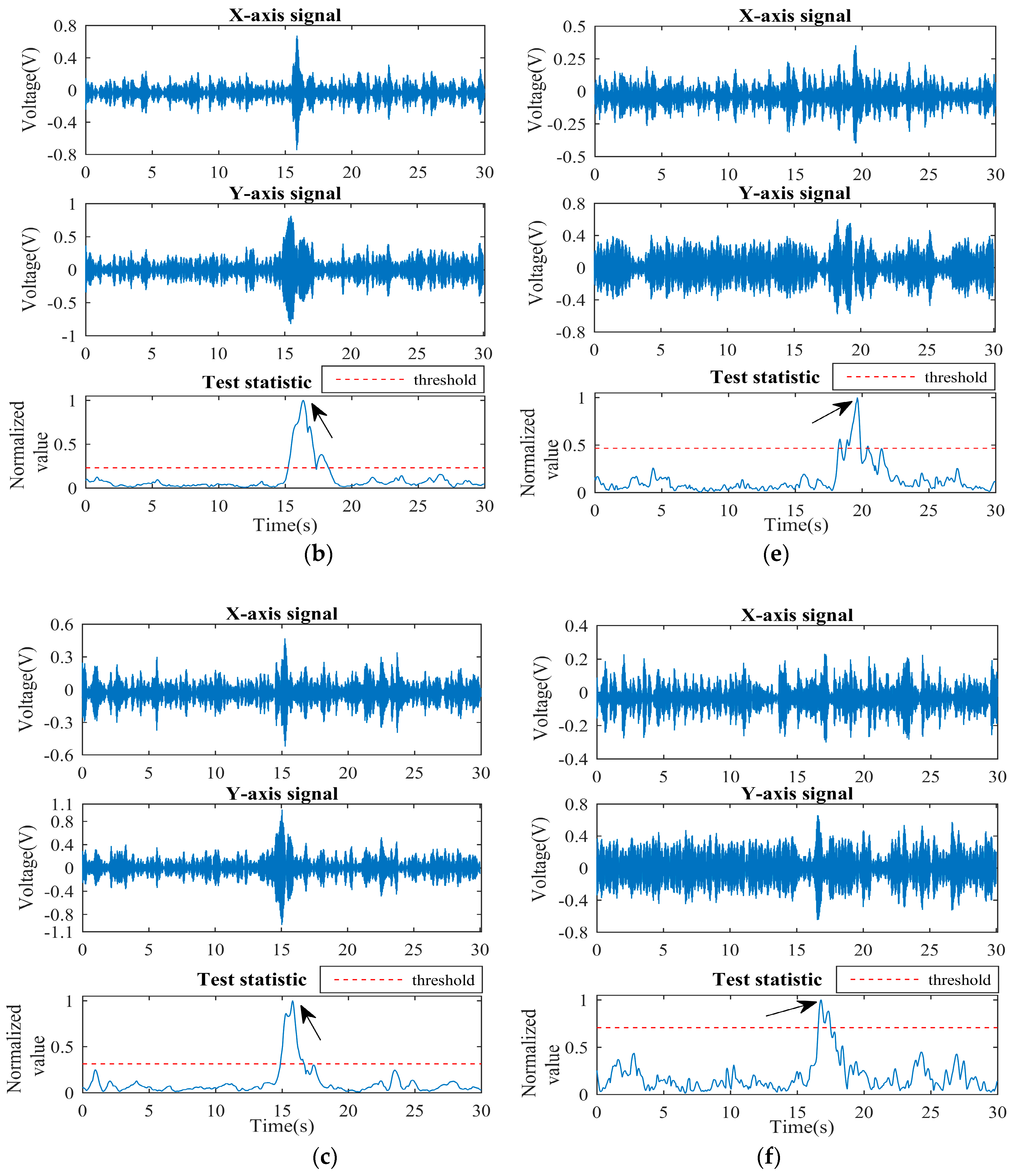
4.3. Field Testing and Validation
5. Discussions
6. Conclusions
Author Contributions
Funding
Conflicts of Interest
References
- Factbook, C.I.A. The World Factbook―Central Intelligence Agency. Available online: https://www.cia.gov/library/publications/the-world-factbook (accessed on 6 September 2016).
- Wu, J.; Kang, Y.; Tu, J.; Sun, Y. Analysis of the eddy-current effect in the Hi-speed axial MFL testing for steel pipe. Int. J. Appl. Electromagn. Mech. 2014, 45, 193–199. [Google Scholar] [CrossRef]
- Money, N. Dynamic speed control in high velocity pipelines. Pipeline Gas J. 2012, 239, 30–38. [Google Scholar]
- Sophian, A.; Tian, G.Y.; Fan, M. Pulsed eddy current non-destructive testing and evaluation: A review. Chinese J. Mech. Eng. 2017, 30, 500–514. [Google Scholar] [CrossRef]
- Araújo, R.P.; Freitas, V.C.G.; Lima, G.F.; Salazar, A.O.; Neto, A.D.D.; Maitelli, A.L. Pipeline Inspection Gauge’s Velocity Simulation Based on Pressure Differential Using Artificial Neural Networks. Sensors 2018, 18, 3072. [Google Scholar] [CrossRef] [PubMed]
- Feng, Q.; Li, R.; Nie, B.; Liu, S.; Zhao, L.; Zhang, H. Literature Review: Theory and Application of In-Line Inspection Technologies for Oil and Gas Pipeline Girth Weld Defection. Sensors 2016, 17, 50. [Google Scholar] [CrossRef] [PubMed]
- Orasheva, J. The Effect of Corrosion Defects on the Failure of Oil and Gas Transmission Pipelines: A Finite Element Modeling Study. Master’s Thesis, University of North Florida, Jacksonville, FL, USA, 2017. [Google Scholar]
- Santos-Ruiz, I.; Bermúdez, J.R.; López-Estrada, F.R.; Puig, V.; Torres, L.; Delgado-Aguiñaga, J.A. Online leak diagnosis in pipelines using an EKF-based and steady-state mixed approach. Control Eng. Pract. 2018, 81, 55–64. [Google Scholar] [CrossRef]
- Zhou, Z.H.; Chen, G.H. Challenges to Risk Management of Underground Transmission Hazardous Material Pipelines in China. Proc. Eng. 2015, 130, 1503–1513. [Google Scholar] [CrossRef]
- Significant Incidents, Pipeline Hazardous Materials Safety Administration, United States Department of Transportation. Available online: https://opsweb.phmsa.dot.gov/primis_pdm/significant_inc_trend.asp (accessed on 31 December 2018).
- Khodayari-Rostamabad, A.; Reilly, J.P.; Nikolova, N.K.; Hare, J.R.; Pasha, S. Machine learning techniques for the analysis of magnetic flux leakage images in pipeline inspection. IEEE Trans. Magn. 2009, 45, 3073–3084. [Google Scholar] [CrossRef]
- Timashev, S.; Bushinskaya, A. Diagnostics and reliability of pipeline systems; Springer International Publishing: Cham, Switzerland, 2016; p. 30. [Google Scholar]
- Kim, H.M.; Park, G.S. A New Sensitive Excitation Technique in Nondestructive Inspection for Underground Pipelines by Using Differential Coils. IEEE Trans. Magn. 2017, 53, 1–4. [Google Scholar] [CrossRef]
- Rodríguez-Olivares, N.; Cruz-Cruz, J.; Gómez-Hernández, A.; Hernández-Alvarado, R.; Nava-Balanzar, L.; Salgado-Jiménez, T.; Soto-Cajiga, J. Improvement of Ultrasonic Pulse Generator for Automatic Pipeline Inspection. Sensors 2018, 18, 2950. [Google Scholar] [CrossRef]
- Miro, J.V.; Hunt, D.; Ulapane, N.; Behrens, M. Towards Automatic Robotic NDT Dense Mapping for Pipeline Integrity Inspection. Field Serv. Robot. Springer Proc. Adv. Robot. 2018, 5, 319–333. [Google Scholar]
- Piao, G.; Guo, J.; Hu, T.; Leung, H.; Deng, Y. Fast reconstruction of 3-D defect profile from MFL signals using key physics-based parameters and SVM. NDT&E Int. 2019, 103, 26–38. [Google Scholar]
- Sun, L.; Li, Y.; Du, G.; Wang, W.; Zhang, Y. Modification design of high-precision above ground marking system. In Proceedings of the IEEE Chinese Control and Decision Conference, Xuzhou, China, 26–28 May 2010; pp. 531–535. [Google Scholar]
- Wu, X.; Xu, A.; Xiao, Y.; Zhou, B.; Wang, G.; Zeng, R. Research on Above Ground Marker System of pipeline Internal Inspection Instrument Based on geophone array. In Proceedings of the IEEE 6th International Conference on Wireless Communications Networking and Mobile Computing, Chengdu, China, 23–25 September 2010; pp. 1–4. [Google Scholar]
- Yan, S.; Zhang, C.; Li, R.; Cai, M.; Jia, G. Theory and Application of Magnetic Flux Leakage Pipeline Detection. Sensors 2015, 15, 31036–31055. [Google Scholar]
- Sahli, H.; El-Sheimy, N. A Novel Method to Enhance Pipeline Trajectory Determination Using Pipeline Junctions. Sensors 2016, 16, 567. [Google Scholar] [CrossRef]
- Li, Y.; Wang, D.; Sun, L. A novel algorithm for acoustic above ground marking based on function fitting. Measurement 2013, 46, 2341–2347. [Google Scholar] [CrossRef]
- Li, Y.; Liu, S.; Dorantes-Gonzalez, D.J.; Zhou, C.; Zhu, H. A novel above-ground marking approach based on the girth weld impact sound for pipeline defect inspection. Insight Non Destr. Test Cond. Monit. 2014, 56, 677–682. [Google Scholar] [CrossRef]
- Song, X.; Jian, Z.; Zhang, G. New Research on MEMS acoustic vector sensors used in pipeline ground markers. Sensors 2015, 15, 274–284. [Google Scholar] [CrossRef]
- Sun, L.; Li, Y.; Wu, Y. Establishment of theoretical model of magnetic dipole for ground marking system. In Proceedings of the IEEE Conference on Control and Decision, Chongqing, China, 28–30 May 2017; pp. 6134–6138. [Google Scholar]
- Su, Z.; Huang, S.; Zhao, W.; Wang, S.; Feng, H.; Chen, J. Development of a Portable High-Precision Above Ground Marker System for an MFL Pipeline Inspector. In Proceedings of the 18th World Conference on Nondestructive Testing, Durban, South Africa, April 2012; pp. 16–20. [Google Scholar]
- Guo, J.; Tan, B.; Cai, X. Estimation and detection of the weak transient ELF signal based on the phase inverting double-peak exponential model. Chinese J. Sci. Instrum. 2015, 36, 1682–1691. [Google Scholar]
- Chen, S.; Guo, J.; Hu, T. Distribution and detection of ELF weak magnetic field in ferromagnetic pipeline environment. Chinese J. Sci. Instrum. 2011, 32, 2348–2356. [Google Scholar]
- Qi, H.; Ye, J.; Zhang, X.; Chen, H. Wireless tracking and locating system for in-pipe robot. Sens. Actuators A Phys. 2010, 159, 117–125. [Google Scholar] [CrossRef]
- Piao, G.; Guo, J.; Hu, T. A novel real-time detection of orthogonal transient weak ELF magnetic signals. In Proceedings of the IEEE Sensors Applications Symposium, Glassboro, NJ, USA, 13–15 March 2017; pp. 494–499. [Google Scholar]
- Qi, H.; Zhang, X.; Chen, H. Tracing and localization system for pipeline robot. Mechatronics 2009, 19, 76–84. [Google Scholar] [CrossRef]
- Guo, J.; Cai, X.; Hu, T. Key technologies of tracking and positioning of intelligent robots in oil and gas pipelines: A review of recent advances. Chinese J. Sci. Instrum. 2015, 36, 481–498. [Google Scholar]
- Lenz, J.; Edelstein, S. Magnetic sensors and their applications. IEEE Sens. J. 2006, 6, 631–649. [Google Scholar] [CrossRef]
- Ripka, P.; Janosek, M. Advances in magnetic field sensors. IEEE Sens. J. 2010, 10, 1108–1116. [Google Scholar] [CrossRef]
- Kay, S.M. Fundamentals of Statistical Signal Processing: Detection Theory; Prentice-Hall: Upper Saddle River, NJ, USA, 1998. [Google Scholar]
- Levy, B.C. Principles of Signal Detection and Parameter Estimation; Cambridge University Press: Cambridge, UK, 2008. [Google Scholar]
- Poor, H.V.; Hadjiliadis, O. Quickest Detection; Cambridge University Press: Cambridge, UK, 2008. [Google Scholar]
- Liang, W.; Que, P. Optimal scale wavelet transform for the identification of weak ultrasonic signals. Measurement 2009, 42, 164–169. [Google Scholar] [CrossRef]
- Gómez, M.J.; Castejón, C.; Garcia-Prada, J.C. Review of Recent Advances in the Application of the Wavelet Transform to Diagnose Cracked Rotors. Algorithms 2016, 9, 19. [Google Scholar] [CrossRef]
- Bermúdez, J.R.; López-Estrada, F.R.; Besançon, G.; Valencia-Palomo, G.; Torres, L.; Hernández, H.R. Modeling and Simulation of a Hydraulic Network for Leak Diagnosis. Math. Comput. Appl. 2018, 23, 70. [Google Scholar] [CrossRef]
- Birsan, M. Measurement of the extremely low frequency (ELF) magnetic field emission from a ship. Meas. Sci. Technol. 2011, 22, 085709. [Google Scholar] [CrossRef]
- Qin, Y.; Xing, J.; Mao, Y. Weak transient fault feature extraction based on an optimized Morlet wavelet and kurtosis. Meas. Sci. Technol. 2016, 27, 085003. [Google Scholar] [CrossRef]
- Bozchalooi, I.S.; Liang, M. Parameter-free bearing fault detection based on maximum likelihood estimation and differentiation. Meas. Sci. Technol. 2009, 20, 065102. [Google Scholar] [CrossRef]
- Cai, X.; Guo, J.; Hu, T.; Zhang, Z.; Chen, S. Reverse optimization design of ELF magnetic transmitter for ferromagnetic pipeline. Chinese J. Sci. Instrument 2014, 35, 634–641. [Google Scholar]


| Property | Iron Core | Coil | Oil | Q235 Steel Pipe | Soil | Air |
|---|---|---|---|---|---|---|
| Conductivity (S/m) | 1 × 10⁷ | 5.7 × 10⁷ | 0.01 | 2 × 10⁶ | 0.005 | 0 |
| Permeability (H/m) | 1000 µ0 1 | µ0 | µ0 | 500 µ0 | µ0 | µ0 |
| Mesh size (m) | 0.01 | 0.01 | 0.1 | 0.02 | 0.2 | 0.2 |
| Property | Value |
|---|---|
| Length of pipeline (L) | 45 m |
| Burial depth (DB) | 2.5~5 m |
| Outer radius of pipeline (R) | 254 mm |
| Thickness of pipe wall (T) | 6~15 mm |
| Inner radius of pipeline | (R-T) mm |
| Length of coil (LC) | 130 mm |
| Width of transmitting coil (2WC) | 59 mm |
| Width of iron core (2WI) | 25 mm |
| Coil turns | 25,000 |
| Transmitting current (RMS) | 4 mA |
| Current frequency | 23 Hz |
| Speed of transmitter (V) | 1~15 m/s |
| Notations | Description |
|---|---|
| Nx | Number of samples of X-axis ELF signal |
| Ny | Number of samples of Y-axis ELF signal |
| βxy | Fused envelope decay rate |
| Estimated fused enveloped decay rate | |
| βmax | Fused envelope decay rate corresponding to maximum speed of transmitter |
| Hx | Observation matrix of X-axis ELF signal |
| Maximized orthogonal signal power | |
| Energy of X-axis observation vector | |
| Energy of Y-axis observation vector | |
| η | Normalized signal energy |
| Cm | Computation cost of multiplication |
| Ca | Computation cost of addition |
| Threshold for signal detection |
| L | V = 5 m/s, βxy = 5.5 | V = 10 m/s, βxy = 21.2 | V = 15 m/s, βxy = 46.9 | |||||||
|---|---|---|---|---|---|---|---|---|---|---|
| 1 | 8.4 | 25.2 | 42 | 8.4 | 25.2 | 42 | 8.4 | 25.2 | 43 | |
| η | 0.9839 | 0.8184 | 0.6975 | 0.9104 | 0.9679 | 0.9234 | 0.7881 | 0.9032 | 0.9303 | |
| 2 | 2.8 | 8.4 | 14 | 19.6 | 25.2 | 30.8 | 36.4 | 42 | 47.6 | |
| η | 0.9703 | 0.9839 | 0.9288 | 0.9704 | 0.9679 | 0.9568 | 0.9261 | 0.9303 | 0.9313 | |
| 3 | 6.53 | 8.4 | 10.27 | 17.73 | 19.6 | 21.47 | 45.73 | 47.6 | 49.47 | |
| η | 0.9946 | 0.9839 | 0.9676 | 0.9681 | 0.9704 | 0.9709 | 0.9312 | 0.9313 | 0.9310 | |
| 4 | 5.9 | 6.53 | 7.16 | 20.84 | 21.47 | 22.09 | 46.98 | 47.6 | 48.2 | |
| η | 0.9956 | 0.9946 | 0.9920 | 0.9709 | 0.9709 | 0.9707 | 0.9513 | 0.9513 | 0.9512 | |
| Δη | 0.9956 − 0.9946 = 0.001 | 0.9709 − 0.9709 < 0.0001 | 0.9513 − 0.9513 < 0.0001 | |||||||
| Δβxy1 | 5.9 − 5.5 = 0.40 | 21.47 − 21.2 = 0.27 | 47.6 − 46.9 = 0.70 | |||||||
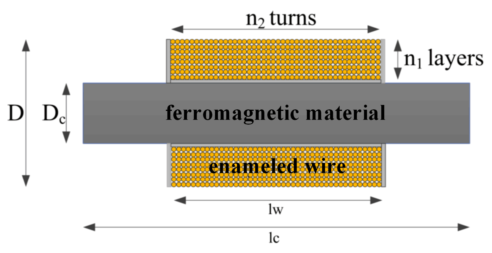
| D (mm) | Dc (mm) | n2 | n1 | lw (mm) | lc (mm) |
|---|---|---|---|---|---|
| 30 | 20 | 2400 | 23 | 720 | 800 |
| Figure 10 | Pipe Wall Thickness | True Speed | Estimated Speed | Estimated SNR |
|---|---|---|---|---|
| (a) | 10 mm | 4.7 m/s | 4.9 m/s | 10.35 dB |
| (b) | 10 mm | 8.0 m/s | 7.6 m/s | 9.45 dB |
| (c) | 10 mm | 11.1 m/s | 10.1 m/s | 6.95 dB |
| (d) | 15 mm | 6.1 m/s | 6 m/s | 4.00 dB |
| (e) | 15 mm | 8.3 m/s | 7.8 m/s | 0.55 dB |
| (f) | 15 mm | 12.5 m/s | 13.8 m/s | −0.9 dB |
© 2019 by the authors. Licensee MDPI, Basel, Switzerland. This article is an open access article distributed under the terms and conditions of the Creative Commons Attribution (CC BY) license (http://creativecommons.org/licenses/by/4.0/).
Share and Cite
Piao, G.; Guo, J.; Hu, T.; Deng, Y. High-Sensitivity Real-Time Tracking System for High-Speed Pipeline Inspection Gauge. Sensors 2019, 19, 731. https://doi.org/10.3390/s19030731
Piao G, Guo J, Hu T, Deng Y. High-Sensitivity Real-Time Tracking System for High-Speed Pipeline Inspection Gauge. Sensors. 2019; 19(3):731. https://doi.org/10.3390/s19030731
Chicago/Turabian StylePiao, Guanyu, Jingbo Guo, Tiehua Hu, and Yiming Deng. 2019. "High-Sensitivity Real-Time Tracking System for High-Speed Pipeline Inspection Gauge" Sensors 19, no. 3: 731. https://doi.org/10.3390/s19030731
APA StylePiao, G., Guo, J., Hu, T., & Deng, Y. (2019). High-Sensitivity Real-Time Tracking System for High-Speed Pipeline Inspection Gauge. Sensors, 19(3), 731. https://doi.org/10.3390/s19030731