Predicting Depth from Single RGB Images with Pyramidal Three-Streamed Networks


Abstract
:1. Introduction
2. Related Work
3. Methodology
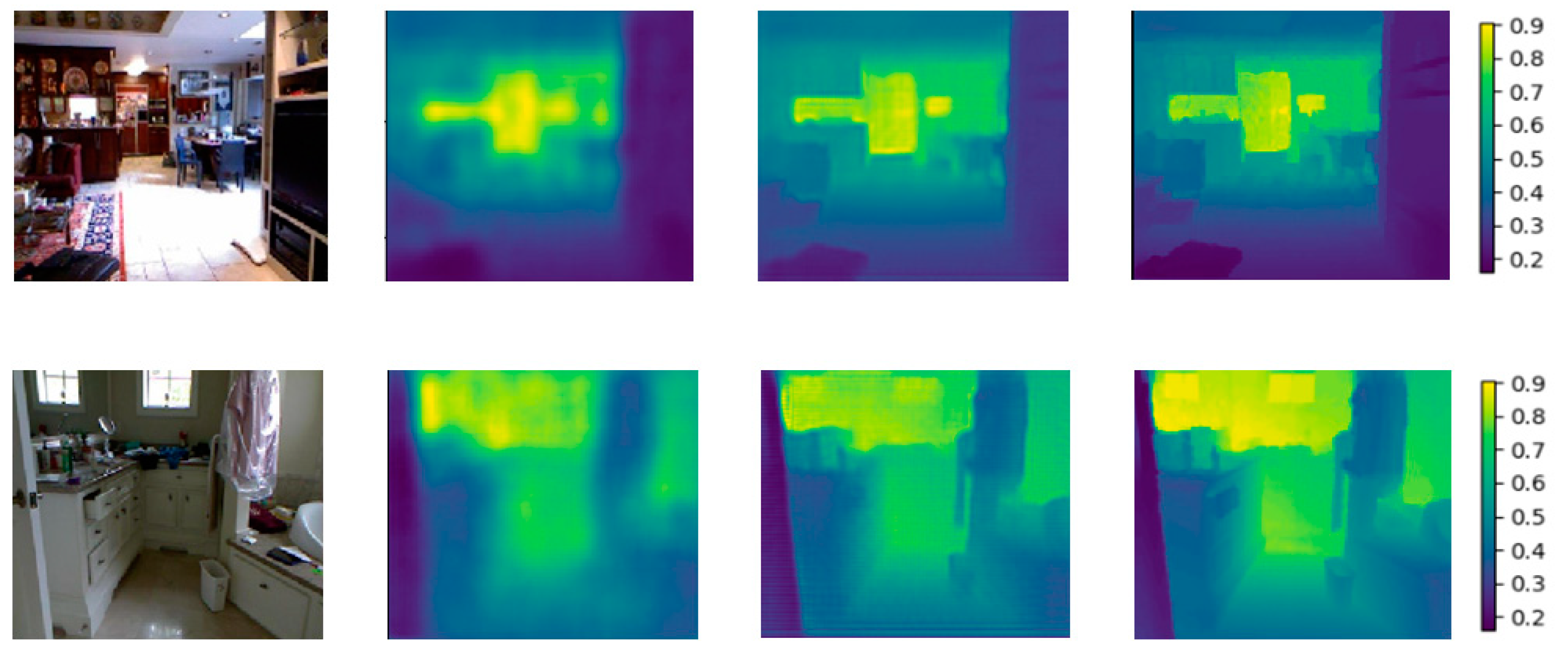
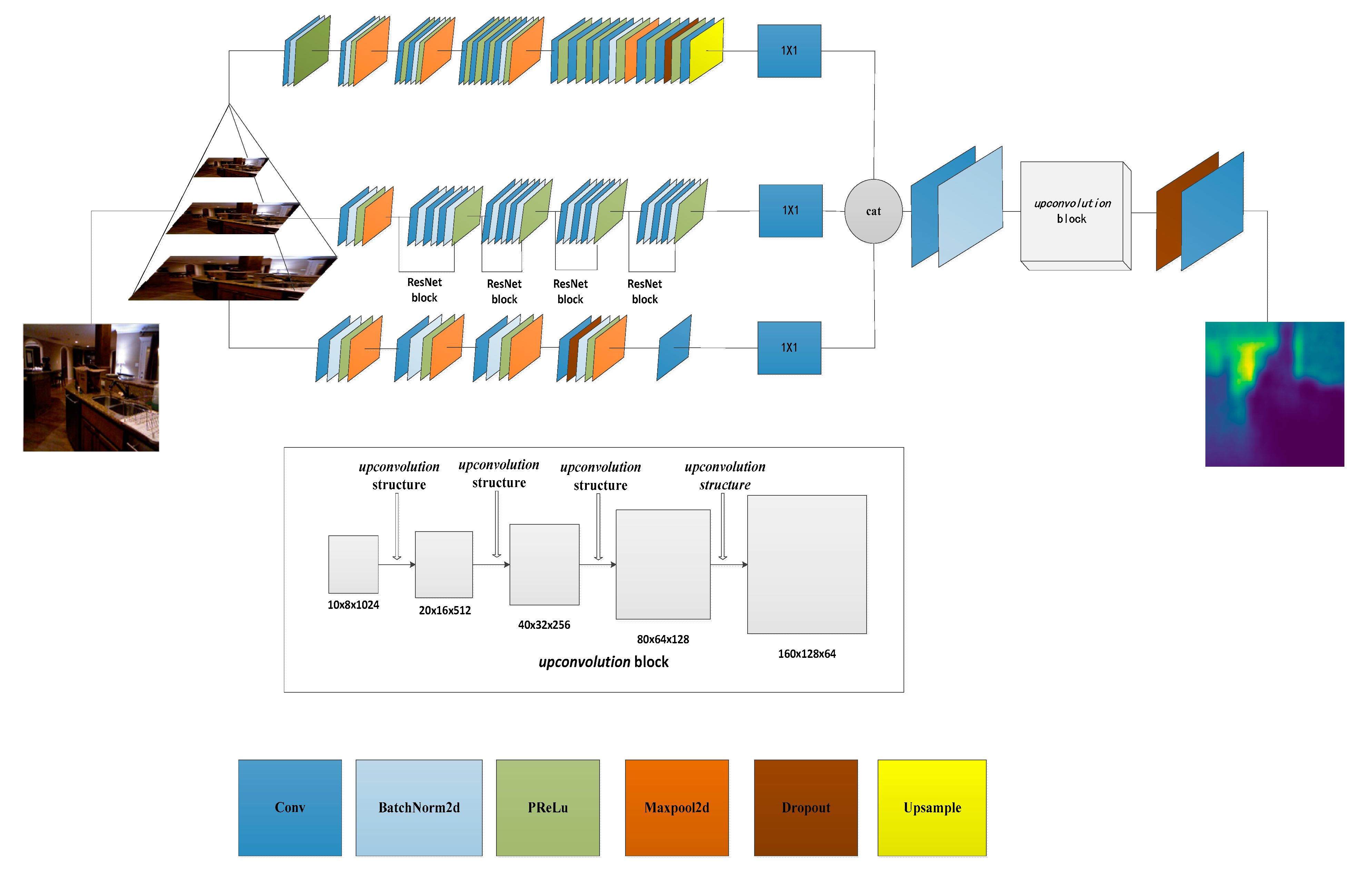
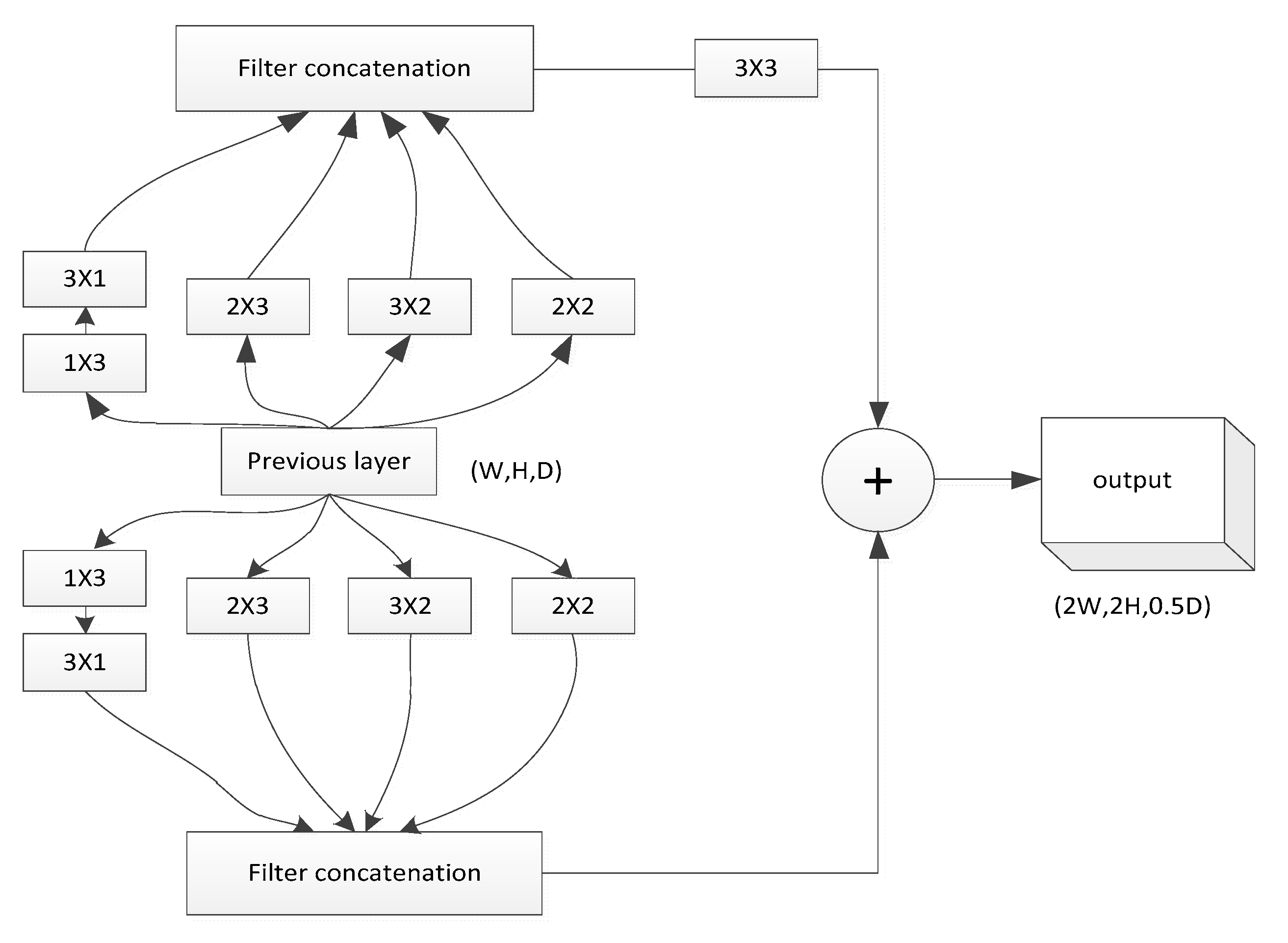
3.1. Network Architecture
3.2. Data Augmentation
3.3. Loss Function
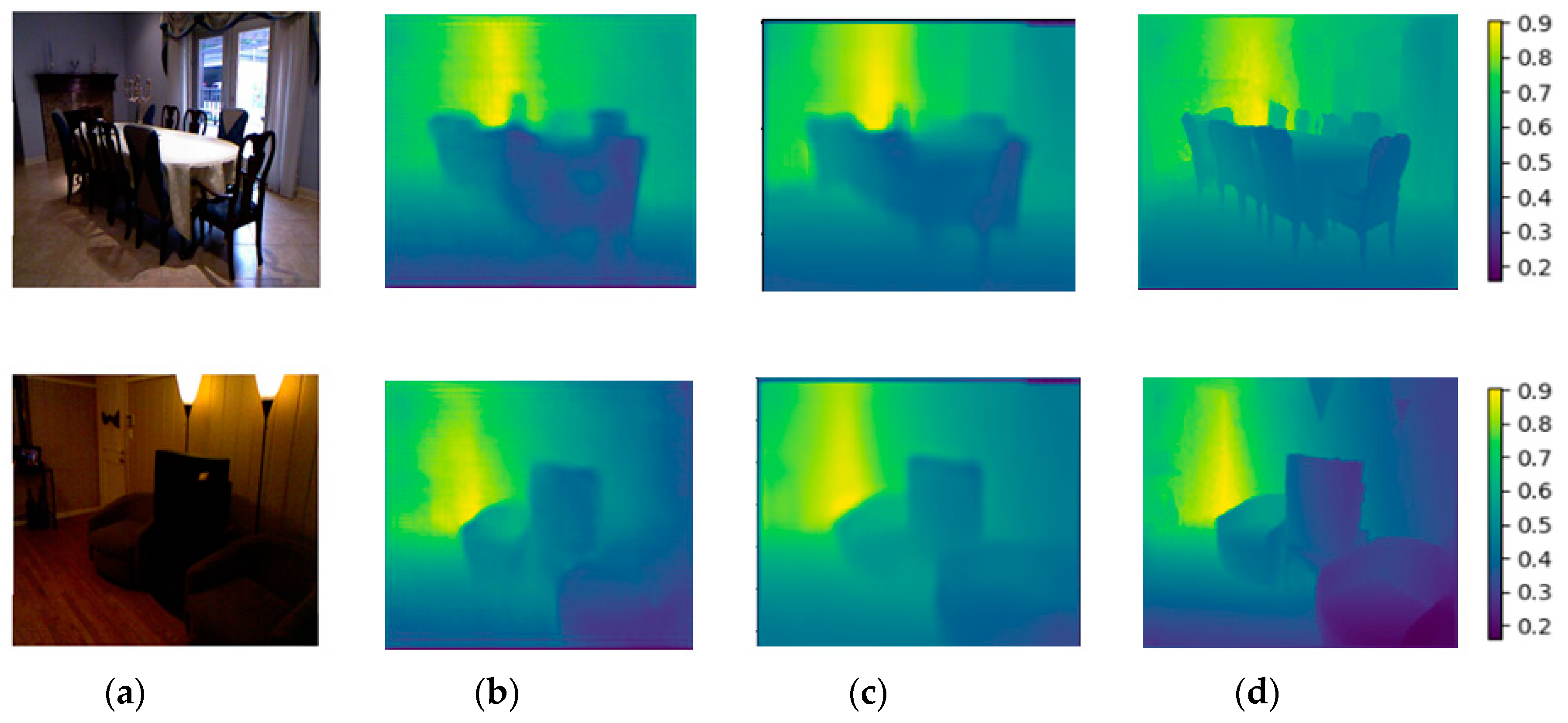
4. Experimentation
4.1. Dataset
4.2. Baselines and Comparisons
- Threshold: % of s.t.
- Mean relative error (rel):
- Mean Error (log10):
- Root mean squared error(rms):
- Root mean squared error(rms(log)):
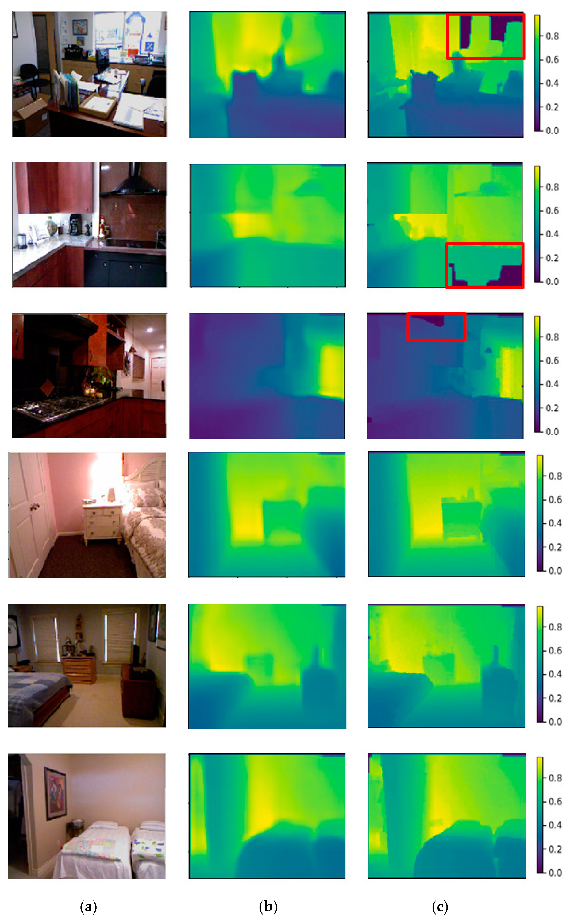
5. Discussion and Conclusion
Author Contributions
Funding
Acknowledgments
Conflicts of Interest
References
- Wang, S.; Zuo, X.; Wang, R.; Cheng, F.; Yang, R. A generative human-robot motion retargeting approach using a single depth sensor. In Proceedings of the IEEE International Conference on Robotics and Automation (ICRA), Singapore, 29 May–3 June 2017; pp. 5369–5376. [Google Scholar]
- Ragaglia, M.; Zanchettin, A.M.; Rocco, P. Trajectory generation algorithm for safe human-robot collaboration based on multiple depth sensor measurements. Mechatronics 2018, 55, 267–281. [Google Scholar] [CrossRef]
- Wang, H.; Wang, G.; Wang, X.; Ruan, C.; Chen, S. A kind of infrared expand depth of field vision sensor in low-visibility road condition for safety-driving. Sens. Rev. 2016, 36, 7–13. [Google Scholar] [CrossRef]
- Hong, Z.; Ai, Q.; Chen, K. Line-laser-based visual measurement for pavement 3D rut depth in driving state. Electron. Lett. 2018, 54, 1172–1174. [Google Scholar] [CrossRef]
- Chen, Y.; Yang, D.; Liao, W. Efficient multi-view 3D video multicast with depth image-based rendering in LTE networks. In Proceedings of the IEEE Global Communications Conference (GLOBECOM), Atlanta, GA, USA, 9–13 December 2013; pp. 4427–4433. [Google Scholar]
- Cao, Y.; Xu, B.; Ye, Z.; Yang, J.; Cao, Y.; Tisse, C.; Li, X. Depth and thermal sensor fusion to enhance 3D thermographic reconstruction. Opt. Express 2018, 26, 8179–8193. [Google Scholar] [CrossRef] [PubMed]
- Song, H.; Choi, W.; Kim, H. Robust Vision-Based Relative-Localization Approach Using an RGB-Depth Camera and LiDAR Sensor Fusion. IEEE Trans. Ind. Electron. 2016, 63, 3725–3736. [Google Scholar] [CrossRef]
- Omelina, L.; Jansen, B.; Bonnechere, B.; Oravec, M.; Pavlovicova, J.; Jan, S.V. Interaction Detection with Depth Sensing and Body Tracking Cameras in Physical Rehabilitation. Method Inf. Med. 2016, 55, 70–78. [Google Scholar]
- Kepski, M.; Kwolek, B. Event-driven system for fall detection using body-worn accelerometer and depth sensor. IET Comput. Vis. 2018, 12, 48–58. [Google Scholar] [CrossRef]
- Akbarally, H.; Kleeman, L. 3D robot sensing from sonar and vision. In Proceedings of the IEEE International Conference on Robotics and Automation, Minneapolis, MN, USA, 22–28 April 1996; pp. 686–691. [Google Scholar]
- Pieraccini, M.; Luzi, G.; Mecatti, D.; Noferini, L.; Atzeni, C. A microwave radar technique for dynamic testing of large structures. IEEE Trans. Microw. Theory 2003, 51, 1603–1609. [Google Scholar] [CrossRef]
- Memisevic, R.; Conrad, C. Stereopsis via deep learning. In Proceedings of the Neural Information Processing Systems 2011 (NIPS 2011), Granada, Spain, 11–12 December 2011; pp. 1–2. [Google Scholar]
- Sinz, F.H.; Candela, J.Q.; Bakir, G.H.; Rasmussen, C.E.; Franz, M.O. Learning depth from stereo. Jt. Pattern Recognit. Symp. 2004, 3175, 245–252. [Google Scholar]
- Szeliski, R. Structure from Motion. Computer Vision; Springer: London, UK, 2011; pp. 303–334. [Google Scholar]
- Chen, Y.; Wu, Y.; Liu, C.; Sun, W.; Chen, Y. Depth map generation based on depth from focus. In Proceedings of the IEEE Conference on Electronic Devices, Systems and Applications (ICEDSA), Kuala Lumpur, Malaysia, 11–14 April 2010; pp. 59–63.
- Favaro, P. Recovering thin structures via nonlocal-means regularization with application to depth from defocus. In Proceedings of the IEEE Conference on Computer Vision and Pattern Recognition (CVPR), San Francisco, CA, USA, 13–18 June 2010; pp. 1133–1140. [Google Scholar]
- Zhuo, S.J.; Sim, T. Defocus map estimation from a single image. Lect. Notes Comput. Sc. 2011, 44, 1852–1858. [Google Scholar] [CrossRef]
- Silberman, N.; Hoiem, D.; Kohli, P.; Fergus, R. Indoor segmentation and support inference from RGBD images. In Proceedings of the IEEE Conference on European Conference on Computer Vision (ECCV), Florence, Italy, 7–13 October 2012; pp. 746–760. [Google Scholar]
- Karsch, K.; Liu, C.; Kang, S.B. Depth Extraction from Video Using Non-parametric Sampling. In Proceedings of the IEEE Conference on European Conference on Computer Vision (ECCV), Florence, Italy, 7–13 October 2012; pp. 775–788. [Google Scholar]
- Liu, M.; Salzmann, M.; He, X. Discrete-Continuous Depth Estimation from a Single Image. In Proceedings of the IEEE Conference on Computer Vision and Pattern Recognition (CVPR), Columbus, OH, USA, 24–27 June 2014; pp. 716–723. [Google Scholar]
- Saxena, A.; Chung, S.; Ng, A.Y. Learning depth from single monocular images. In Proceedings of the International Conference on Neural Information Processing Systems (NIPS), Vancouver, BC, Canada, 5–6 December 2006; pp. 1161–1168. [Google Scholar]
- Saxena, A.; Sun, M.; Ng, A.Y. Make3D: Learning 3D Scene Structure from a Single Still Image. IEEE Trans. Pattern Anal. Mach. Intell. 2009, 31, 824–840. [Google Scholar] [CrossRef] [PubMed]
- Liu, B.; Gould, S.; Koller, D. Single Image Depth Estimation from Predicted Semantic Labels. In Proceedings of the IEEE Conference on Computer vision and pattern recognition (CVPR), San Francisco, CA, USA, 13–18 June 2010; pp. 1253–1260. [Google Scholar]
- Hoiem, D.; Efros, A.A.; Hebert, M. Geometric Context from a single image. In Proceedings of the International Conference on Computer Vision (ICCV), Beijing, China, 17–20 October 2005; pp. 654–661. [Google Scholar]
- Eigen, D.; Puhrsch, C.; Fergus, R. Depth Map Prediction from a Single Image Using a Multi-Scale Deep Network. In Proceedings of the International Conference on Neural Information Processing Systems (NIPS), Montréal, QC, Canada, 8–13 December 2014; pp. 2366–2374. [Google Scholar]
- Eigen, D.; Fergus, R. Predicting Depth, Surface Normals and Semantic Labels with a Common Multi-scale Convolutional Architecture. In Proceedings of the IEEE Conference on Computer vision and pattern recognition (CVPR), Boston, MA, USA, 8–12 June 2015; pp. 2650–2658. [Google Scholar]
- Liu, F.Y.; Shen, C.H.; Lin, G.S.; Reid, I. Learning Depth from Single Monocular Images Using Deep Convolutional Neural Fields. IEEE Trans. Pattern Anal. 2016, 38, 2024–2039. [Google Scholar] [CrossRef] [PubMed]
- Roy, A.; Todorovic, S. Monocular Depth Estimation Using Neural Regression Forest. In Proceedings of the IEEE Conference on Computer vision and pattern recognition (CVPR), Las Vegas, NV, USA, 26 June–1 July 2016; pp. 5506–5514. [Google Scholar]
- Wang, P.; Shen, X.; Lin, Z.; Cohen, S.; Price, B.; Yuille, A.L. Towards unified depth and semantic prediction from a single image. In Proceedings of the IEEE Conference on Computer vision and pattern recognition (CVPR), Boston, MA, USA, 8–12 June 2015; pp. 2800–2809. [Google Scholar]
- Laina, I.; Rupprecht, C.; Belagiannis, V.; Tombari, F.; Navab, N. Deeper Depth Prediction with Fully Convolutional Residual Networks. In Proceedings of the Fourth International Conference on 3D Vision (3DV), Stanford, CA, USA, 25–28 October 2016; pp. 239–248. [Google Scholar]
- Li, B.; Shen, C.; Dai, Y.; Van Den Hengel, A.; He, M. Depth and surface normal estimation from monocular images using regression on deep features and hierarchical CRFs. In Proceedings of the IEEE Conference on Computer Vision and Pattern Recognition (CVPR), Boston, MA, USA, 7–12 June 2015; pp. 1119–1127. [Google Scholar]
- Krizhevsky, A.; Sutskever, I.; Hinton, G.E. ImageNet Classification with Deep Convolutional Neural Networks. In Proceedings of the International Conference on Neural Information Processing Systems, Doha, Qatar, 12–15 November 2012; pp. 1097–1105. [Google Scholar]
- Chakrabarti, A.; Shao, J.; Shakhnarovich, G. Depth from a Single Image by Harmonizing Overcomplete Local Network Predictions. In Proceedings of the Annual Conference on Neural Information Processing Systems, Barcelona, Spain, 5–10 December 2016; pp. 2658–2666. [Google Scholar]
- Levin, A.; Fergus, R.; Freeman, W.T. Image and depth from a conventional camera with a coded aperture. ACM Trans. Graphics 2007, 26, 70. [Google Scholar] [CrossRef]
- He, K.; Zhang, X.; Ren, S.; Sun, J. Delving Deep into Rectifiers: Surpassing Human-Level Performance on ImageNet Classification. In Proceedings of the IEEE international conference on computer vision (ICCV), Santiago, Chile, 13–16 December 2015; pp. 1026–1034. [Google Scholar]
- He, K.; Zhang, X.; Ren, S.; Sun, J. Deep Residual Learning for Image Recognition. In Proceedings of the IEEE Conference on Computer Vision and Pattern Recognition (CVPR), Las Vegas, NV, USA, 27–30 June 2016; pp. 770–778. [Google Scholar]
- Russakovsky, O.; Deng, J.; Su, H.; Krause, J.; Satheesh, S.; Ma, S.; Berg, A.C. ImageNet Large Scale Visual Recognition Challenge. Int. J. Comput. Vis. 2015, 115, 211–252. [Google Scholar] [CrossRef]


| Stream | Input | Block 1 | Block 2 | Block 3 | Block 4 | Block 5 | Output |
|---|---|---|---|---|---|---|---|
| 160 × 120 | 3 × 3 conv | 3 × 3 conv | 3 × 3 conv | 3 × 3 conv | 3 × 3 conv | 10 × 8 | |
| 64 channel | 2 × 2 pool | 2 × 2 pool | 2 × 2 pool | 2 × 2 pool | |||
| First | 64 channel | 128 channel | 256 channel | 512 channel | |||
| 0.5 dropout | |||||||
| (10,8) upsample | |||||||
| Second | 320 × 240 | base network is resnet-50 | 10 × 8 | ||||
| Third | 640 × 480 | 11 × 11 conv | 5 × 5 conv | 5 × 5 conv | 5 × 5 conv | 3 × 4 conv | 10 × 8 |
| 2 × 2 pool | 2 × 2 pool | 2 × 2 pool | 0.5 dropout | ||||
| Method | δ < 1.25 | δ < 1.252 | δ < 1.253 | rel | log10 | rms | rms(log) |
|---|---|---|---|---|---|---|---|
| Karsch et al. [19] | - | - | - | 0.35 | 0.131 | 1.2 | - |
| Liu et al. [20] | - | - | - | 0.335 | 0.127 | 1.06 | - |
| Li et al. [31] | 0.621 | 0.886 | 0.968 | 0.232 | 0.094 | 0.821 | - |
| Liu et al. [27] | 0.650 | 0.906 | 0.976 | 0.213 | 0.087 | 0.759 | - |
| Eigen et al. [25] | 0.611 | 0.887 | 0.971 | 0.215 | - | 0.907 | 0.285 |
| Eigen and Fergus et al. [26] | 0.769 | 0.950 | 0.988 | 0.158 | - | 0.641 | 0.214 |
| Chakrabari et al. [33] | 0.806 | 0.958 | 0.987 | 0.149 | - | 0.620 | - |
| Laina et al. [30] | 0.811 | 0.953 | 0.988 | 0.127 | 0.055 | 0.573 | 0.195 |
| ours | 0.818 | 0.958 | 0.988 | 0.123 | 0.053 | 0.569 | 0.189 |
| higher is better | lower is better | ||||||
© 2019 by the authors. Licensee MDPI, Basel, Switzerland. This article is an open access article distributed under the terms and conditions of the Creative Commons Attribution (CC BY) license (http://creativecommons.org/licenses/by/4.0/).
Share and Cite
Chen, S.; Tang, M.; Kan, J. Predicting Depth from Single RGB Images with Pyramidal Three-Streamed Networks. Sensors 2019, 19, 667. https://doi.org/10.3390/s19030667
Chen S, Tang M, Kan J. Predicting Depth from Single RGB Images with Pyramidal Three-Streamed Networks. Sensors. 2019; 19(3):667. https://doi.org/10.3390/s19030667
Chicago/Turabian StyleChen, Songnan, Mengxia Tang, and Jiangming Kan. 2019. "Predicting Depth from Single RGB Images with Pyramidal Three-Streamed Networks" Sensors 19, no. 3: 667. https://doi.org/10.3390/s19030667
APA StyleChen, S., Tang, M., & Kan, J. (2019). Predicting Depth from Single RGB Images with Pyramidal Three-Streamed Networks. Sensors, 19(3), 667. https://doi.org/10.3390/s19030667