The baseline algorithm (
Section 3) and TbD-SfM algorithm (
Section 4) are evaluated in different urban scenarios using the Hopkins 155 (
http://www.vision.jhu.edu/data/hopkins155/) and KITTI (
http://www.cvlibs.net/datasets/kitti/) datasets. The Hopkins 155 dataset provides a sequence of images with small inter-frame motions. The images were recorded with a hand-held camera. The dataset provides the optical flow without tracking errors in the differences sequences. The 2D feature points are tracked along of sequences composed of 640 × 480 images acquired with a rate of 15 frames per second. KITTI dataset [
36] has scenarios with greater dynamic complexity in comparison with Hopkins dataset. KITTI has 1392 × 512 images sampled in uncontrolled illumination conditions from a camera embedded on a moving car. The speed of the camera can reach 60 Km/h in some scenes. The dataset does not furnish the feature points in the scenes. This allows the possibility of tracking errors in the optical flow. Feature points are acquired by means of the Libviso2 extractor [
37]. The scenes are processed in a temporal sliding window of 5-frames of size (
). The results obtained per sliding window are processed and the mean value is reported as a frame result. At least, 8 feature points are required for motion detection. The initialization of the TbD-SfM method is done with the baseline algorithm and the result is reported in the first frame. The values of
and
are selected heuristically and were set to
,
in the experiments. Threshold values
and
are selected based on the performance of the method estimated with the confusion matrix,
Table 1. The evaluation of the methods are done following: the reprojection error, the segmentation error and the outliers ratio.
5.2. Experimental Evaluation of TbD-SfM
The baseline and TbD-SfM methods were tested and compared. Hereafter, a first set of experiments using Hopkins 155 traffic dataset is reported. It is recalled that TbD-SfM uses the results provided by the baseline method in the first frame as an initial knowledge of the scene (rough segmentation). TbD-SfM is able to detect and to segment moving objects present in the scene as well as new objects that may appear or leave.
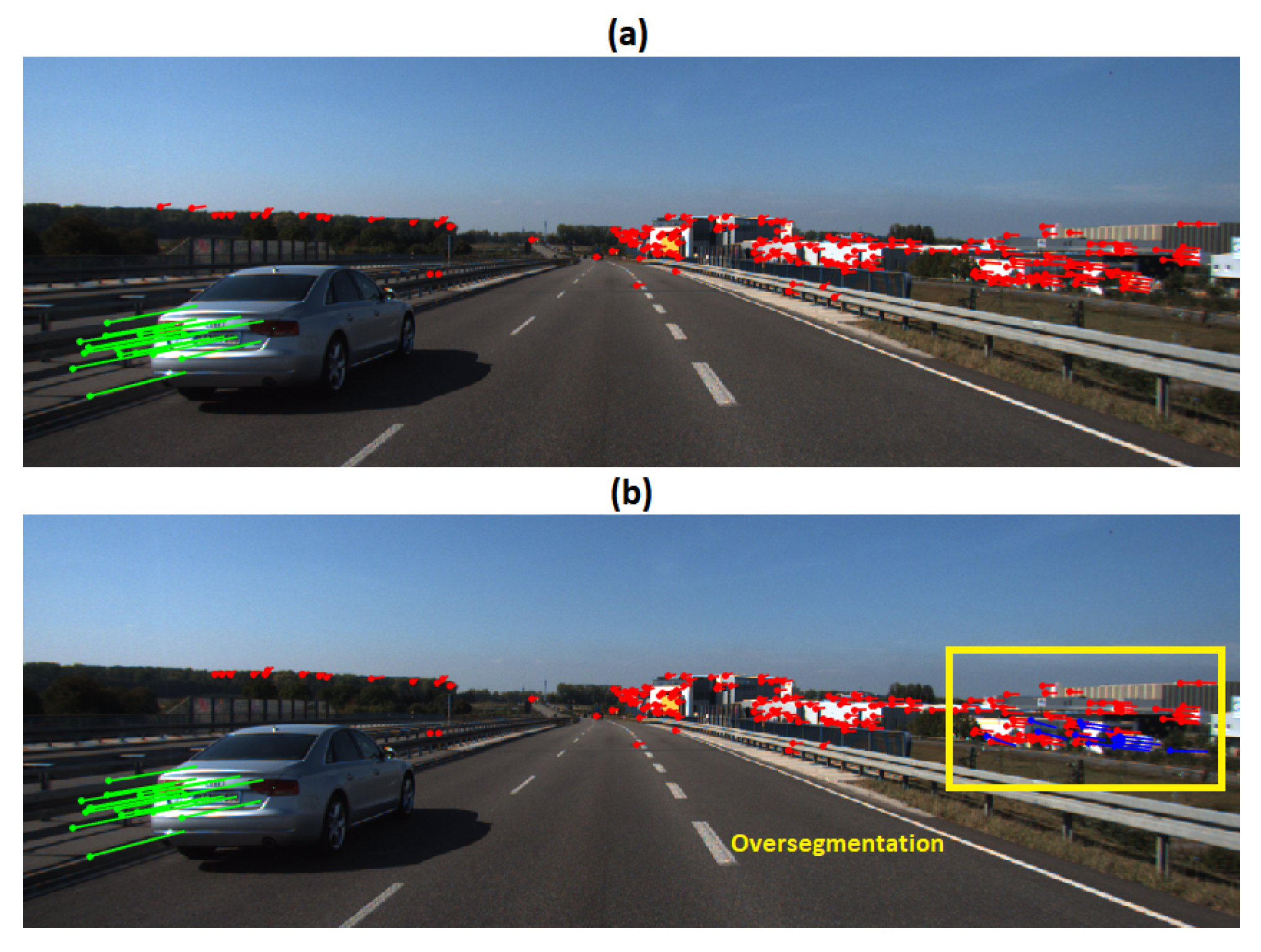
Figure 5 presents a scene composed of two simultaneous motions called Car2 (named Scene 3). The baseline method was parametrized considering 200 scene motion segmentation hypotheses by frame along the sequences. Thirty frames were processed using 26 sliding windows, each frame includes 490 feature points. The best precision and recall values were obtained with
pixels and
as reported in the
Table 4.
In
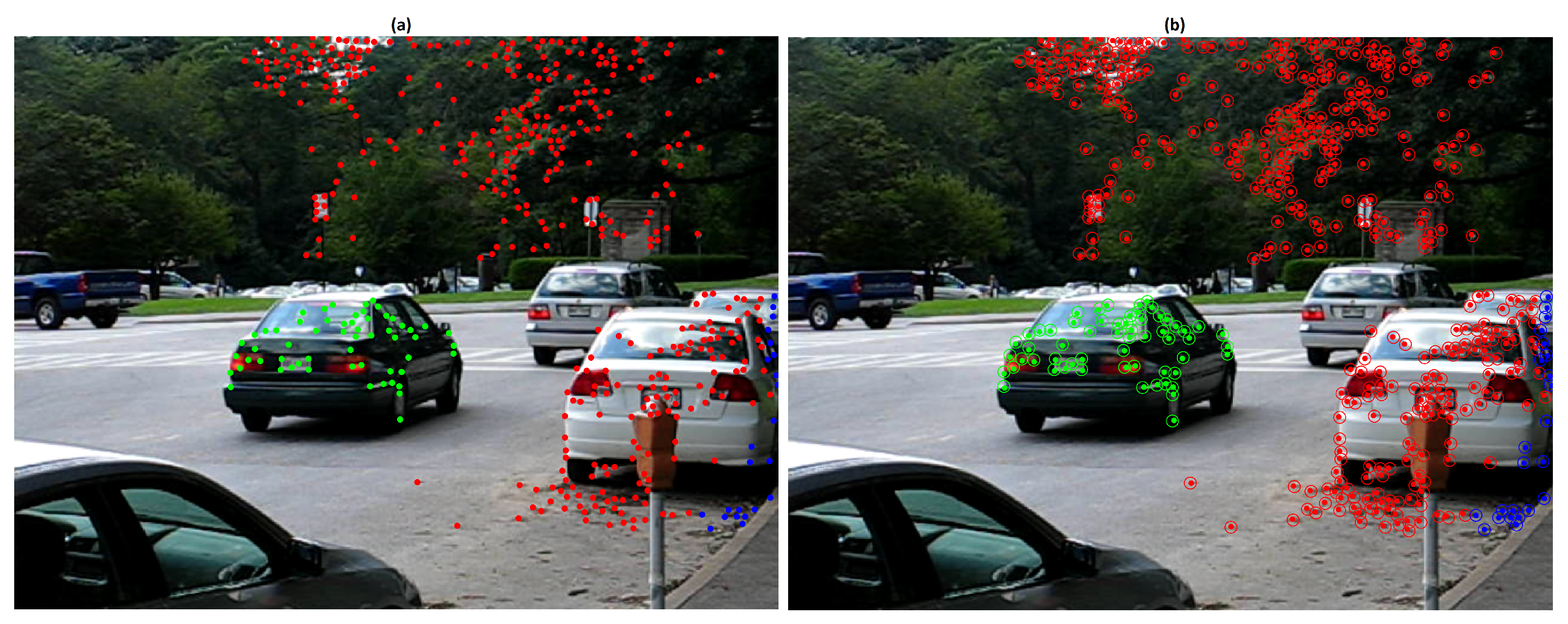
Figure 5, the segmentation and the reprojection error obtained with the baseline method in the first frame of the scene are shown. The moving object was segmented correctly, however, the dominant motion was over-segmented. A third group in blue was created with few feature points. The right image exposes the reprojection error in the first frame.
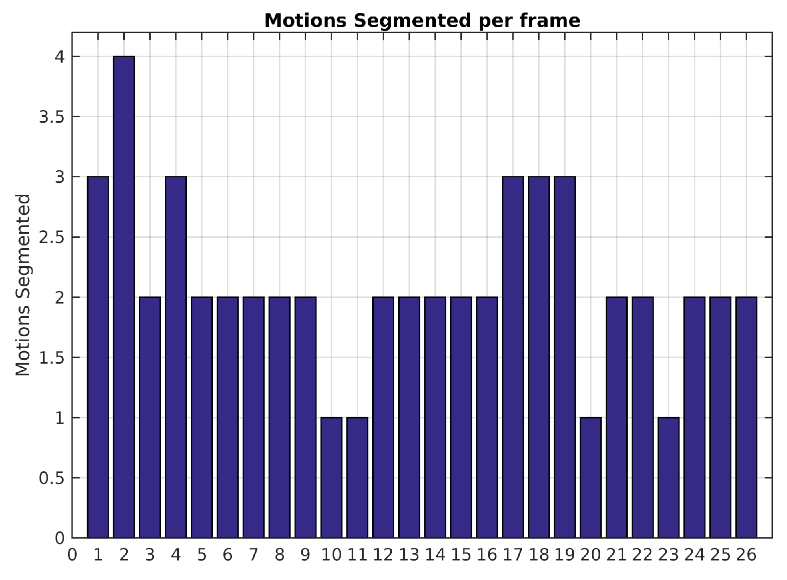
Figure 6 shows the number of segmented motions reported by the baseline method along the sequence. Since the scene is only composed of two independent motions, results with more than 2 are over-segmented and less than 2 are under-segmented. The low recall value of 0.66 (see
Table 4) is caused by the incorrect segmentation in the frames 10, 11, 20 and 23. This is probably due to the fact that the observed vehicle slows down. Decreasing the value of
may help to segment small inter-frame motions but can also lead to over-segmented scenes.
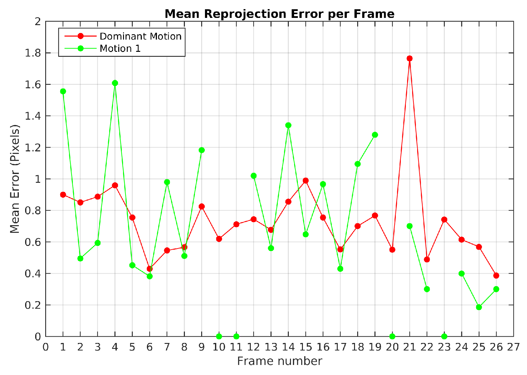
Figure 7 plots the mean reprojection error of the motions detected by the baseline method in Scene 3. In green dot-line, the moving object motion and in red dot-line the dominant motion (ego). Since the moving object was missed and its feature points were assigned to the dominant motion set in frames 10, 11, 20 and 23, no reprojection error was computed. The highest reprojection error was 1.9 pixels in frame 21 for the dominant motion and 1.6 pixels in the frame 4 for the moving object motion. Despite these reprojection errors, motions were segmented correctly.
The TbD-SfM was parametrized assuming an outlier ratio of 30% and thresholds values
pixels and
. Threshold values were selected following precision and recall scores computed for the first frame of Scene 3 and reported in
Table 5. A good feature points classification was obtained and no over-segmented areas were observed in the frame.
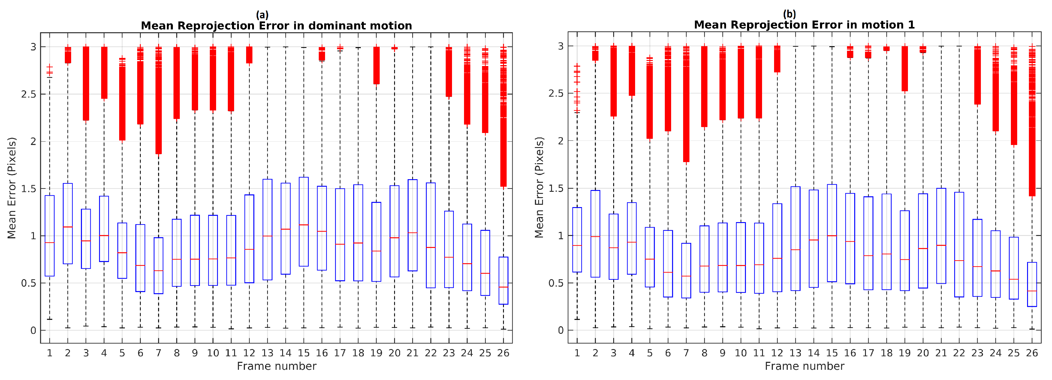
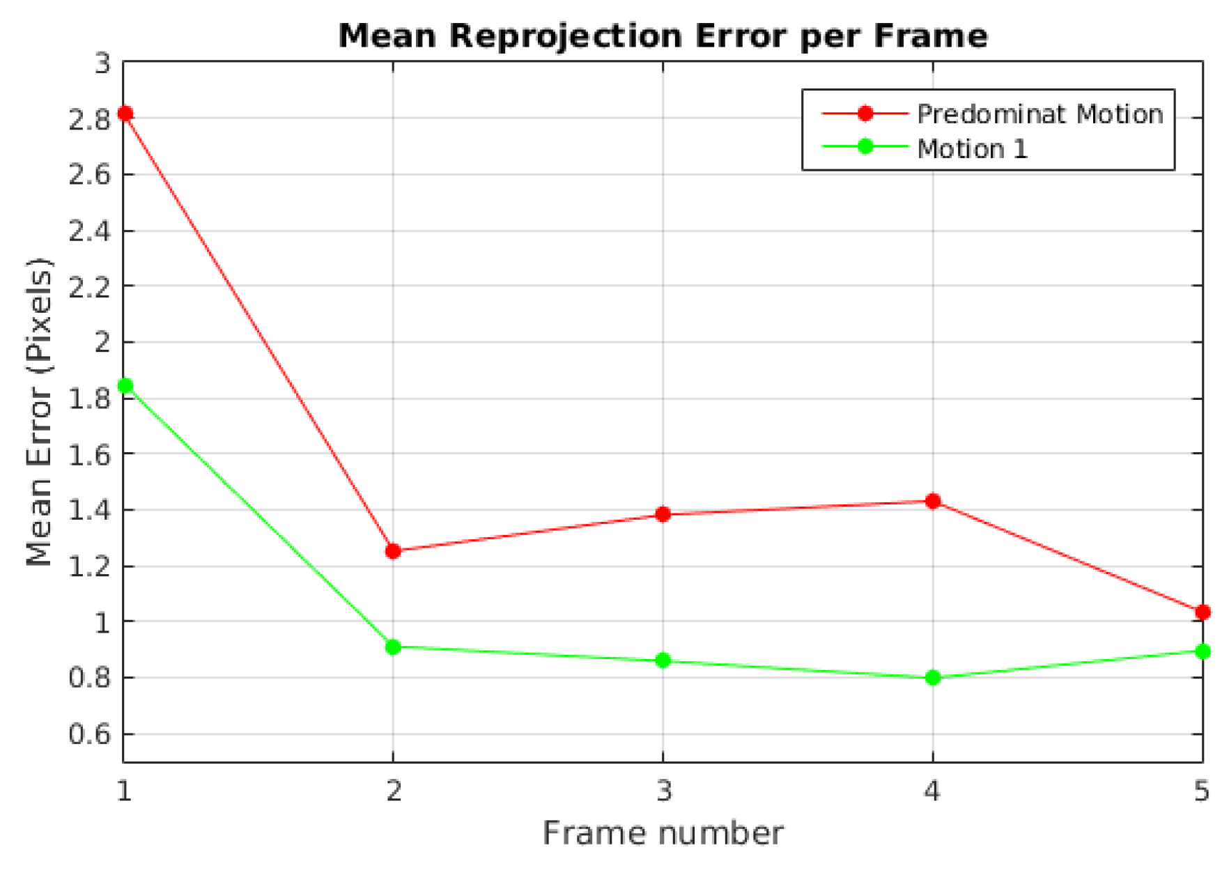
For the complete sequence Scene 3, the two motions were segmented correctly using TbD-SfM. The highest mean reprojection error was of 1.35 pixels for the dominant motion and 0.8 pixels for the moving object as shown in
Figure 8.
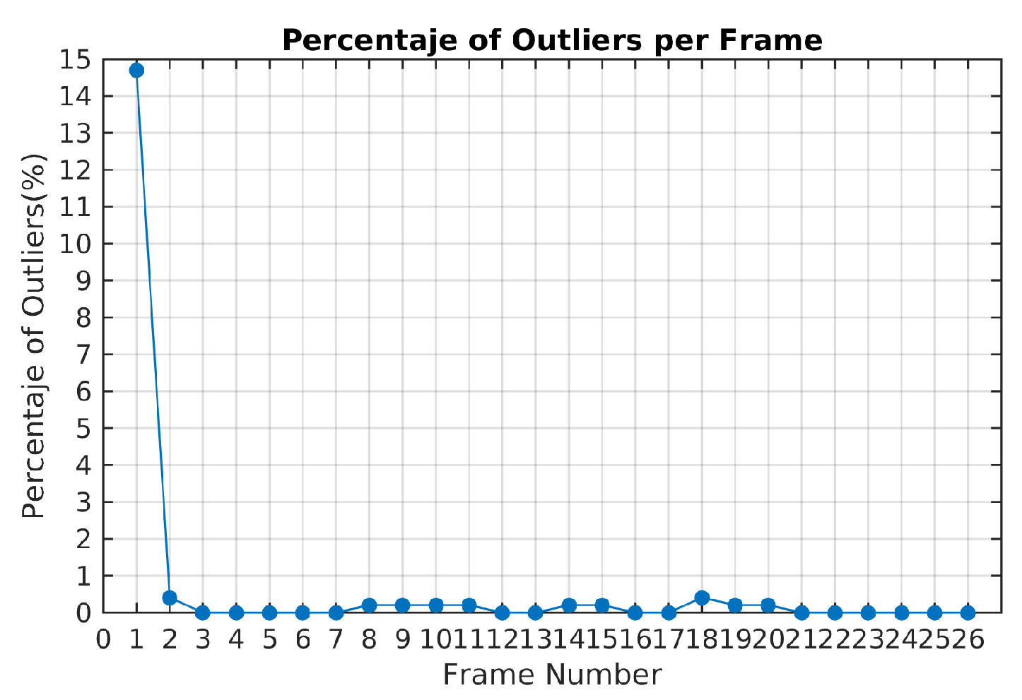
The ratio of outliers per frame is illustrated in
Figure 9. The highest value corresponds to the first frame estimation. In the next frames, the ratio of outliers with the TbD-SfM approach was less than 1%.
A Monte Carlo experiment was carried out in order to evaluate the repeatability and the stability of TbD-SfM results. To this end, scene segmentation was performed on 100 repetitions. The highest reprojection error was limited by the threshold
. The boxplot illustrates (see
Figure 10) that frames 13, 14, 15, 18, 21 and 22 used the range established in
. Others frames had the maximum boxplot value of the mean reprojection error results less than
threshold.
The highest percentage of outliers observed along Scene 3 is less than 2% as shown
Figure 11. At least 98% of feature points by frame were correctly classified and not rejected as outliers.
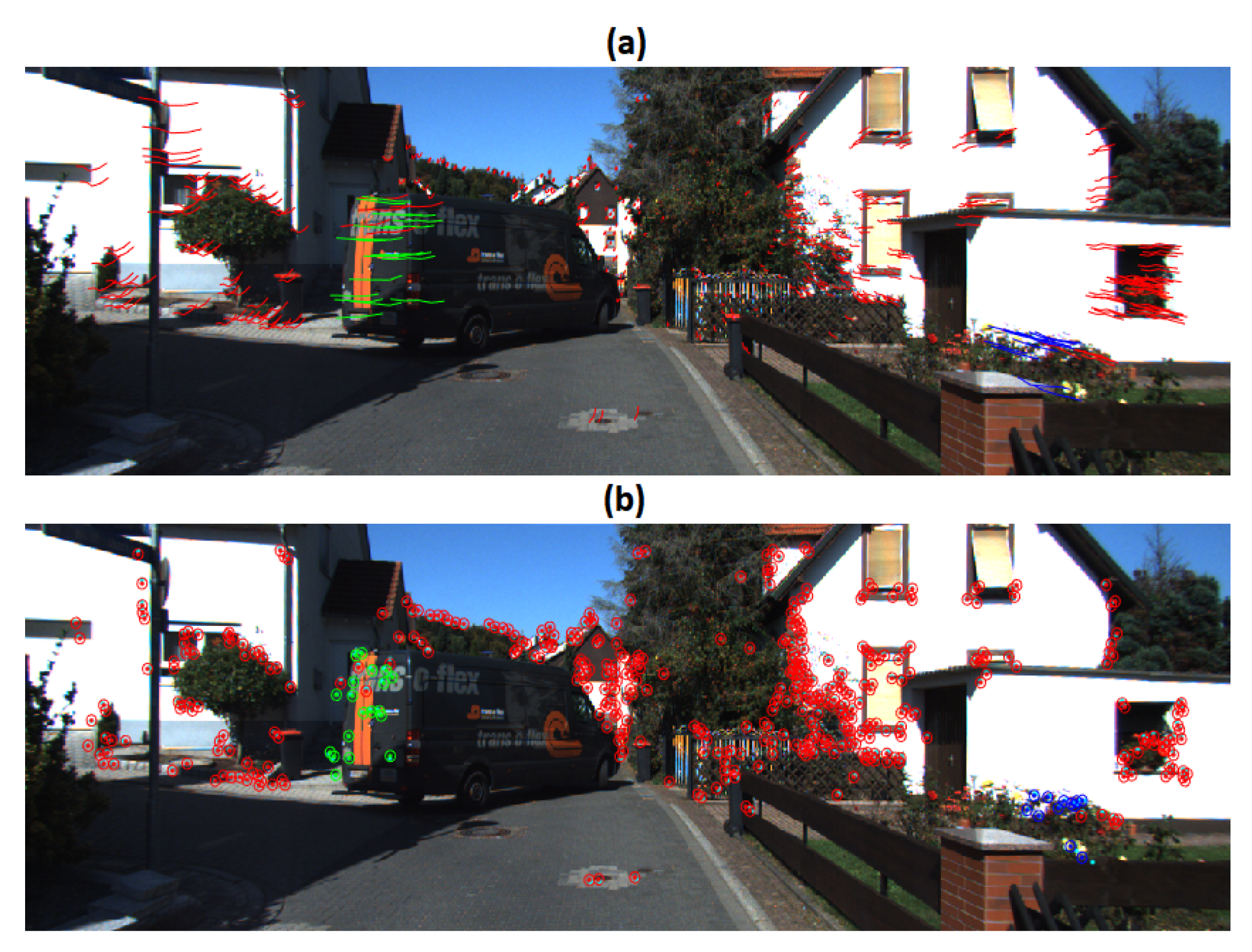
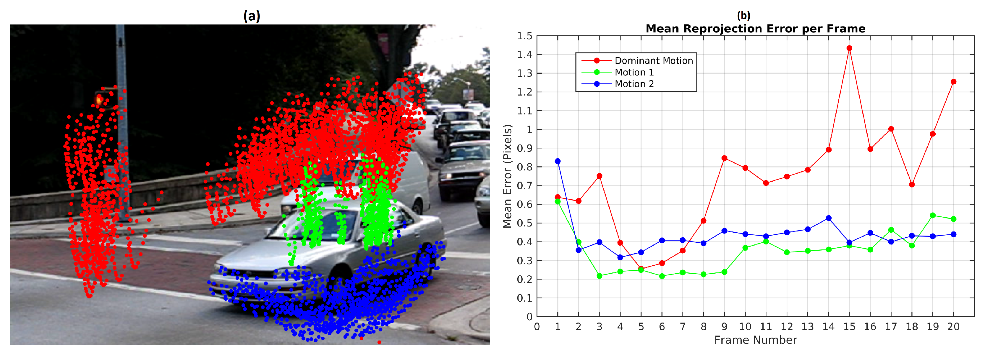
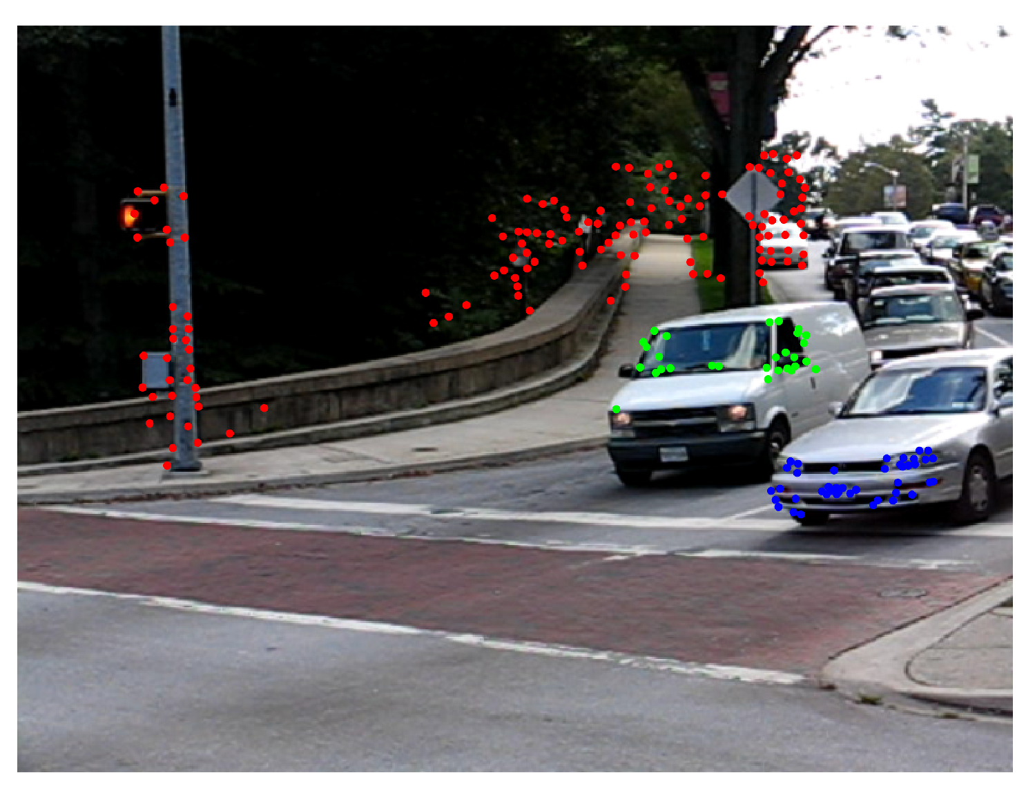
Figure 12 shows motion segmentation for the first frame of Hopkins 155 Car 9 sequence called Scene 4. The scene is composed of three simultaneous independent motions: the dominant motion (static objects in red) and two moving objects (green and blue). This sequence is a challenging use case since the observed objects moves at slow speed. Twenty four frames were processed with 220 feature points per frame. The baseline method was set to consider 300 scene motion segmentation hypotheses by frame. Results of the sequence are quantified in
Table 6. Reported results were obtained with threshold values
pixels and
pixels. The
Figure 12 illustrates the motion segmentation result for the first frame.
Despite the fact that precision and recall scores in
Table 6 are high, motion segmentation errors are still present along the sequence. That is the case for frames 4, 12 and from 14 to 20 where the baseline method over-segments motions and misses one of them in frame 8 (
Figure 13).
Figure 13b illustrates as an example the segmentation result of frame 12.
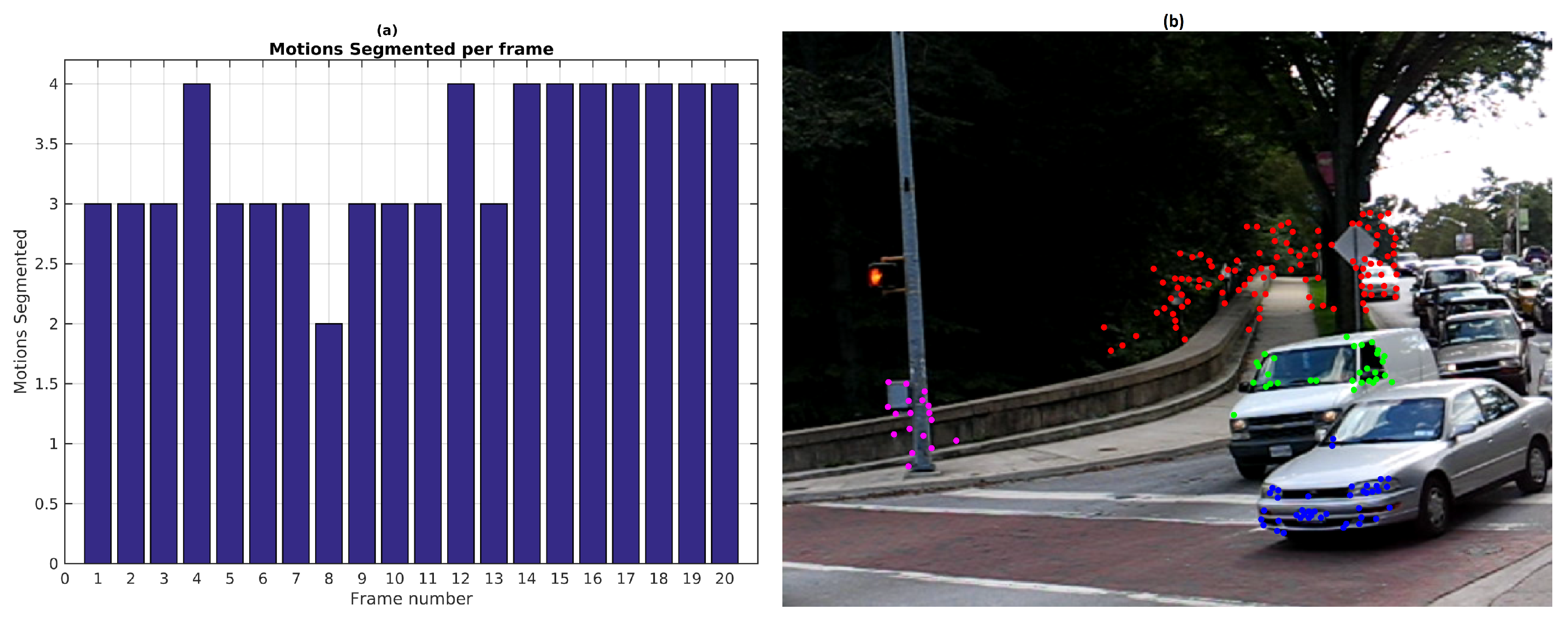
Figure 14 illustrates the mean reprojection error evolution in Scene 4, the highest value was obtained in the 13th frame for the 2nd observed motion with 1.2 pixels. The 8th frame shows that the 1st observed motion was not detected.
The TbD-SfM was tested with the same values
pixels and
and a RANSAC outlier ratio of 30%. The three motions were segmented correctly.
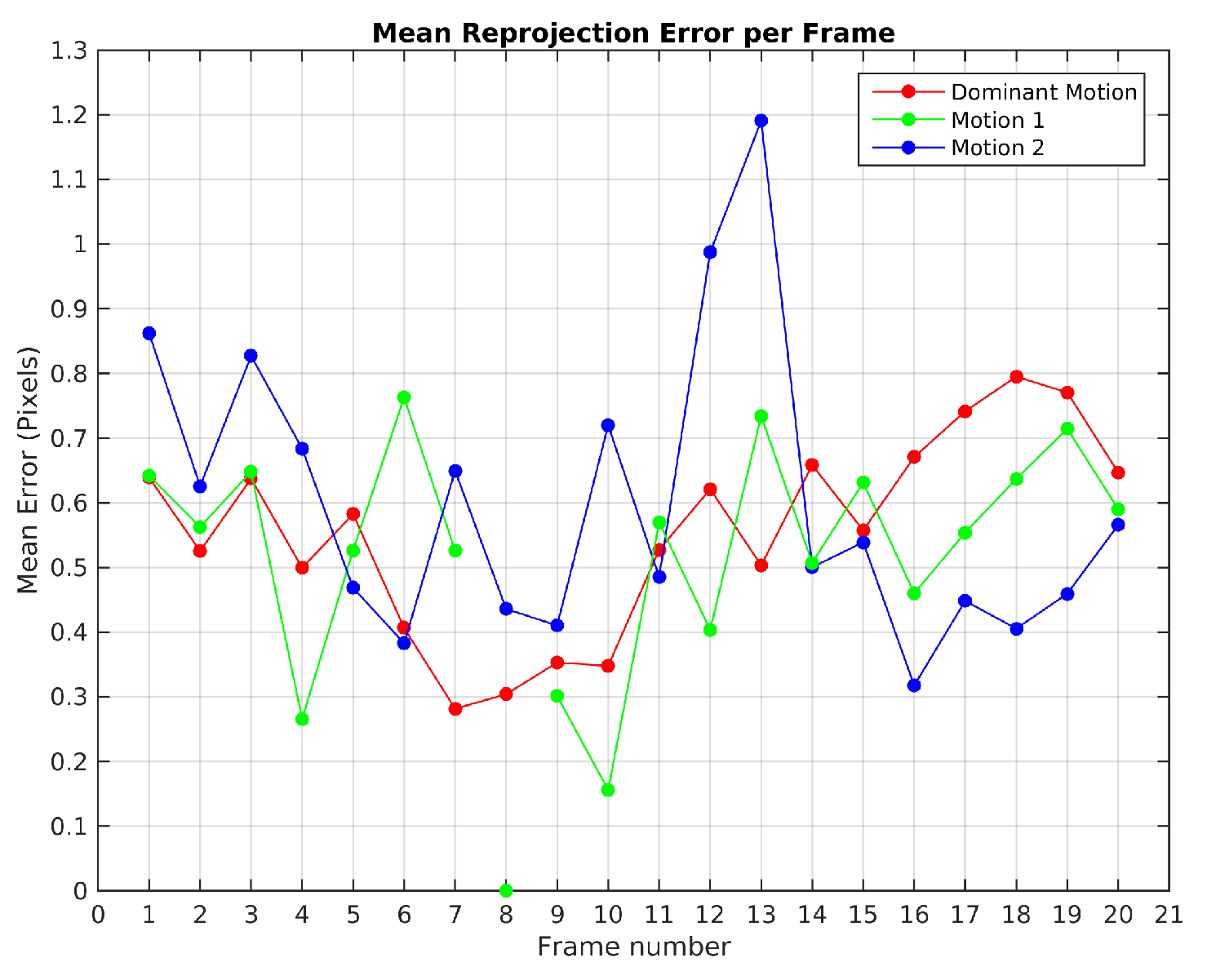
Figure 15b shows the mean reprojection error with a highest error of 1.45 pixels for the dominant motion. The highest reprojection error in the moving objects were less than 0.55 pixels.
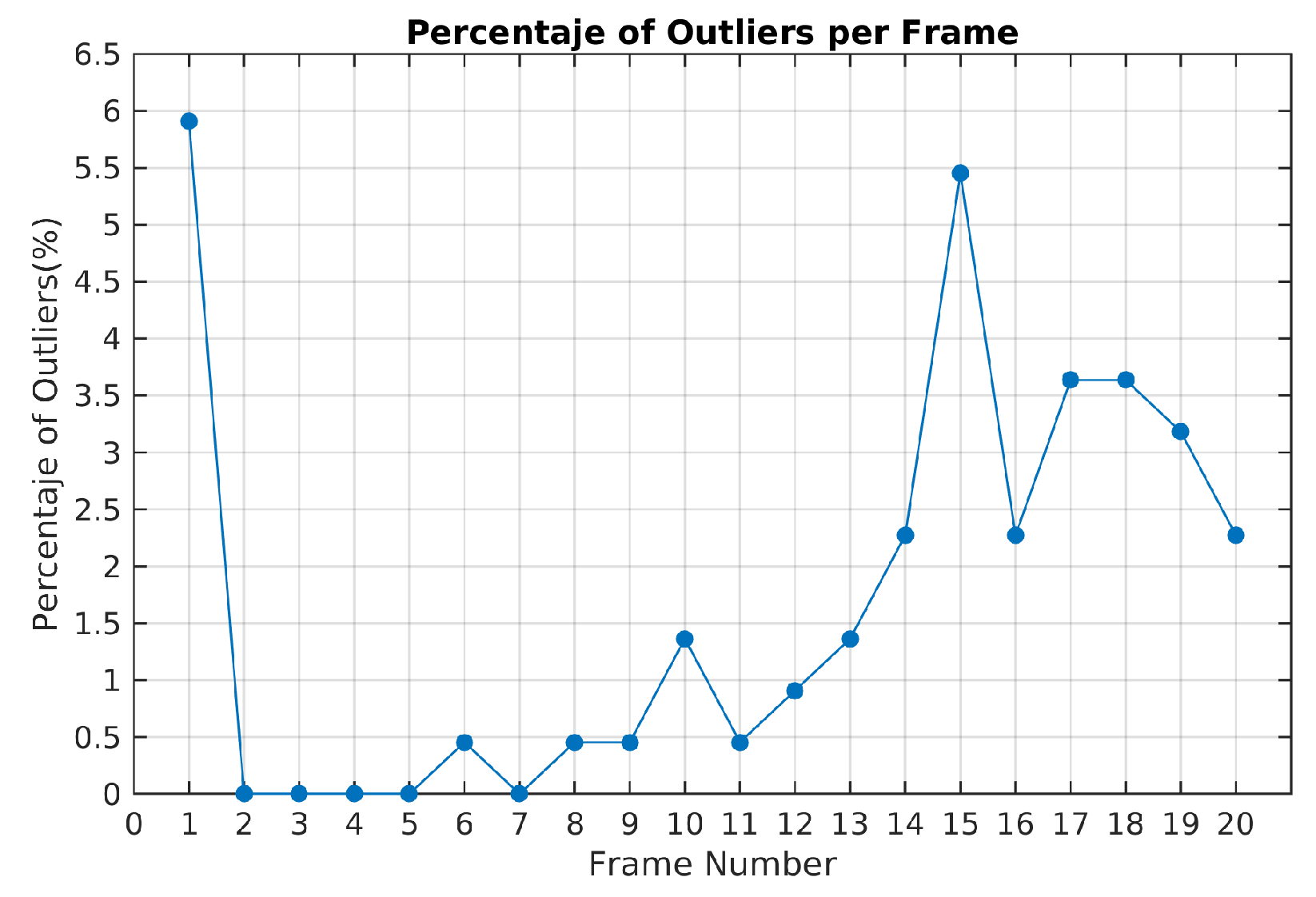
The highest percentage of outliers was obtained in frame 15 as illustrated in
Figure 16. In this frame, it was also obtained the highest reprojection error in the dominant motion. In this case, the selected hypotheses increases the reprojection error in the feature points and some of them were rejected. A high percentage of outliers are coming from the dominant motion even when the reprojection error is less than 1.5 pixels. The opposite situation was presented in the frames 2, 3, 4 and 5 where all the feature points were segmented correctly.
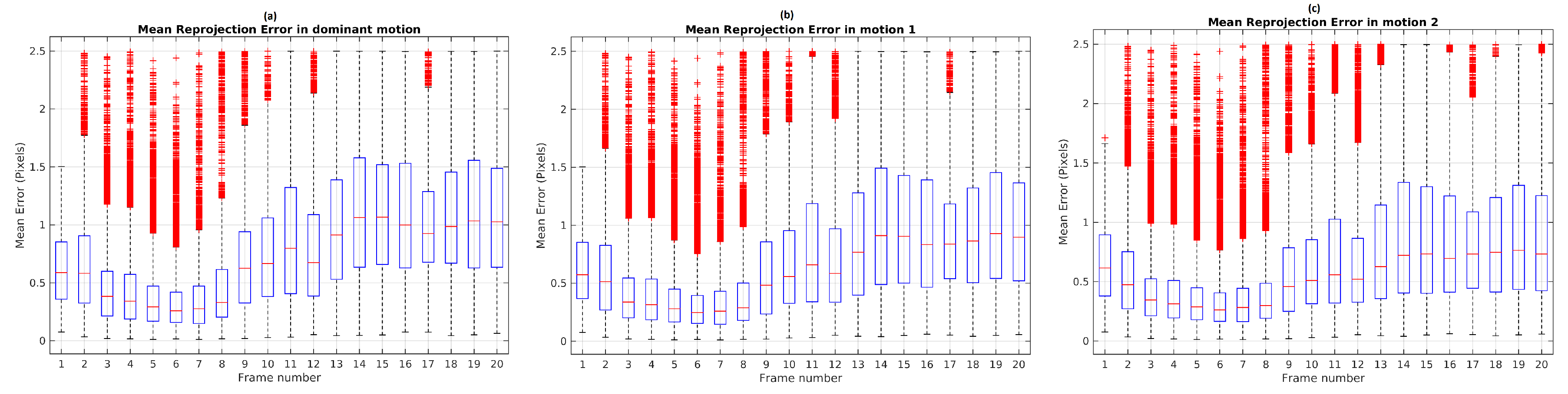
The results of the Monte Carlo experiment with TbD-SfM in Scene 9 are shown in
Figure 17. The highest reprojection error was limited by the threshold
. In a scene composed of three observed motions, the frame range from 3 to 8 shows that the maximum boxplot value for the mean reprojection error is less than 1 pixel. After frame 10, the upper whisker is greater because the moving objects are getting closer to the camera.
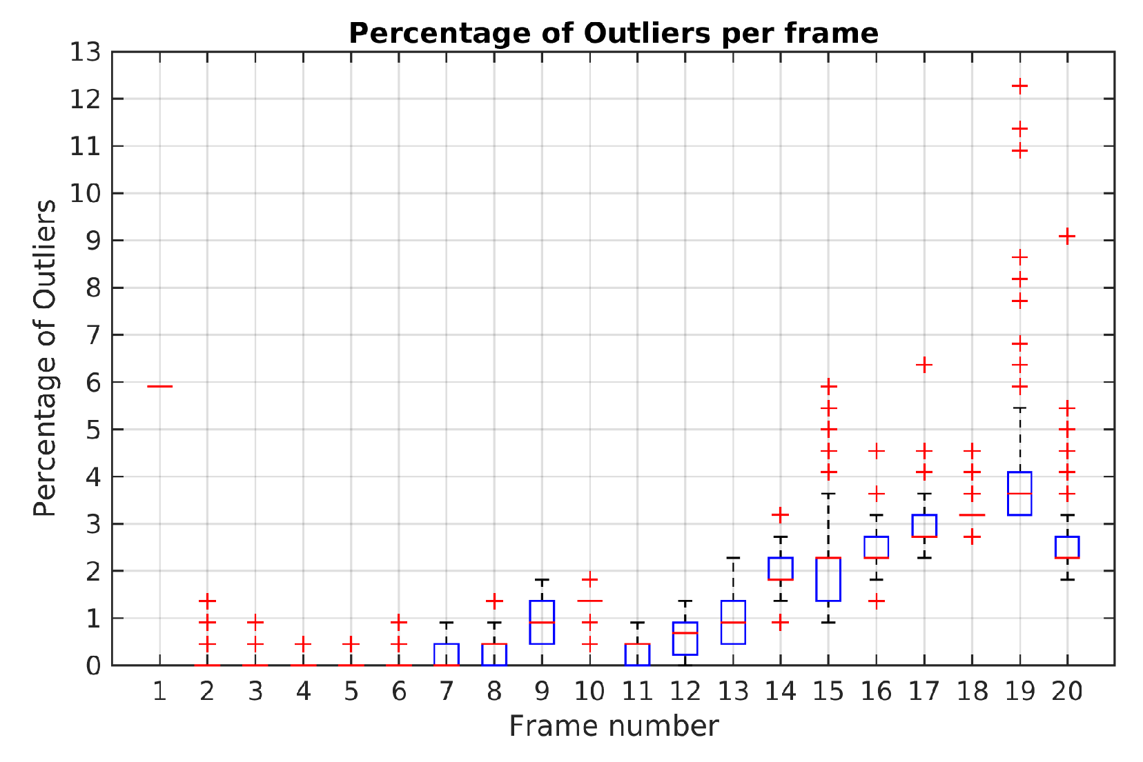
Figure 18 illustrates the boxplot results of Monte-Carlo experiment in Scene 4. It is noted that until frame 14 the maximum percentage of outliers obtained was 3.1%. In frame 19, it is shows a maximum boxplot value of 5.5% and the highest percentage of outliers with 12.2%. Except for this frame, the maximum boxplot value for the percentage of outliers is less than 4%.
Table 7 summarizes the evaluation results of the Monte Carlo experiments in Scene 3 and Scene 4 using TbD-SfM method. In Scene 3, TbD-SfM achieved a mean reprojeccion error of 1.25 pixel, a segmentation error of 0.01% and a mean outliers percentage of 0.8%. In Scene 4, it was obtained a mean reprojeccion error of 0.84 pixel, a segmentation error of 0.19% and a mean outliers percentage of 3.1%.
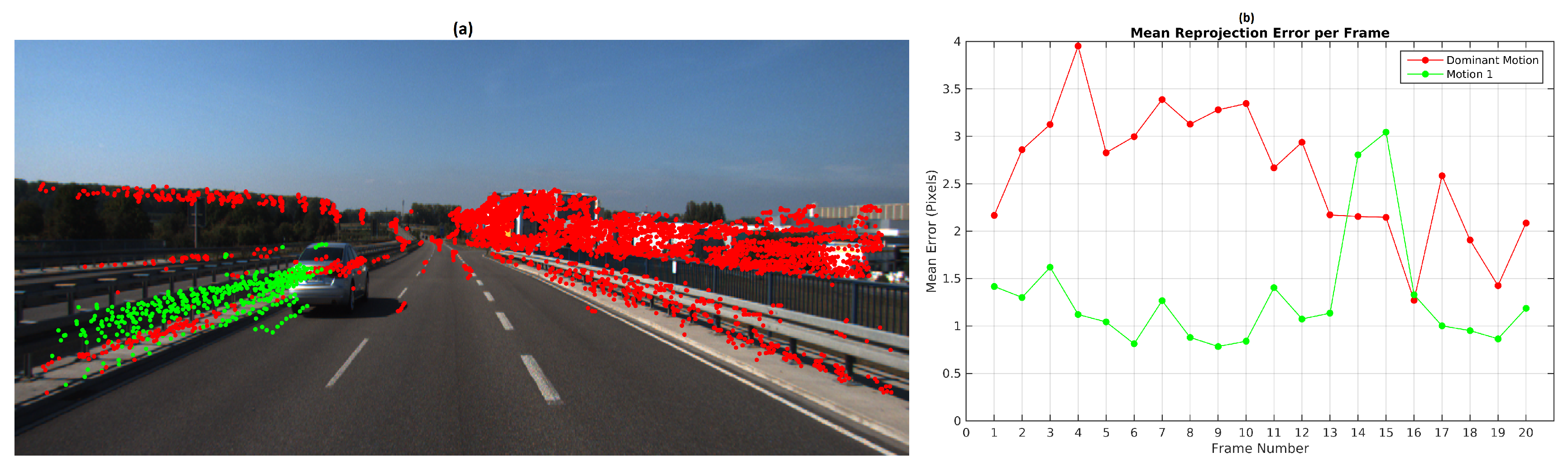
Scene 1 (
Figure 2) from KITTI dataset was processed with the baseline algorithm and TbD-SfM. A sequence of 20 frames with an average of 185 feature points by frame was processed. The baseline method was used to create 200 scene motion segmentation hypotheses by frame with the values
and
. The
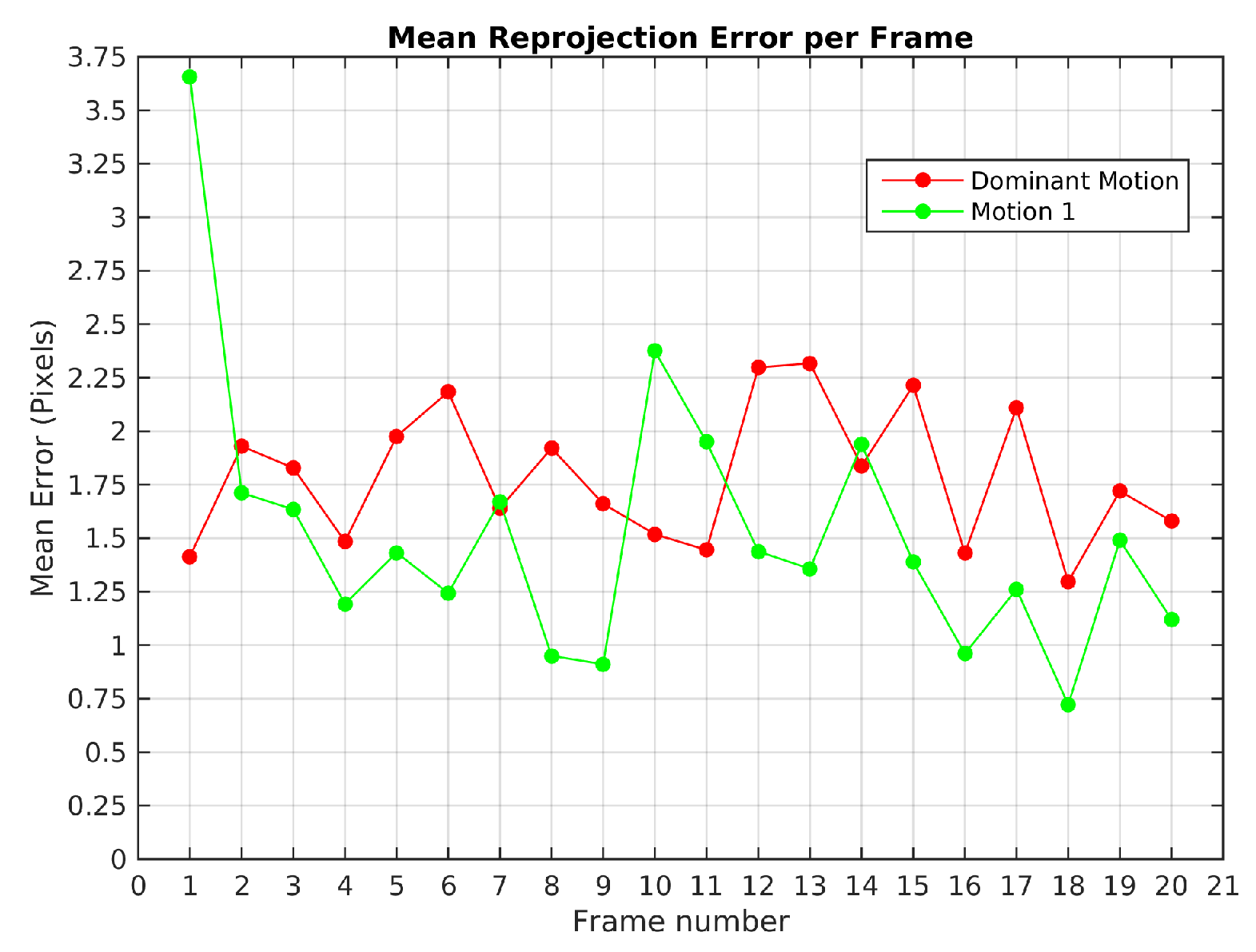
Figure 19 illustrates the mean error reprojection error for the two segmented motions, the highest value was 3.6 pixels for the moving object in the first frame.
TbD-SfM was set to assume an outliers ratio of 35%. The highest mean reprojection error was in the 4th frame of the dominant motion with 4 pixels as shown in
Figure 20b. One can notice that reprojection errors in KITTI dataset are higher than the ones achieved on Hopkins. Since Hopkins provides error-free feature tracking, reprojeccion errors are greatly improved. KITTI experiments shows the robustness of the proposed method to feature tracking errors and their impact in terms of the reprojeccion error.
The segmentation results along the sequence are presented in
Figure 20a. The feature points located in the side-view mirror of the vehicle were not segmented correctly. Since these points are observed in some frames outside of the predicted area, they were segmented in another group or classified as outliers. It was obtained a segmentation error of 1.4% along the sequence. The results are detailed in the
Table 8.
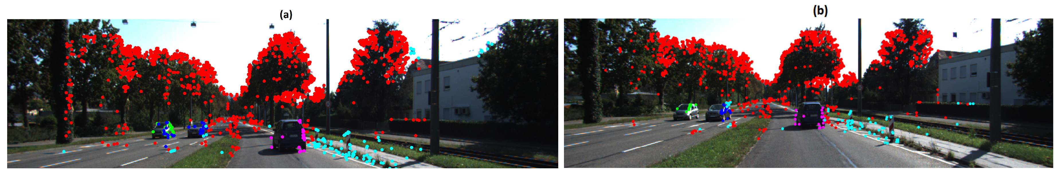
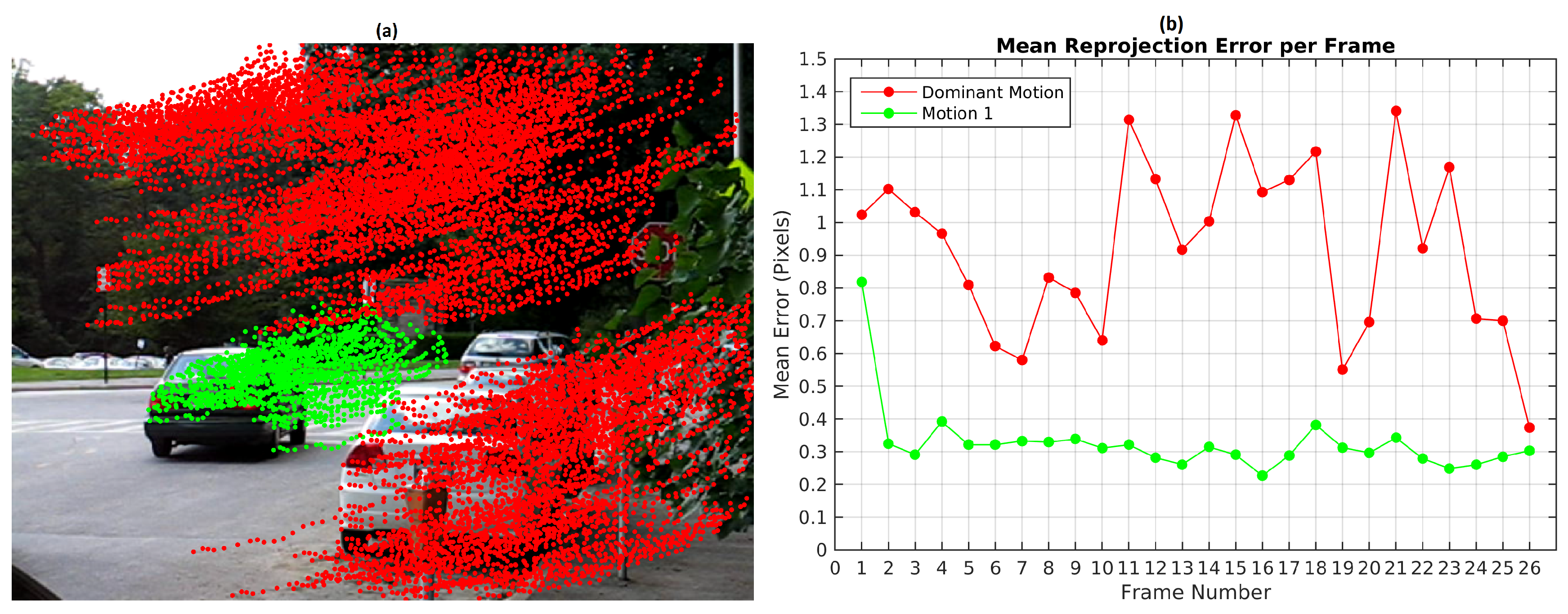
TbD-SfM efficiently addresses the scalability problem presented in the baseline method when the number of simultaneous motions increases. In the Scene 5, the scalability of TbD-SfM was tested in a scenario with 4 simultaneous motions as shown in
Figure 21. There are two moving objects approaching to camera with different speeds and a third one moving along the moving camera. 8 frames were processed with 4 sliding windows, an average of 1450 feature points are observed by frame. The first frame segmentation was obtained with the baseline method considering 400 scene motion segmentation hypotheses with the parameters of
pixels and
. In the first frame, some segmentation errors were observed: some feature points of the moving object 1 (green) were assigned to the moving object 2 (blue). However, the TbD-SfM procedure allowed to correct these errors and enhanced the segmentation as shown the frame 4. The outliers feature points are shown in cyan color.
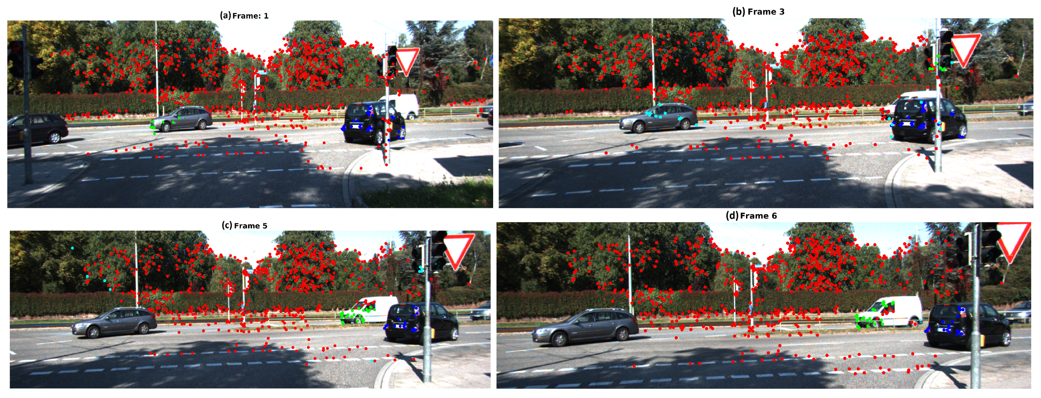
In Scene 6, TbD-SfM was implemented in a sequence under particular characteristics. The moving camera is turning right, objects enter or leave the scene and some of them are partially occluded. This scene allows to test the detection and segmentation of new moving objects. It were processed 6 frames with an average of 670 feature points per frame. The moving objects are represented by the green and blue feature points. The parameter values employed in this sequence were
pixels,
and it was assumed an outliers ratio of 45%.
Figure 22 illustrates the results obtained by frame with TbD-SfM approach. In the first frame, it was detected 3 simultaneous motions. The green moving object has a partial occlusion by the ego-motion feature points located over the traffic light post. In the third frame, a small group of feature points was segmented as other moving object over the traffic light post, however, this group is not detected in the next frames. The outliers feature points are represented in cyan, this points over the gray car were not associated because they do not meet the reprojection error criterion
. Some feature points of a new object(white car) were segmented with the dominant motion. In the 5th frame, the white car was detected as new moving object for first time and some segmentation errors. In the 6th frame the new moving object is detected with a better segmentation. The results evaluated are reported in the
Table 8.
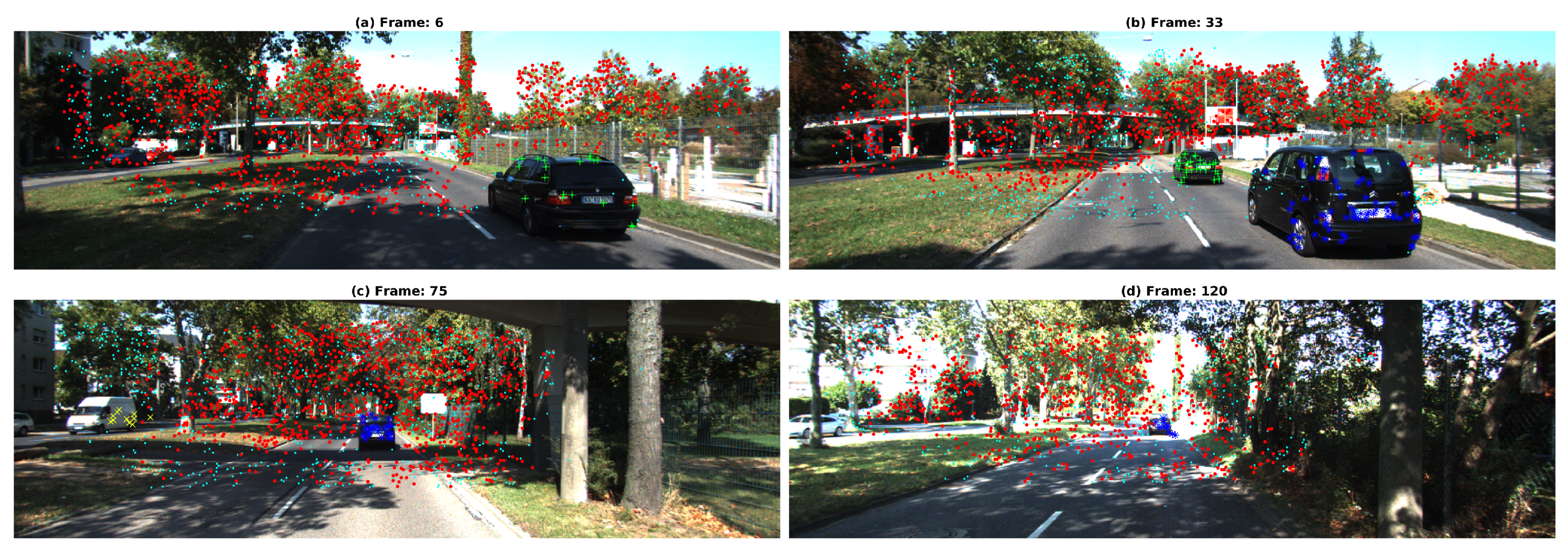
It is worth to mention that performances and execution time of the TbD-SfM were also evaluated on a long sequence context. In the Scene 7, 130 frames were processed involving a moving ego-camera, two cars passing from back to the front and a third car approaching. As an example, the
Figure 23a shows the 6th frame where the first moving object was segmented. A second car was then detected and segmented as shown the
Figure 23b.
Figure 23c presents the second car marked in blue is occluding the first detected moving object. At the left side, a van approaching to the ego-camera that was segmented and marked in yellow. Finally, the
Figure 23d illustrates 120th frame where the object was segmented while it moves away. Performance results are reported in the
Table 8.
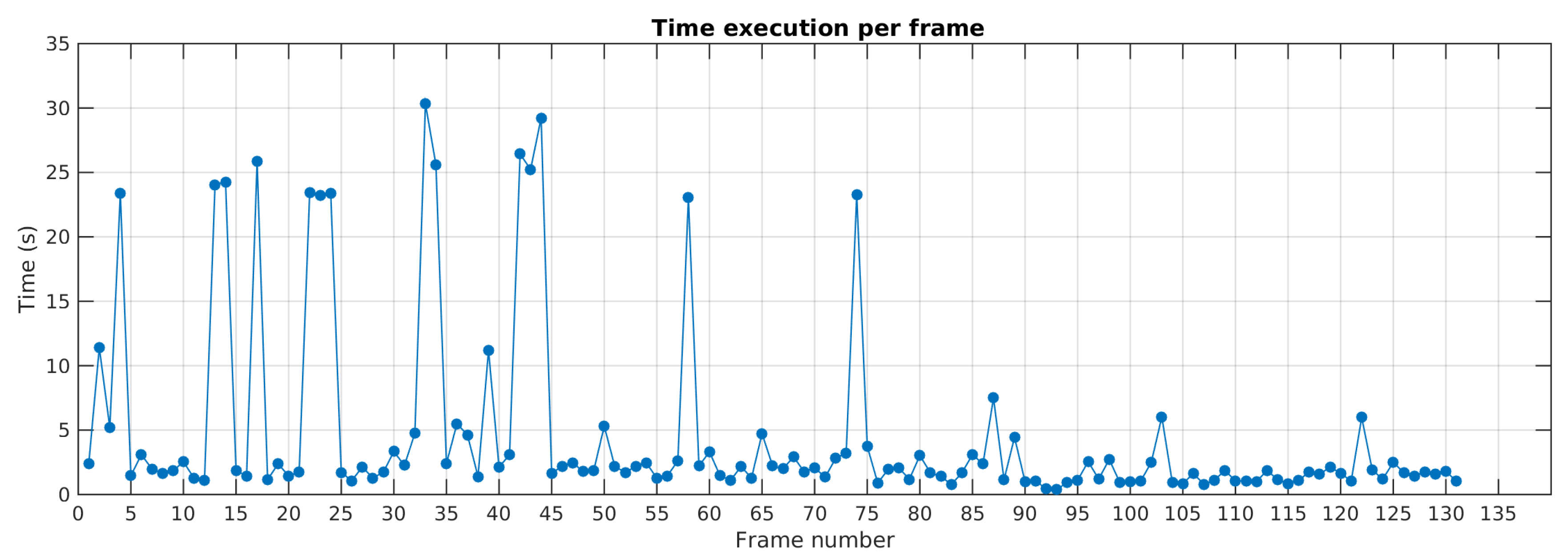
The
Figure 24 details the execution time per frame along the sequence in Scene 7. The results show that before the 50th frame, run time is higher due to a greater amount of dynamic feature points. After, run time decreases. It is worth noting that the detection of new motions requires more processing time due to feature resampling task. That can be observed by run time peaks in frames 14, 22, 34, 44, 57, 74. This processing time can be greatly enhanced by parallelizing or pipelining feature resampling and motion tracking threads.
TbD-SfM was tested in car sequences of Hopkins dataset for allowing comparison with other methods. The dataset has 8 scenes with two simultaneous motions and 3 scenes with three simultaneous motions. The algorithm was run once by sequence and the results reported in the
Table 9. The highest mean reprojection error was of 1.25 pixels for Car2 sequence and the highest segmentation error and outliers percentage were 0.2% and 6.1%, respectively, for the Truck2 sequence.
Table 10 shows a benchmark comparison of the car sequences results using TbD-SfM (
Table 9) and other state-of-the-art methods [
38,
39]. The results presented in the
Table 10 shows that TbD-SfM achieves a lower segmentation error in scenes with two and three simultaneous motions in comparison to methods presented in [
18,
20,
21,
22,
24,
26,
27,
28,
29,
30,
31,
32]. TbD-SfM obtains a segmentation error of 0.07% for sequences involving three simultaneous motions. This error is higher in comparison to HSIT [
23] that reaches a perfect segmentation. In contrast, the segmentation error in two simultaneous motions sequences of TbD-SfM is 0.02% compared to 1.65% of HSIT that is 82 times lower. TbD-SfM has similar performance in comparison with the DCT [
19]. The DCT segmentation error was 0.05% considering all the sequences of the dataset, while TbD-SfM segmentation error was lower in datasets with two motions by a difference of 0.03% and higher by 0.02% for three motions dataset. Comparing TbD-SfM to the baseline method, the segmentation error is higher by a difference of 0.02% in sequences with two simultaneous motions and lower by 0.04% in datasets with three simultaneous motions. In particular, TbD-SfM have obtained a greater number of feature points correctly segmented in comparison with the baseline method as shown the percentage of outliers in the
Table 9. It is worth noting TbD-SfM achieves a denser feature segmentation than the baseline approach. That is because the baseline approach performs an optimization step intended to enhance motion segmentation by rejecting feature points with a high reprojection error. This procedure can certainly improve motion estimates but it also reduces the number of feature points that represent a motion. Objects with few features may be easily lost or missed detected.
The results show that our algorithm outperforms the RANSAC formulation proposed in [
31]. The reprojection error obtained with TbD-SfM algorithm can be reduced with an optimization method over the RANSAC formulation as described in [
40,
41].
The reported experiments were obtained thanks to Matlab implementations on a laptop with processor i-7 2.6 GHz and 16 GB-RAM. The average running time of the baseline method for two, three and four simultaneous motions were 85.2 s, 259 s and 6360 s. For TbD-SfM method execution time decreases in average to 3.5 s, 3.9 s and 78.3 s for two, three and four simultaneous motions, respectively.


