Abstract
Security risks and economic losses of civil aviation caused by Foreign Object Debris (FOD) have increased rapidly. Synthetic Aperture Radars (SARs) with high resolutions potentially have the capability to detect FODs on the runways, but the target echo is hard to be distinguished from strong clutter. This paper proposes a clutter-analysis-based Space-time Adaptive Processing (STAP) method in order to obtain effective clutter suppression and moving FOD indication, under inhomogeneous clutter background. Specifically, we first divide the radar coverage into equal scattering cells in the rectangular coordinates system rather than the polar ones. We then measure normalized RCSs within the X-band and employ the acquired results to modify the parameters of traditional models. Finally, we describe the clutter expressions as responses of the scattering cells in space and time domain to obtain the theoretical clutter covariance. Experimental results at 10 GHz show that FODs with a reflection higher than −30 dBsm can be effectively detected by a Linear Constraint Minimum Variance (LCMV) filter in azimuth when the noise is −60 dBm. It is also validated to indicate a −40 dBsm target in Doppler. Our approach can obtain effective clutter suppression 60dB deeper than the training-sample-coupled STAP under the same conditions.
1. Introduction
The background of this research is the multi-death crash of Concorde Air France in 2000, which was caused by a piece of debris on the taxiway and evinces the need to detect Foreign Object Debris (FOD) on runways. FODs may lacerate aircraft tires or wear engines [1] during taking off and landing. According to statistics from Insight SRIT, the authoritative analysis company in UK, over 66% of airport emergencies are related to FOD [2]. It has become the second most common threat to aviation security after bird hit.
The International Civil Aviation Organization stipulates explicitly that at least four-time inspections per day must be ensured to the runway. While manual inspection can only guarantee safety for 1% of the flights, the automated FOD detection systems could provide nearly 100% effective inspections for all flights [3].
In existing systems [4,5,6,7], the radar and Electro-Optical (EO) hybrid devices are most commonly utilized. But EO sensors will be greatly weakened in inclement weathers [8,9]. In comparison, radars can provide all-time and all-weather inspection to runways [10]. Wide band millimeter-wave radars have high enough resolutions to detect small pieces of metal, stones, concrete or even plastics on runways. For instance, COBRBA-220 [11], the ultra-wide-band system, could reach a resolution of 1.8 cm. The 77 GHz FOD detection radar [12] developed under the cooperation between Japan and France showed signal attenuation less than 0.18 dB as well as high sensitivity to −20 dBsm objects. In recent years, performances of some other radars working around 70 GHz [13], 76.5 GHz [14], 78 GHz [15,16], 96 GHz [17], even 110 GHz [18] have been successively validated by test data in controlled conditions (e.g., wave form, polarization, and antenna gain).
Although stationary FOD detections have been well developed by Constant False Alarm Rate (CFAR) algorithms [19,20,21,22], the radar-based FOD surveillance is still challenged by finding debris in different motion states (e.g., rolling small screws, wind-driven plastic bags [23,24] and invading wildlife [1] (p. 1), especially in clutter conditions [3].
Space-time Adaptive Processing (STAP) [25,26] has been maturely utilized in Synthetic Aperture Radar (SAR) to suppress ground clutter and indicate motive targets [27]. The same technique can potentially be utilized to design space-time filters to detect motive FOD in strong clutter, if exact clutter covariance estimation is obtained. STAP requires that the number of training samples [28] must have more than double Degrees of Freedom (DOFs) and be Independent Identically Distributed (IID) with the detected samples. However, these requirements are rarely satisfied in practice, which makes the STAP performance limited [29].
A series of methods have been proposed to release the IID constraint, and thus to accelerate computation and convergence. The most representative and widely used are the reduced-dimension and the reduced-rank STAPs [30,31,32], which operate on the basis of matrix transformations. The Sparse-Recovery (SR) STAP technique [33,34] has attracted great attention because it can reduce computation significantly in the case of insufficient training samples by making utilization of clutter sparsity in the space-time plane. By employing environment knowledge, Knowledge Aided- (KA-) STAPs are proposed with significant superiority, prominent value, and wide prospect to radar intellectualization. By utilizing prior information in algorithms directly, Bayesian filtering [35,36] and data pre-whitening STAPs [37,38] are investigated but the performance is influenced by the mismatch between prior knowledge and time-varying environment. Some other ideas have concerned environment sensing for intelligent sample selection [39,40] to analyze rather than estimate the clutter covariance by samples. But these STAPs demand exact backscattering coefficients and high resolution cells, with the support of real scene topography [41,42], digital elevation model data [43], hyper-spectral remote sensing images [44] and so on.
Based on the above analysis, we propose a clutter-analysis-based STAP for motive FOD detection in a familiar environment, which decouple from IID training samples to estimate clutter covariance. The prior knowledge could be easily obtained from the SAR observations, the high-resolution visible spectrum images, or the airport construction drawings [45] (pp. 4–7).
The rest of this paper is organized as follows: in Section 2, the radar coverage is divided into scattering cells based on the geometric model in xOy coordinates. In Section 3, the space-time clutter is deduced and addressed according to the parameter-modified scattering model. Section 4 concerns the filter design in the space-time domain. Experiments and discussions are overviewed in Section 5 that support the conclusions drawn in Section 6.
2. Scattering Cells
A novel scattering cell division method is introduced in this section as the foundation of clutter analysis. The geometric model of an airport is constructed at first to determine the radar covering area. Note that the polar coordinates are not applicable in this case. Therefore, we divide the scene into scattering cells in xOy coordinates for exact backscattering coefficients.
2.1. Geometric Model of Scene
Federal Aviation Administration has regulated FOD detection systems referring to installation, operation, maintenance, and renewal. Most equipment should be operated at a distance of greater than 50 m away from the runway and taxiway [41] and with a height of less than the safety limit (usually two meters) [41,45]. Below is the model depicting the geometrical relationships between the SAR and the scene.
As depicted in Figure 1a, the rectangular coordinates are better suited to the straight runway, where the origin is at the location of the platform and x axis is parallel to the runway. The side looking SAR, equipped with a Uniform Linear Array (ULA), is deployed on a platform L1 away from the L2-width runway and travels at a velocity of νplat towards the positive direction of the x axis. Note that the maximum radar range is much larger than the platform height h, which causes a very small grazing angle ψ.
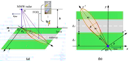
Figure 1.
(a) Geometrical model of foreign object debris (FOD) detection; (b) The vertical view of (a).
To simplify the analysis, we suppose that the radiation energy is concentrated within the main beam whose width is θB in azimuth and α in elevation. The orange area in Figure 1b highlights the area covered by the SAR beam. It could be divided into two semi-ellipses sharing the same short axis b, but they have different long axes denoted by a1 and a2. With the beam scanning, the coordinates could be transformed from xOy to x’Oy’ by θ between the beam and x axis:
The center (x0’, 0) is expressed as following:
a1, a2, b and x0’ are given in Equation (3).
where ψ is extremely narrow, which makes the approximate equality relations hold. Combining all of the above, Equation (2) is rewritten as
Equation (4) defines the area where clutter is generated, acting as the foundation of the following analysis. Without loss of generality, we focus on to analyze for more simple expressions.
2.2. Scattering Cell Dividing
Traditional STAPs perform well only in a homogeneous clutter background [44,46] and are usually investigated in polar coordinates. However, various terrains sharing the same range may result in different distributed clutter in airports. In this case, clutter covariance estimation by training samples will be not reliable.
Ground clutter is reflected by the statistical echoes of resolution cells, thus the cell area and backscattering coefficients are both required to calculate the RCS. The common range-azimuth dividing is depicted in Figure 2. The resolutions represented by and can be obtained according to the parameters of the transmitting wave. But those cells at the border between different scattering surfaces, such as runways and lawns, are hard to provide exact backscattering coefficients for clutter analysis. Therefore, we consider discussing the xOy system by dividing the radar covering area into several equal grids, which is expected to be more applicable to the straight runways.
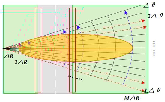
Figure 2.
Dividing the scene into resolution cells in polar system.
As is shown in Figure 3, we assume the beam exists in the dashed square. We divide the radar coverage into M equal stripes. The width of each stripe is . Each stripe contains 2L grids sized . Thus, every stripe is in length. We define the grid centers as , where . Notice that the cell area is independent of and . These grids are defined as the clutter scattering cells in this paper. We consider that each cell is isotropic where the backscatter coefficient keeps constant.
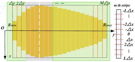
Figure 3.
Dividing the radar coverage into several grids sized .
3. Ground Clutter Deduction
According to the electromagnetic scattering theory, the ground clutter can be reasonably modeled by considering all scattering cells even in inhomogeneous clutter environments. In this section, first the classical Kulemin model is modified for low-grazing backscatter coefficients by the measured normalized RCS data in X-band and then the space-time coupled clutter is further deduced and investigated specifically for analysis and synthesis purposes.
3.1. Test-based Kulemin Model
At extremely narrow grazing angles (less than 5 degrees), the backscattering coefficient (RCS per unit area) acquirement is a problem in practical cases since the ground-clutter echo is hardly collected by the antennas. A series of empirical models covering almost 0–90 degrees are presented to depict the clutter statistics characteristic. Among them, the Kulemin model shows applicability at 3–100 GHz and low grazing angles less than 30 degrees, containing only three parameters determined by averaging the experiment data under several surface conditions (including humidity, roughness and vegetation types) [47] (pp. 17–20). Thus, it is usually preferred for simple expression and wide range applications to achieve backscattering coefficients of the concrete runways and surrounding lawns as a preliminary clutter estimation. The model is given in detail as [41]
where the carrier frequency and the grazing angle are evaluated in GHz and degree respectively. However, the echo is too small to be statistically significant when is very close to zero, which is seldom taken into consideration. Obtained by generalization of different cases, to are chosen according to Table 1:

Table 1.
Parameter choices of Kulemin model [41,47].
Based on the experimental evidence, this model could describe the statistical trend of ideally but hardly complete accurate clutter modeling in certain conditions.
Even with a lack of measuring data at small grazing, test results in higher elevation cases have the potential to modify to by LS fitting (the derivation and calculation details are given in Appendix A), so as to approach the low-grazing situations. More specifically, the low-grazing could be directly calculated when is put into the modified model.
The measuring data have been gathered in our labs. Figure 4a shows the experimental set-up. The typical ground samples (see Figure 4b,c), located on a uniformly rotating holder, are produced into round shapes to minimize the effect of sample configurations. The grazing angle is controlled by an antenna scanning along the arc rail and the azimuth is determined with the holder rotating. Measured RCS data is collected in different azimuth under a certain grazing angle. In addition, sync pulses are employed to synchronize continuous wave transmission and data acquisition.
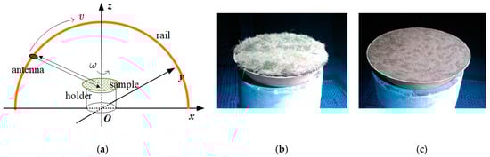
Figure 4.
(a) The schematic diagram of measurement set-up; (b) the grass sample; (c) the concrete sample.
The diagram in Figure 5 explains the measured data processing procedures, mainly involving background cancellation, transformation between near and far-field, as well as calibration. In detail, a standard metal ball with known RCS value has been used as the calibration body in the external calibration experiment at first. Considering the experiment space, the samples are measured at near field. The dotted-line box indicates the echoes received by antenna. Through background cancellation, the echo power is improved by a space filter, and converted to far-field with the support of antenna pattern and position compensation data. The measured sample RCSs are gathered in different azimuth angles and normalized by employing the calibration factor of the standard body. Hence normalized RCSs are obtained by averaging these data in different measuring conditions, which is equal to the backscatter coefficients in numeral.
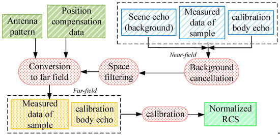
Figure 5.
The flow diagram of measured data processing procedures.
3.2. Space-time Coupled Clutter
With the SAR travelling at speed, the Doppler ranges from to with the relative motions between scene and radar, where ( represents the wave length). In another word, the frequency band of ground clutter spreads to wide [46,48]. It is reflected by the ground clutter distributing across the space-time domain, which is known as space-time coupling. Referring to Section 2.1, we deduce the space frequency and Doppler of ground clutter in rectangular coordinates as
where is the Pulse Repetition Interval (PRI) and denotes the element spacing in ULA.
Drawing on the traditional STAPs, is employed to describe the linearity between and given as when [49] (pp. 17–19). In case of N elements and K pulses in a Coherent Process Interval (CPI), ground clutter in each cell is
satisfies where is introduced to account the clutter intensity. Obviously, is almost decided by in the cell at . Hence the steering vectors are expressed as
Referring to Section 2.2, we define the clutter in each cell as
which could also be expressed in the form of a Kronecker product:
In practical operation, the clutter covariance matrix could be estimated by
to approach where
We notice that the estimation decouples from the IID training samples. In other words, it focuses on modelling the clutter with the aid of topography knowledge of runways to obtain reliable , which offers an unprecedented idea as the preliminary of STAP.
4. Clutter-Analysis-Based STAP
Clutter is required to be suppressed in the space-time domain by effective filtering. Traditional STAPs perform well under homogeneous clutter background by estimating clutter covariance from real echo directly. Notice that clutter echo from some range gates, which contains only one isotropic scattering surface (as Figure 2 depicts), is considered homogeneous, thus enough IID training samples could be gathered. Scattering cell division is not required considering the increasing computation. As for those range gates involving both lawn and concrete runways, we utilize the presented STAP to achieve exact for effective filter weight solution, considering the limited performance of some previous methods. Two approaches could be selected according to practical clutter cases, combining the characteristics and advantages of them.
According to all discussion above, the flow chart shows the processing steps involving the proposed STAP as well as traditional method for FOD detection:
See Figure 6, the clutter properties (homogeneous or not) could be known according to the corresponding range gates. To the homogeneous clutter echo, generated by lawn surface only, we employ traditional STAPs to estimate clutter covariance matrix from real IID samples directly (indicated by the green blocks in the flow diagram). Aided by the scene knowledge and a parameter-modified scattering model, we utilize the clutter-estimation-based STAP for effective suppression to the non-homogeneous clutter at those range gates involving runways and lawns, through scene-knowledge-aided division of scattering cells in xOy coordinates, transformation to polar coordinates (illustrated by pink), back-scattering coefficient acquirement based on the known grazing angles, and clutter echo deduction with the antenna pattern G, and estimation, as depicted by the blue blocks. Note that the dotted arrow in the figure implies the proposed STAP is real-clutter-decoupling.
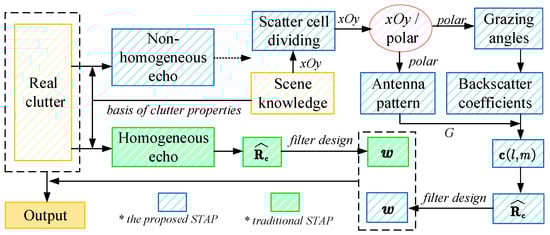
Figure 6.
The flow diagram of traditional and proposed Space-time Adaptive Processing (STAPs) application.
Before solving the filter weight, the space-time coupled echoes of FOD items are first deduced. For general analysis, we consider all possible targets as one or more scattering points. Taking a point target moving at in radial direction in the cell at as the example, the space frequency and Doppler are written as
and in space and time domains are expressed as [49]
Thus, the target echo is as the following equation shows [49]
in the condition that the scattering intensity and the amplitude satisfies . The optimal weight vector obeying Linearly Constrained Minimum Variance (LCMV) is:
which is known as the Wiener solution where = [50]. is preferable than in practice to avoid signal cancellation [49] (pp. 22,23). Thus, the target Doppler and azimuth are both acquired according to .
5. Experiments and Discussion
To evaluate the models, deductions, and conclusions above, experiments are presented according to the data setting in Section 5.1. The simulation results of the scattering cell division, the fitting results of Kulemin model, the MV spectrum of clutter, as well as the LCMV space-time filter are discussed in Section 5.2.
5.1. Dataset
As is presented in Figure 4, the grass and concrete samples are produced and measured on a rotating holder under the conditions illustrated in Table 2. Dataset 1 is the result of the grass sample and Dataset 2 is that of the concrete sample when the polarization is VV. The test data are displayed in Figure 7, when the grazing angle are controlled as 5, 10, and 15 degrees. Note that Figure 7a only shows a part of the data under −30 to 30 degrees.
Table 2.
The condition setting of backscatter coefficient measurement.
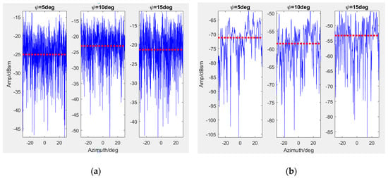
Figure 7.
Measured data and the statistical average values about the backscattering coefficients from Science and Technology on Electromagnetic Scattering Laboratory (a) Dataset 1 (b) Dataset 2 ().
The blue lines represent the data amplitude while the red dotted lines denote the average values of different azimuth cases at certain frequencies. Hence the data would be employed to modify Kulemin models by LS fitting. Referring to Section 3.1, the modified models at 10 GHz are firstly calculated and expressed as the implements to analyze scattering properties in low grazing angles.
5.2. Simulations and Discussion
Table 3 provides the simulation setting:
Table 3.
Parameter setting of simulations.
LS fitting results based on Dataset 1 and 2 are given in Figure 8a compared with the Kulemin models. They are considered reliable for the similar trends with the classical models. The coefficients of concrete are at least 36 dB less than those of the grass surface when the grazing angle is very small (≤10 degrees). Note that also plays as the foundation of , and , therefore we calculate of every cell covered by the SAR in Figure 8b to acquire the corresponding when . In this case, the grazing angles of cells increase from −0.2006 to 0.2006 and the scattering properties are displayed in Figure 9.
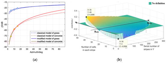
Figure 8.
(a) Comparison between traditional Kulemin model and the data fitting results; (b) of each cell ranges from −0.2006 to 0.2006, which constrains , and .
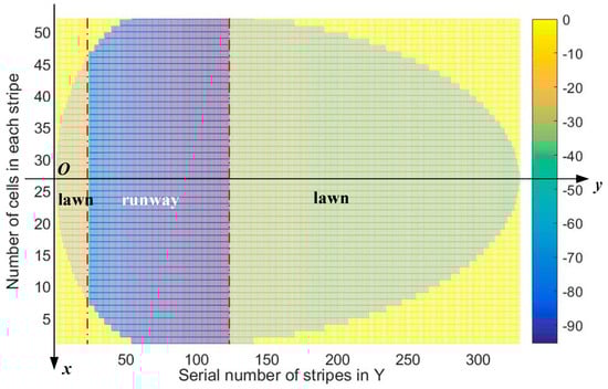
Figure 9.
Scattering properties within the radar coverage, on basis of the parameter-modified models in Figure 8a when the cell size is 0.5 m × 0.5 m.
With the side-looking SAR travelling, clutter Doppler is greatly expanded. FOD detection will be challenged because the target is severely fuzzed in the Doppler domain. As the basis of clutter suppression, the MV spectrum is ideal in evaluating the clutter visually and qualitatively. According to Section 3.2, we investigate the MV spectrum of clutter and noise on the space-time plane in Figure 10a–c when the noise power is −60 dBm, −80 dBm and −90 dBm. The ridge-shaped field reflects only when , known as the main clutter field, indicates where the clutter power mainly focuses. Red lines in Figure 10d–f provide the corresponding clutter suppression when utilizing a LCMV space-time filter.
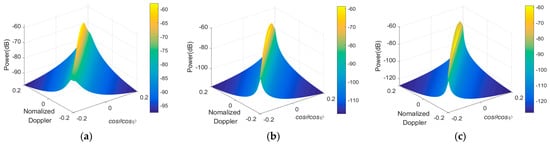
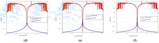
Figure 10.
The minimum variance (MV) power spectrum of clutter and noise shows space-time coupling indicated briefly by the ridge-shaped field when the noise power is (a) −60 dBm; (b) −80 dBm; (c) −90 dBm; the optimal response obeying linearly constrained minimum variance (LCMV) when the noise power is (d) −60 dBm; (e) −80 dBm; and (f) −90 dBm.
Obviously, the space-time coupled clutter is significantly suppressed to nearly −70 dB, −110 dB, and −120 dB, which is ideal referring to the corresponding red lines, which illustrate the power at clutter ridges achieving about 40 dB, 60 dB, and 70 dB higher than that on the other field of space-time plane. Taking a LCMV filter as the example, it works well for the following reasons: the power of the desired signal can be kept and the variance of the filter output is minimized as well. In fact, some filters obeying the other criteria (e.g., MSNR, MMSE) could also reach similar performances.
Aiming at qualitative analysis, we consider the six objects at 25th 0.5 × 0.5 m cell in 97th stripe (). Furthermore, we define the normalized Doppler as . Simulation results in azimuth and Doppler are respectively given in Figure 11.
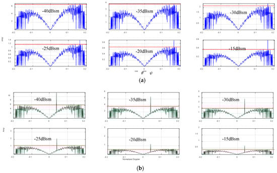
Figure 11.
Six object detections by LCMV filtering in (a) azimuth; (b) doppler under −60dBm noise environment.
Disturbed by −60 dBm noise, the simulations in Figure 11a demonstrate that false alarms are produced and the interference effective azimuth indication occurs when a target RCS is smaller than −30 dBsm. Meanwhile, we have also noticed that false alarms, generated by non-homogeneous scattering within radar coverage, exist all over the space-time plane especially in the azimuth domain. But the space-time filtering works well to all six targets in Doppler very clearly. Theoretically, motive objects are distinguished from the scattering cells in Doppler, which benefit the SAR system. In practical operation, a lower false alarm rate could be obtained by setting a threshold decision coefficient according to the characteristics and the distribution of clutter, which will be validated in future work.
In order to illustrate that the proposed method performs better than state-of-the-arts, samples from different range gates are utilized for filtering in the space-time domain. The number of range gates are expressed as where denotes rounding-up. Thus, there are 439 range gates covered by the SAR according to the parameter setting in Table 3. Figure 12 illustrated the MV spectrum brought by the error of clutter covariance matrix estimation, employing insufficient IID echo from some range gates. As a result, traditional estimation in Figure 13 cannot provide satisfactory clutter suppression when compared with the presented STAP. Obviously, estimation errors directly lead to unnecessary suppression on the space-time plane rather than the main clutter field, which always manifests as decreased SCNR of the filter output.
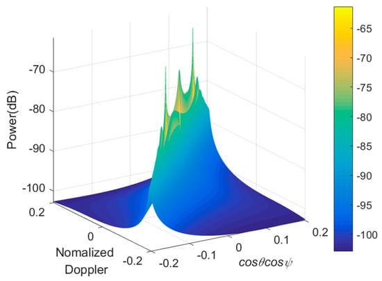
Figure 12.
MV spectrum of clutter estimated by samples of 20th to 50th range gates, where refers to both runway and lawn surface.
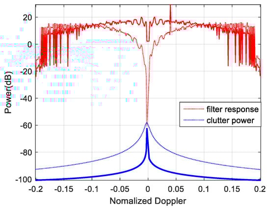
Figure 13.
Comparison between the proposed method and traditional processing aiming at a −20 dBsm object, where the solid lines indicate poor clutter suppression under −60 dBm noise.
6. Conclusions
STAP methods for moving FOD detection deserves more attention for many compelling advantages such as lower cost, more flexibility and higher resolution. However, the performance of the conventional statistical STAP meets great degradation under nonhomogeneous samples or environment. This paper proposed a clutter-analysis-based Space-time Adaptive Processing (STAP) method in order to obtain effective clutter suppression and moving FOD indication, under inhomogeneous clutter background. We first divided the radar coverage into equal scattering cells in the rectangular coordinates system rather than the polar ones. We then measured normalized RCSs within the X-band and employed the acquired results to modify the parameters of traditional models. Finally, we described the clutter expressions as responses of the scattering cells in the space and time domain to obtain the theoretical clutter covariance. Experimental results at 10 GHz indicated that FODs with a reflection higher than −30 dBsm could be effectively detected by a LCMV filter in azimuth when the noise was −60 dBm. It was also validated to indicate a −40 dBsm target in Doppler. The approach could obtain effective clutter suppression 60 dB deeper than the training-sample-coupled STAP under the same conditions.
Nevertheless, key problems confronted in real-world applications are presented for this STAP technique, which include false alarm effect, influence of spatial errors, and huge computational cost with exact cell division. Moreover, we also plan to investigate its performance under non-ideal conditions such as the presence of SAR yaw, steering vector mismatch, and complex terrains. Therefore, it is of great value to develop robust algorithms. We also realize that thinner item detection disturbed by strong interferences is the most difficult task in meeting practical demands. Future work will include testing on an airport runway to measure practicability and accuracy.
Author Contributions
Conceptualization, X.Y., X.Z. and W.J.; Funding acquisition, K.H.; Investigation, X.Y. and K.H.; Methodology, X.Y.; Resources, K.H. and W.J.; Measurements, Y.C.; Supervision, K.H., X.Z. and W.J.; Writing—original draft, X.Y.; Writing—review & editing, X.Y.
Funding
National Science Foundation of China (No. 61501481).
Acknowledgments
This work is funded by National Science Foundation of China under contract of No. 61501481.
Conflicts of Interest
The authors declare no conflict of interest.
Appendix A
In detail, we rewrite Equation (5) at first:
If measurements are taken, Equation (A1) can be expressed in the vector form as
where is collected in case of . Notice that is constant thus . Two functions are introduced as following:
then calculate the inner products among these two items and and put them into Equation (8):
We express Equation (A4) in form of matrix as
Hence both and can be solved based on Equation (A5)
then we could acquire backscattering coefficients in low grazing angles according to the modified model .
References
- CAAC. Manual on Preventing Foreign Object Debris (FOD); National Civil Aviation Administration of China: Beijing, China, 2009; pp. 1–2.
- Zhou, Y.; Xiong, J. Study on typical case analysis and preventive measures of runway invasion during take-off stage. J. Civ. Aviat. Flight Univ. Chin. 2010, 21, 32–35. [Google Scholar] [CrossRef]
- Patterson, J., Jr. Foreign Object Debris (FOD) Detection Research. Int. Airpt. Rev. 2008, 12, 22–27. [Google Scholar]
- iFerret on Scratch. Available online: https://www.sourcesecurity.com/news/stratech-iferret-assess-ground-surveillance-systems-co-7811-ga.19664.html/ (accessed on 24 January 2019).
- Tarsier®: Automatic Runway FOD Detection System. Available online: https://www.tarsierfod.com/ (accessed on 19 December 2018).
- FOD Finder™. Available online: https://www.xsightsys.com/index.php/fodetect/ (accessed on 4 January 2016).
- What Is FODetect? Available online: http://www.xsightsys.com/fodetect.html (accessed on 24 January 2018).
- CCTV Introduces the Foreign Object Debris System of Airport Runway in the Second Airport of Civil Aviation. Available online: http://news.carnoc.com/list/403/403257.html (accessed on 16 May 2017).
- Zeitler, A.; Lanteri, J.; Pichot, C. Folded reflect arrays with shaped beam pattern for foreign object debris detection on runways. IEEE Trans. Antennas Propag. 2010, 58, 3065–3068. [Google Scholar] [CrossRef]
- He, Y. Millimeter-Wave Radar FOD Detection Technology. Master’s Thesis, Beijing Jiaotong University, Beijing, China, 2014. [Google Scholar]
- Kang, Z.; Long, T. A New SAR Imaging Scheme in Foreign Object Debris Detection. In Proceedings of the International Congress on Image and Signal Processing, Chongqing, China, 16–18 October 2012; pp. 952–956. [Google Scholar] [CrossRef]
- Fan, M. Research on Foreign Object Debris Detection. Master’s Thesis, Beijing Jiaotong University, Beijing, China, June 2011. [Google Scholar]
- Mollo, G.; Napoli, R.D.; Naviglio, G. Multifrequency Experimental Analysis (10 to 77 GHz) on the Asphalt Reflectivity and RCS of FOD Targets. IEEE Geosci. Remote Sens. Lett. 2017, 14, 1441–1443. [Google Scholar] [CrossRef]
- Mazouni, K.; Zeitler, A.; Lanteri, J. 76.5 GHz millimeter-wave radar for foreign objects debris detection on airport runways. In Proceedings of the 8th European Radar Conference, Manchester, UK, 12–14 October 2011; pp. 317–326. [Google Scholar] [CrossRef]
- Mazouni, K.; Pichot, C.; Lantéri, J. 77 GHz offset reflectarray for FOD detection on airport runways. Int. J. Microw. Wirel. Technol. 2012, 4, 37–43. [Google Scholar] [CrossRef]
- Feil, P.; Menzel, W.; Nguyen, T.P. Foreign objects debris detection (FOD) on airport runways using a broadband 78 GHz sensor. In Proceedings of the European Radar Conference, Amsterdam, The Netherlands, 30–31 October 2008; pp. 451–454. [Google Scholar] [CrossRef]
- Futatsumori, S.; Morioka, K.; Kohmura, A. Design and Field Feasibility Evaluation of Distributed-Type 96 GHz FMCW Millimeter-Wave Radar Based on Radio-Over-Fiber and Optical Frequency Multiplier. J. Lightwave Technol. 2016, 34, 4835–4843. [Google Scholar] [CrossRef]
- Nsengiyumva, F.; Pichot, C.; Aliferis, I. Detection of debris (FOD) on runways in W-band: Relevance and validity domain of two-dimensional approaches. In Proceedings of the IEEE International Conference on Electromagnetics in Advanced Applications, Turin, Italy, 7–11 September 2015; pp. 117–120. [Google Scholar] [CrossRef]
- Jin, E.; Yan, D.; Zhang, Z. FOD Detection on Airport Runway with Clutter Map CFAR Plane Technique. In Communications, Signal Processing, and Systems; Springer: Berlin, Germany, 2012; Volume 202, pp. 335–342. [Google Scholar] [CrossRef]
- Wu, J.; Wang, H.; Yu, X. CFAR Detection Method in Multi-target Environments for Foreign Object Debris Surveillance Radar. In The Proceedings of the Second International Conference on Communications, Signal Processing, and Systems; Springer International Publishing: Berlin, Germany, 2014; Volume 246, pp. 533–540. [Google Scholar] [CrossRef]
- He, Z.; Miao, C.; Zhao, Y. Millimeter Wave Radar for FOD Detection on Airport Runway Based on SAR Principle. J. Microwav. 2017, S1, 230–233. [Google Scholar]
- Cong, X.; Liu, J.; Long, K. Millimeter-wave spotlight circular synthetic aperture radar (scsar) imaging for Foreign Object Debris on airport runway. In Proceedings of the IEEE International Conference on Signal Processing, Hangzhou, China, 19–23 October 2014; pp. 1968–1972. [Google Scholar] [CrossRef]
- Ao, D.; Wang, X.; Wang, H. Modeling of Foreign Objects Debris Detection Radar on Airport Runway. In Proceedings of the 2012 International Conference on Information Technology and Software Engineering; Springer: Berlin, Germany, 2013; pp. 115–123. [Google Scholar] [CrossRef]
- Kohmura, A.; Futatsumori, S.; Yonemoto, N.; Okada, K. Optical fiber connected millimeter-wave radar for FOD detection on runway. In Proceedings of the European Radar Conference, Nuremberg, Germany, 9–11 October 2013; pp. 41–44, ISBN 978-2-87487-033-0. [Google Scholar]
- Blacknell, D. Target detection in correlated SAR clutter. IEEE Proc. Radar Sonar Navig. 2002, 147, 9–16. [Google Scholar] [CrossRef]
- Soumekh, M.; Himed, B. SAR-MTI processing of multi-channel airborne radar measurement (MCARM) data. In Proceedings of the 2002 IEEE Radar Conference, Long Beach, CA, USA, 25 April 2002; pp. 24–28. [Google Scholar] [CrossRef]
- Sarkar, T.K.; Wang, H.; Park, S. A deterministic least-squares approach to space-time adaptive processing (STAP). IEEE Trans. Antennas Propag. 2001, 49, 91–103. [Google Scholar] [CrossRef]
- Reed, I.S.; Mallett, J.D.; Brennan, L.E. Rapid Convergence Rate in Adaptive Arrays. IEEE Trans. Aerosp. Electron. Syst. 1974, 10, 853–863. [Google Scholar] [CrossRef]
- Gerlach, K.; Blunt, S.D.; Picciolo, M.L. Robust adaptive matched filtering using the FRACTA algorithm. IEEE Trans. Aerosp. Electron. Syst. 2004, 40, 929–945. [Google Scholar] [CrossRef]
- Huang, L.; Thompson, E.A.; Schmithorst, V.; Holland, S.K.; Talavage, T.M. Partially Adaptive STAP Algorithm Approaches to Functional MRI. IEEE Trans. Biomed. Eng. 2009, 56, 518–521. [Google Scholar] [CrossRef]
- Ginolhac, G.; Forster, P.; Pascal, F.; Ovarlez, J.P. Performance of Two Low-Rank STAP Filters in a Heterogeneous Noise. IEEE Trans. Signal Process. 2012, 61, 57–61. [Google Scholar] [CrossRef]
- Fa, R.; Lamare, R.C.D.; Wang, L. Reduced-Rank STAP Schemes for Airborne Radar Based on Switched Joint Interpolation, Decimation and Filtering Algorithm. IEEE Trans. Signal Process. 2010, 58, 4182–4194. [Google Scholar] [CrossRef]
- Yang, Z.; Li, X.; Wang, H.; Fa, R. Knowledge-aided STAP with sparse-recovery by exploiting spatio-temporal sparsity. IET Signal Process. 2016, 10, 150–161. [Google Scholar] [CrossRef]
- Yang, K.; Bar-Shalom, Y.; Willett, P. Sparsity-Based STAP Using Alternating Direction Method with Gain/Phase Errors. IEEE Trans. Aerosp. Electron. Syst. 2017, 99. [Google Scholar] [CrossRef]
- Riedl, M.; Potter, L.C. Knowledge-Aided Bayesian Space-Time Adaptive Processing. IEEE Trans. Aerosp. Electron. Syst. 2018, 54, 1850–1861. [Google Scholar] [CrossRef]
- Wang, P.; Li, H.; Himed, B. A Bayesian Parametric Test for Multichannel Adaptive Signal Detection in Nonhomogeneous Environments. IEEE Signal Process. Lett. 2010, 17, 351–354. [Google Scholar] [CrossRef]
- Wen, C.; Peng, J.; Zhou, Y.; Wu, J. Enhanced Three-Dimensional Joint Domain Localized STAP for Airborne FDA-MIMO Radar under Dense False-Target Jamming Scenario. IEEE Sens. J. 2018, 18, 4154–4166. [Google Scholar] [CrossRef]
- Zhang, S.; He, Z.; Jun, L.; Wang, Y. A Robust Colored-loading Factor Optimization Approach for KA-STAP. J. Electron. Inf. Technol. 2016, 38, 1942–1949. [Google Scholar] [CrossRef]
- Wu, Y.; Wang, T.; Wu, J.; Duan, J. Robust training samples selection algorithm based on spectral similarity for space–time adaptive processing in heterogeneous interference environments. IET Radar Sonar Navig. 2015, 9, 778–782. [Google Scholar] [CrossRef]
- Han, S.; Fan, C.; Huang, X. A novel training sample selection method for STAP based on clutter sparse recovery. In Proceedings of the IEEE Progress in Electromagnetic Research Symposium, 2016 Congress on Image and Signal Processing, Shanghai, China, 8–11 August 2016. [Google Scholar] [CrossRef]
- Wu, J.; Wang, X.; Wang, H. Radar echo modeling of Foreign Objects Debris detection on airport runways. J. Terahertz Sci. Electron. Inf. Technol. 2013, 11, 917–921. [Google Scholar] [CrossRef]
- Mehdi, G.; Miao, J. Millimetre Wave FMCW Radar for Foreign Object Debris (FOD) Detection at Airport Runways. In Proceedings of the 9th International Conference, Applied Science & Technology, Islamabad, Pakistan, 9–12 January 2012; pp. 407–412. [Google Scholar] [CrossRef]
- Rao, N.; Chen, X.; Zhou, J. Research on Ground Modelling of Airborne Cognitive Radar Based on Digital Elevation Model Data. J. Univ. Electron. Sci. Technol. Chin. 2016, 45, 511–519. [Google Scholar] [CrossRef]
- Sun, G.; He, Z.; Tong, J.; Zhang, X. Knowledge-Aided Covariance Matrix Estimation via Kronecker Product Expansions for Airborne STAP. IEEE Geosci. Remote Sens. Lett. 2018, 15, 1–5. [Google Scholar] [CrossRef]
- AC 150/5220-24 Airport Foreign Object Debris Detection Equipment. Available online: https://www.faa.gov/regulations_policies/advisory_circulars/index.cfm/go/document.information/documentID/99719 (accessed on 30 September 2009).
- Brennan, L.E.; Malle, J.D.; Reed, L.S. Theory of Adaptive Radar. IEEE Trans. Aerosp. Electron. Syst. 1973, 9, 237–252. [Google Scholar] [CrossRef]
- Oh, Y.; Sarabandi, K.; Ulaby, F.T. An empirical model and an inversion technique for radar scattering from bare soil surfaces. IEEE Trans. Geosci. Remote Sens. 1992, 30, 370–381. [Google Scholar] [CrossRef]
- Klemm, R. Applications of Space-Time Adaptive Processing; IET Digital Library: London, UK, 2004; pp. 154–196. ISBN 9780852969243. [Google Scholar]
- Qin, L. Research on Robust Space-Time Adaptive Processing for Airborne Radar. Ph.D. Thesis, National University of Defence Technology, Changsha, China, June 2017. [Google Scholar]
- Zhang, X.; Li, Y.; Yang, X.; Long, T. Sub-Array Weighting UN-MUSIC: A Unified Framework and Optimal Weighting Strategy. IEEE Signal Process. Lett. 2014, 21, 871–874. [Google Scholar] [CrossRef]
© 2019 by the authors. Licensee MDPI, Basel, Switzerland. This article is an open access article distributed under the terms and conditions of the Creative Commons Attribution (CC BY) license (http://creativecommons.org/licenses/by/4.0/).