An Improved Normalized Mutual Information Variable Selection Algorithm for Neural Network-Based Soft Sensors


Abstract
1. Introduction
- (1)
- The proposed algorithm performs variable selection by combining the NMI and training accuracy of neural networks.
- (2)
- TS is used as an auxiliary optimization method, and it effectively prevents the proposed algorithm from falling into local optimums.
- (3)
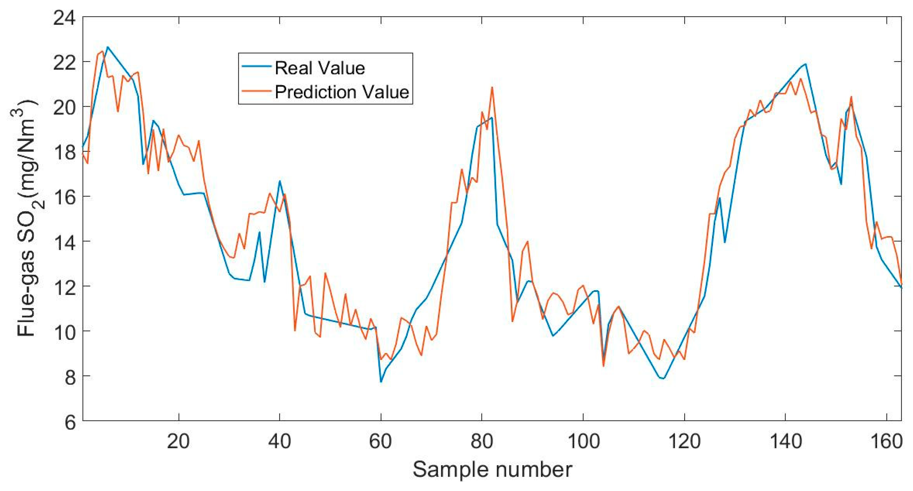
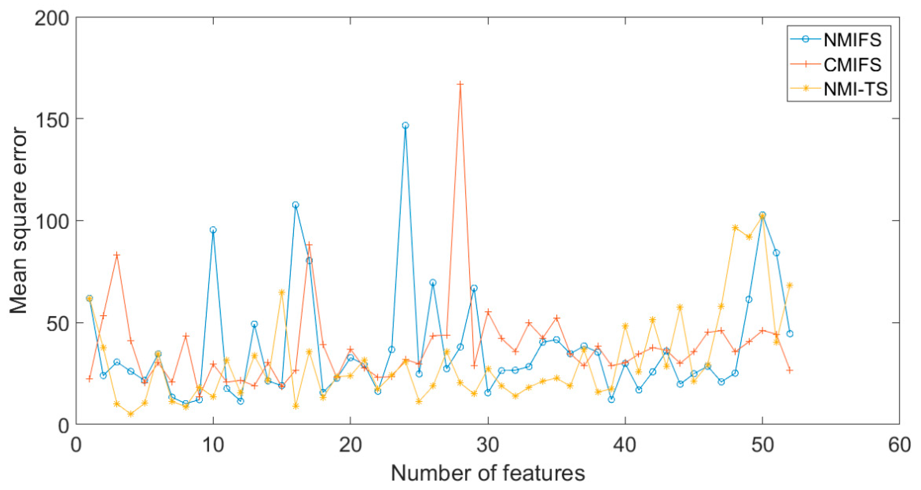
- The developed soft sensor is applied to predict the sulfur dioxide (SO2) emissions of flue gas in a practical power plant, and it has better performance than other algorithms.
2. Theoretical Overview
2.1. Input Variable Selection Techniques
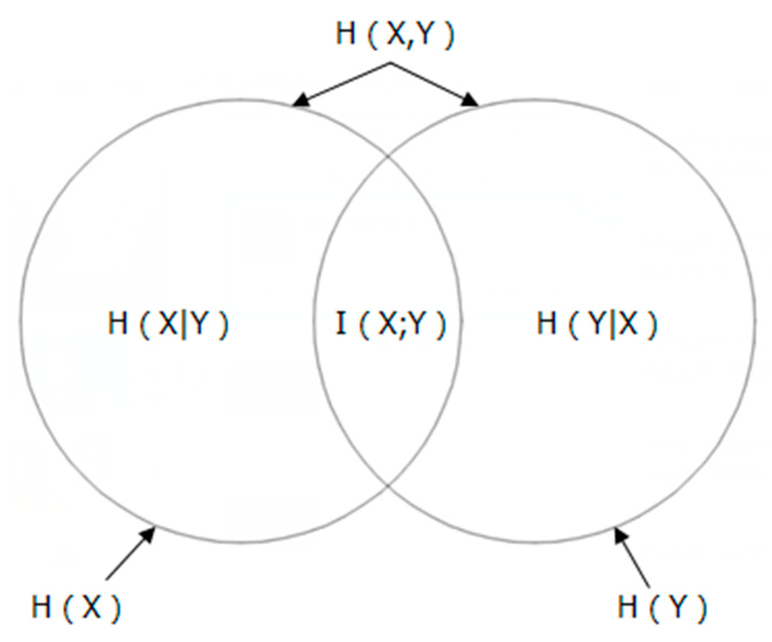
2.2. Mutual Information (MI)
- Symmetry: I(X;Y) = I (Y;X).The information extracted from Y about X is of the same amount as the information extracted from X about Y. The only difference between them is the angle of the observer.
- Positive: I(X;Y) ≥ 0. For all extracting information, the worst case scenario is that there is no information, that is I(X;Y) = 0
- Extremum: I(X;Y) ≤ H(X), I(Y;X) ≤ H(Y). The amount of information extracted from one event about another is at most equal to the entropy of the other event, and does not exceed the amount of information contained in this other event itself.
2.3. Tabu Search
- Step 1
- Generate an initial solution x ∈ X, set x* = x, T = ∅, define amnesty rule as A(x) = C(x*), iterations k = 0.
- Step 2
- k = k + 1, if k > MK (MK is the maximum number of iterations), Stop the search.
- Step 3
- C() max{C(x),}, if A(x) < C(), set x = , jump to Step 5.
- Step 4
- C() max{C(x),}, set x = .
- Step 5
- If C(x) < C(x*), set x = x*, C(x*) = C(x), A(x) = C(x*).
- Step 6
- Add x* to tabu list, release the solution that reaches the tabu length and return to Step 2
3. Design and Analysis of Algorithms
3.1. Proposed Methods for Feature Selection
- Step 1
- Evaluate I(Y; pj); for each variable in P, Select the variable corresponding to the biggest I(Y; pj) as the starting point.
- Step 2
- If or , Stop the search.
- Step 3
- The variables satisfying the tabu length were taken from S and added to P.
- Step 4
- Evaluate for each variable in P.
- Step 5
- Sort the variables in P by , select the first N variables and put them in neighborhood.
- Step 6
- Evaluate (fitness value) for each variable in the neighborhood.
- Step 7
- Select the variable corresponding to the smallest as the optimal solution of this iteration
- Step 8
- Put the other variables in S and return to Step 2.
| Algorithm 1: Pseudo-code of NMI-TS algorithm |
| Input: dataset {P, Y} Results: new dataset A after selection |
| While P ≠ ∅ or S ≠ ∅ release the solution that reaches the tabu length; j = 1; While j <= the length of P J = j + 1; end Sort the variables in P by Bj from largest to smallest and select the first N variables, put them in set M; N = 1; While n <= N Evaluate λn for nth variable in M; (by using Algorithm 2) n = n + 1; end Select the variable corresponding to the smallest λn and add it to A, Put the other variables in S; End |
3.2. Subroutine of Cross-Validation (CV)
| Algorithm 2: Subroutine of CV |
| Input: dataset {A, Y} Results: fitness value λn Divide{A,Y}into k disjoint sub-datasets{A1,Y1},{A2,Y2},{A3,Y3},……,{Ak,Yk}; For p = 1:k Set A as the input variable, Y as the output variable; Train a new ANN with dataset {A,Y}={A,Y}-{Ak,Yk}; Validate the dataset {Ak,Yk} on the new ANN and the MSE denoted as MSEp; End |
4. Numerical Examples
4.1. Experimental Setting
- (1)
- Model size (M.S): The number of input variables selected by the algorithm.
- (2)
- MSE: During the whole modeling process, part of the data is used for modeling, and the other part is used to verify the accuracy of the model. We recorded MSE between the predicted and desired output to evaluate the prediction accuracy of the model.
- (3)
- Coefficient of determination : the square of the sample correlation coefficients between the actual and predicted values.
- (4)
- Positive wrong selection (WS+): The ratio of unselected valid variables to all valid variables and the number of unselected valid variables.
- (5)
- Negative wrong selection (WS−):The ratio and number of irrelevant variables in the results.
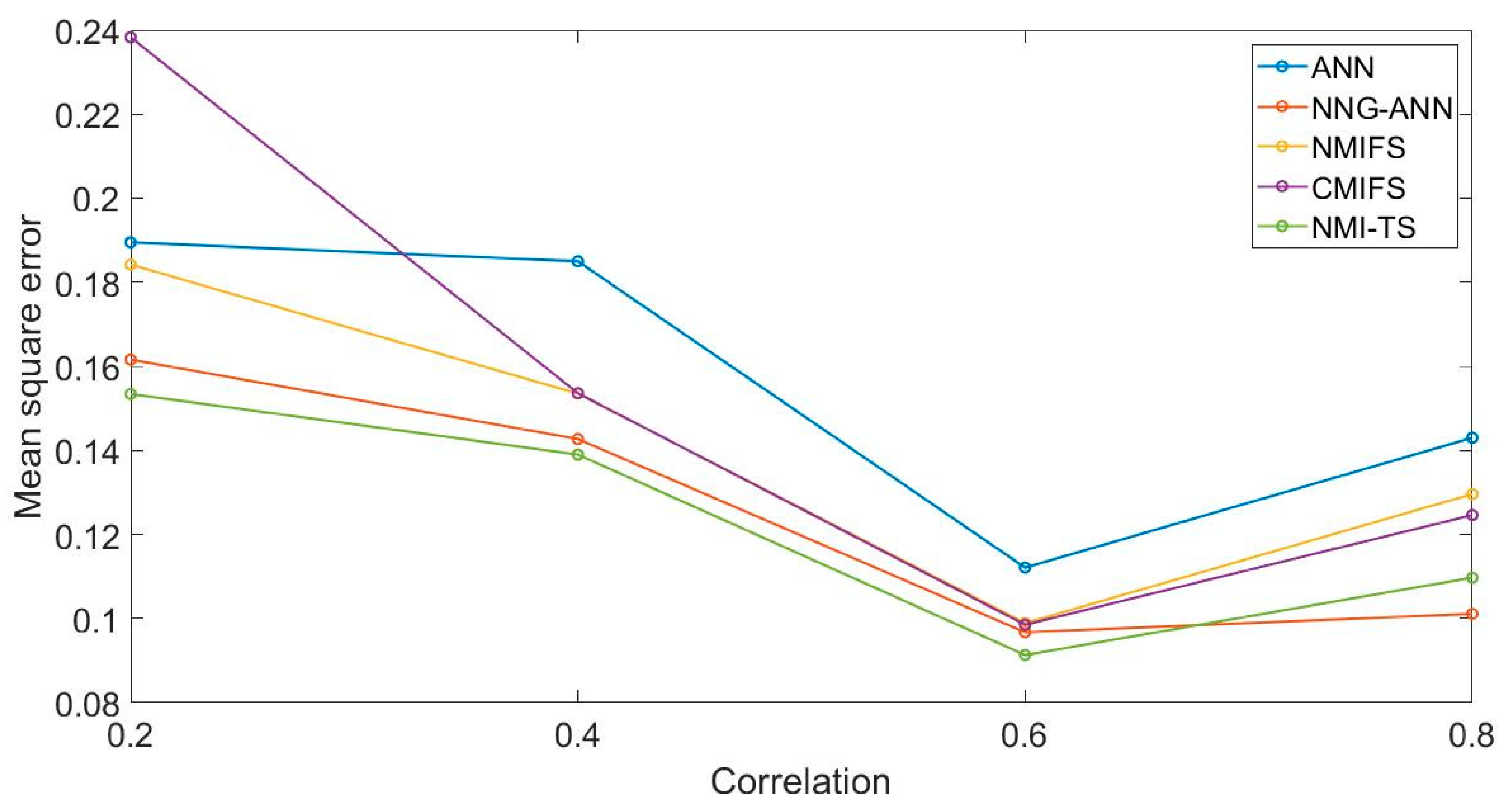
4.2. Case 1
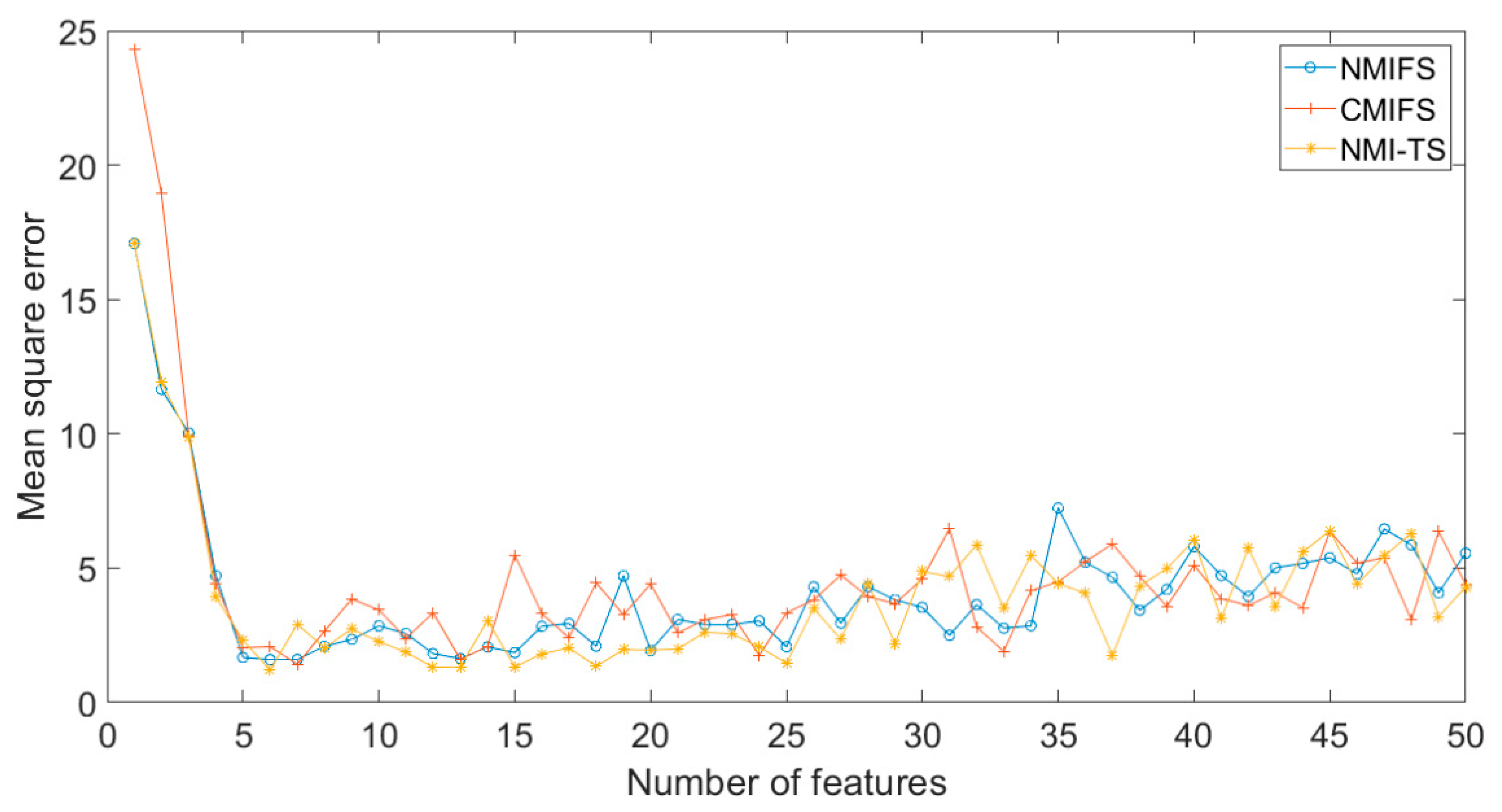
4.3. Case 2
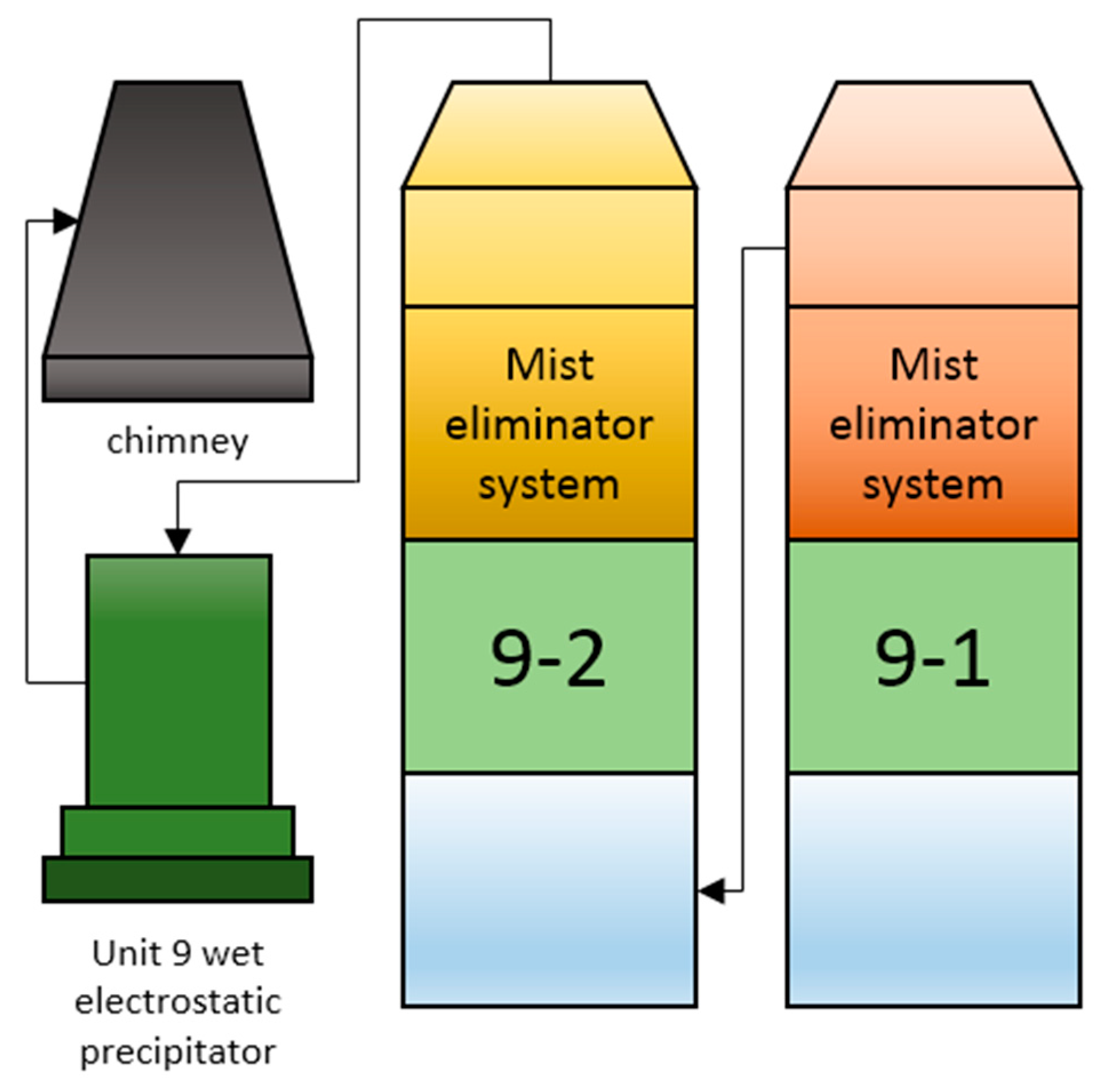
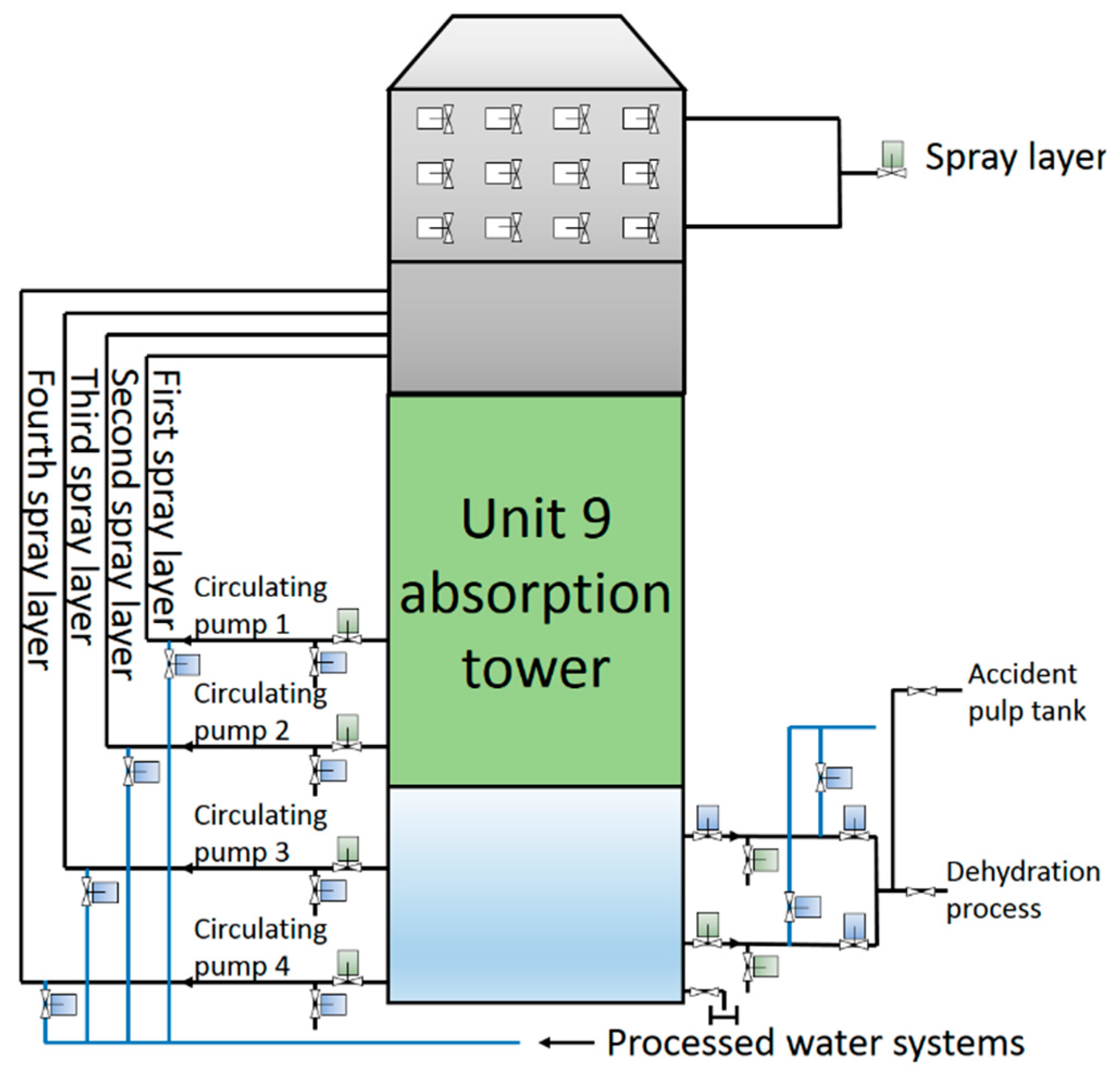
5. Application to Actual Desulfurization Process
5.1. Desulfurization Technology of the Power Plant
5.2. Expriment’s Design and Results
6. Conclusions
Author Contributions
Funding
Conflicts of Interest
Appendix A

| Number | Input Variable | Units |
|---|---|---|
| 1 | #9-1 Circulating SP current | A |
| 2 | #9-2 Circulating SP current | A |
| 3 | #9-3 Circulating SP current | A |
| 4 | #9-4 Circulating SP current | A |
| 5 | #9Cycle SP E B phase current | A |
| 6 | #9Cycle SP G B phase current | A |
| 7 | AT gypsum DP 2′s current | A |
| 8 | AT gypsum DP 1′s current | A |
| 9 | Gypsum slurry DP A’s current | A |
| 10 | Water ring vacuum pump’s current | A |
| 11 | #9AT’s inlet flue-gas temperature | K |
| 12 | #9AT’s outlet flue-gas temp.1 | K |
| 13 | #9AT’s outlet flue-gas temp. 2 | K |
| 14 | #9AT’s outlet flue-gas temp.3 | K |
| 15 | #9-2 AT outlet temperature 1 | K |
| 16 | #9-2 AT outlet temperature 2 | K |
| 17 | #9 AT’s gypsum slurry density | kg/m3 |
| 18 | Limestone slurry density | kg/m3 |
| 19 | #9 Furnace chimney inlet net flue-gas pressure | kPa |
| 20 | #9-2 AT outlet pressure | kPa |
| 21 | AT gypsum DP 1′s inlet pressure | kPa |
| 22 | AT gypsum DP 2′s inlet pressure | kPa |
| 23 | #9 Gypsum slurry cyclone’s inlet pressure | kPa |
| 24 | Gypsum SP to #9 AT tube’s pressure | kPa |
| 25 | Generator Power | kW |
| 26 | #9 Absorber liquid level’s value | m |
| 27 | #9-2 AT liquid level 1 | m |
| 28 | #9-2 AT liquid level 2 | m |
| 29 | #9-2 AT liquid level 3 | m |
| 30 | Gypsum slurry tank’s level | m |
| 31 | Belt dewatering machine A’s gypsum filter cake thickness | m |
| 32 | #9Furnace’s original flue-gas SO2 | mg/Nm3 |
| 33 | #9-1AT outlet’s flue-gas SO2 | mg/Nm3 |
| 34 | #9 Furnace original concentration of flue-gas and dust | mg/Nm3 |
| 35 | #9 Furnace original flue-gas NOx | mg/Nm3 |
| 36 | #9 Furnace original flue-gas O2 | mg/Nm3 |
| 37 | #9-1 AT outlet flue-gas O2 | mg/Nm3 |
| 38 | Limestone slurry to #9 AT flow | Nm3/h |
| 39 | #9-2AT’s feed flow | Nm3/h |
| 40 | Total air volume | Nm3/h |
| 41 | Total coal | Nm3/h |
| 42 | #9Furnace’s chimney inlet net flue-gas flow | Nm3/h |
| 43 | #9 original smoke flow | Nm3/h |
| 44 | #9 AT gypsum’s slurry flow | Nm3/h |
| 45 | AT gypsum DP 1′s speed feedback | r/s |
| 46 | AT gypsum DP 2′s speed feedback | r/s |
| 47 | Gypsum SP A’s speed feedback | r/s |
| 48 | Vacuum belt dewatering machine’s speed feedback | r/s |
| 49 | #9 AT gypsum’s slurry pH value | |
| 50 | #9-2AT’s pH value 1 | |
| 51 | Unit 9 desulfurization efficiency | |
| 52 | Intermediate value of desulfurization efficiency of Unit 9 |
References
- Paulsson, D.; Gustavsson, R.; Mandenius, C.F. A soft sensor for bioprocess control based on sequential filtering of metabolic heat signals. Sensors 2014, 14, 17864–17882. [Google Scholar] [CrossRef] [PubMed]
- Chen, K.; Liang, Y.; Gao, Z.; Liu, Y. Just-in-time correntropy soft sensor with noisy data for industrial silicon content prediction. Sensors 2017, 17, 1830. [Google Scholar] [CrossRef] [PubMed]
- Kaneko, H.; Arakawa, M.; Funatsu, K. Development of a new soft sensor method using independent component analysis and partial least squares. Aiche J. 2010, 55, 87–98. [Google Scholar] [CrossRef]
- Ahmed, F.; Nazir, S.; Yeo, Y.K. A recursive PLS-based soft sensor for prediction of the melt index during grade change operations in HDPE plant. Korean J. Chem. Eng. 2009, 26, 14–20. [Google Scholar] [CrossRef]
- Wang, D.; Liu, J.; Srinivasan, R. Data-driven soft sensor approach for quality prediction in a refining process. IEEE Trans. Ind. Inform. 2010, 6, 11–17. [Google Scholar] [CrossRef]
- Xing, H.; Jun, J.; Kaixin, L.; Zengliang, G.; Yi, L. Soft sensing of silicon content via bagging local semi-supervised models. Sensors 2019, 19, 3814. [Google Scholar]
- Yuan, X.; Huang, B.; Wang, Y.; Yang, C.; Gui, W. Deep learning-based feature representation and its application for soft sensor modeling with variable-wise weighted SAE. IEEE Trans. Ind. Inform. 2018, 14, 3235–3243. [Google Scholar] [CrossRef]
- Mambou, S.; Krejcar, O.; Kuca, K.; Selamat, A. Novel cross-view human action model recognition based on the powerful view-invariant features technique. Future Internet 2018, 10, 89. [Google Scholar] [CrossRef]
- Mambou, S.; Krejcar, O.; Maresova, P.; Selamat, A.; Kuca, K. Novel hand gesture alert system. Appl. Sci. 2019, 9, 3419. [Google Scholar] [CrossRef]
- Feil, B.; Abonyi, J.; Pach, P.; Nemeth, S.; Arva, P.; Nemeth, M.; Nagy, G. Semi-mechanistic models for state-estimation–soft sensor for polymer melt index prediction. In Artificial Intelligence and Soft Computing; Springer: Berlin/Heidelberg, Germany, 2004; Volume 3070, pp. 1111–1117. [Google Scholar]
- Ko, Y.D.; Shang, H. A neural network-based soft sensor for particle size distribution using image analysis. Powder Technol. 2011, 212, 359–366. [Google Scholar] [CrossRef]
- Shakil, M.; Elshafei, M.; Habib, M.A.; Maleki, F.A. Soft sensor for NOx and O2 using dynamic neural networks. Comput. Electr. Eng. 2009, 35, 578–586. [Google Scholar] [CrossRef]
- Bo, C.M.; Li, J.; Sun, C.Y.; Wang, Y.R. The application of neural network soft sensor technology to an advanced control system of distillation operation. In Proceedings of the International Joint Conference on Neural Networks, Portland, OR, USA, 20–24 July 2003; pp. 1054–1058. [Google Scholar]
- Jiesheng, W.; Shuang, H.; Nana, S. Features extraction of flotation froth images and BP neural network soft-sensor model of concentrate grade optimized by shuffled cuckoo searching algorithm. Sci. World J. 2014, 2014, 17. [Google Scholar]
- Le, Y.; Zhiqiang, G. Big data quality prediction in the process industry: A distributed parallel modeling framework. J. Process. Control 2018, 68, 1–13. [Google Scholar]
- Xinyu, Z.; Zhiqiang, G. Local parameter optimization of LSSVM for industrial soft sensing with big data and cloud implementation. IEEE Trans. Ind. Inform. 2019, 1. [Google Scholar] [CrossRef]
- Greenland, S. Modeling and variable selection in epidemiologic analysis. Am. J. Public Health 1989, 79, 340–349. [Google Scholar] [CrossRef] [PubMed]
- Hui, Z.; Hastie, T. Addendum: Regularization and variable selection via the elastic net. J. R. Stat. Soc. 2005, 67, 768. [Google Scholar]
- Raftery, A.E.; Dean, N. Variable selection for model-based clustering. J. Am. Stat. Assoc. 2017, 101, 168–178. [Google Scholar] [CrossRef]
- Wang, J.L.; Zhang, J.; Wang, X.X. A data driven cycle time prediction with feature selection in a semiconductor wafer fabrication system. IEEE Trans. Semicond. Manuf. 2018, 31, 173–182. [Google Scholar] [CrossRef]
- Mcnitt-Gray, M.F.; Huang, H.K.; Sayre, J.W. Feature selection in the pattern classification problem of digital chest radiograph segmentation. IEEE Trans. Med. Imaging 1995, 14, 537. [Google Scholar] [CrossRef]
- Le, Y.; Zhiqiang, G. Variable selection for nonlinear soft sensor development with enhanced binary differential evolution algorithm. Control Eng. Pract. 2018, 72, 68–82. [Google Scholar]
- Zhiqiang, G.; Zhihuan, S. A comparative study of just-in-time-learning based methods for online soft sensor modeling. Chemom. Intell. Lab. Syst. 2010, 104, 306–317. [Google Scholar]
- Sun, K.; Liu, J.; Kang, J.L.; Jang, S.S.; Wong, S.H.; Chen, D.S. Development of a variable selection method for soft sensor using artificial neural network and nonnegative garrote. J. Process Control 2014, 24, 1068–1075. [Google Scholar] [CrossRef]
- Frénay, B.; Doquire, G.; Verleysen, M. Is mutual information adequate for feature selection in regression? Neural Netw. 2013, 48, 1–7. [Google Scholar] [CrossRef] [PubMed]
- Battiti, R. Using mutual information for selecting features in supervised neural net learning. IEEE Trans. Neural Netw. 1994, 5, 537–550. [Google Scholar] [CrossRef] [PubMed]
- Soofi, E.S.; Retzer, J.J. Information importance of explanatory variables. In IEE Conference in Honor of Arnold Zellner: Recent Developments in the Theory, Method and Application of Entropy Econometrics; IEE: Washington, DC, USA, 2003. [Google Scholar]
- Hanchuan, P.; Fuhui, L.; Chris, D. Feature selection based on mutual information: Criteria of max-dependency, max-relevance, and min-redundancy. IEEE Trans. Pattern Anal. Mach. Intell. 2005, 27, 1226–1238. [Google Scholar] [CrossRef] [PubMed]
- Estévez, P.A.; Michel, T.; Perez, C.A.; Zurada, J.M. Normalized mutual information feature selection. IEEE Trans. Neural Netw. 2009, 20, 189–201. [Google Scholar] [CrossRef] [PubMed]
- Bennasar, M.; Hicks, Y.; Setchi, R. Feature selection using joint mutual information maximisation. Expert Syst. Appl. 2015, 42, 8520–8532. [Google Scholar] [CrossRef]
- Novovicová, J.; Somol, P.; Haindl, M.; Pudil, P. Conditional mutual information based feature selection for classification task. In Iberoamerican Congress on Pattern Recognition; Springer: Berlin/Heidelberg, Germany, 2007; Volume 4756, pp. 417–426. [Google Scholar]
- Zhang, H.; Sun, G. Feature selection using tabu search method. Pattern Recognit. 2002, 35, 701–711. [Google Scholar] [CrossRef]
- Pachecoaab, J. A variable selection method based on tabu search for logistic regression models. Eur. J. Oper. Res. 2009, 199, 506–511. [Google Scholar] [CrossRef]
- Osman, I.H. Metastrategy simulated annealing and tabu search algorithms for the vehicle routing problem. Ann. Oper. Res. 1993, 41, 421–451. [Google Scholar] [CrossRef]
- Lin, W.M.; Cheng, F.S.; Tsay, M.T. An improved tabu search for economic dispatch with multiple minima. IEEE Power Eng. Rev. 2007, 22, 70. [Google Scholar] [CrossRef]
- Enrique, R.; Josep María, S. Performing feature selection with multilayer perceptrons. IEEE Trans. Neural Netw. 2008, 19, 431–441. [Google Scholar]
- Peterson, L.E. K-nearest neighbor. Scholarpedia 2009, 4, 1883. [Google Scholar] [CrossRef]
- Kraskov, A.; Stögbauer, H.; Grassberger, P. Estimating mutual information. Phys. Rev. E Stat. Nonlinear Soft Matter Phys. 2004, 69, 066138. [Google Scholar] [CrossRef] [PubMed]
- Fukunaga, K. Introduction to Statistical Pattern Recognition; Elsevier: Amsterdam, The Netherlands, 2013. [Google Scholar]
- Khaksar, W.; Hong, T.S.; Khaksar, M.; Motlagh, O. A fuzzy-tabu real time controller for sampling-based motion planning in unknown environment. Appl. Intell. 2014, 41, 870–886. [Google Scholar] [CrossRef]
- Hongxing, W.; Wang, B.; Wang, Y.; Shao, Z.; Chan, K.C.C. Staying-alive path planning with energy optimization for mobile robots. Expert Syst. Appl. 2012, 39, 3559–3571. [Google Scholar]
- Faris, H.; Aljarah, I.; Mirjalili, S. Improved monarch butterfly optimization for unconstrained global search and neural network training. Appl. Intell. 2017, 48, 445–464. [Google Scholar] [CrossRef]
- Pan, C.C.; Bai, J.; Yang, G.K.; Wong, S.H.; Jang, S.S. An inferential modeling method using enumerative PLS based nonnegative garrote regression. J. Process Control 2012, 22, 1637–1646. [Google Scholar] [CrossRef]
- Friedman, J.H. Multivariate adaptive regression splines. Ann. Stat. 1991, 19, 1–67. [Google Scholar] [CrossRef]


| M.S | MSE | WS+ | WS− | ||
|---|---|---|---|---|---|
| ANN | 20 | 0.1895 | 0.8747 | N/A | N/A |
| NNG-ANN | 13 | 0.1616 | 0.8960 | 10.0%/1 | 30.7%/4 |
| NMIFS | 16 | 0.1842 | 0.8781 | 10.0%/1 | 43.7%/7 |
| CMIFS | 17 | 0.1617 | 0.8941 | 0 | 41.2%/7 |
| NMI-TS | 11 | 0.1534 | 0.9003 | 0 | 9.1%/1 |
| M.S | MSE | WS+ | WS- | ||
|---|---|---|---|---|---|
| ANN | 50 | 3.8992 | 0.9216 | N/A | N/A |
| NNG-ANN | 20 | 2.0691 | 0.9598 | 20.0%/1 | 80.0%/16 |
| NMIFS | 6 | 1.5943 | 0.9687 | 100.0%/5 | 100.0%/5 |
| CMIFS | 7 | 1.4257 | 0.9723 | 60.0%/3 | 71.4%/5 |
| NMI-TS | 6 | 1.2076 | 0.9764 | 20.0%/1 | 33.3%/2 |
| M.S | MSE | ||
|---|---|---|---|
| ANN | 52 | 23.4420 | 0.5124 |
| NNG-ANN | 10 | 8.8661 | 0.8243 |
| NMIFS | 8 | 10.2379 | 0.7710 |
| CMIFS | 9 | 13.6934 | 0.7225 |
| NMI-TS | 4 | 5.1309 | 0.8272 |
| Number | Input Variable | Units |
|---|---|---|
| 3 | #9-3 Circulating SP current | A |
| 33 | #9-1AT outlet’s flue gas SO2 | mg/Nm3 |
| 38 | Limestone slurry to #9 AT flow | Nm3/h |
| 50 | #9-2AT’s pH value 1 |
© 2019 by the authors. Licensee MDPI, Basel, Switzerland. This article is an open access article distributed under the terms and conditions of the Creative Commons Attribution (CC BY) license (http://creativecommons.org/licenses/by/4.0/).
Share and Cite
Sun, K.; Tian, P.; Qi, H.; Ma, F.; Yang, G. An Improved Normalized Mutual Information Variable Selection Algorithm for Neural Network-Based Soft Sensors. Sensors 2019, 19, 5368. https://doi.org/10.3390/s19245368
Sun K, Tian P, Qi H, Ma F, Yang G. An Improved Normalized Mutual Information Variable Selection Algorithm for Neural Network-Based Soft Sensors. Sensors. 2019; 19(24):5368. https://doi.org/10.3390/s19245368
Chicago/Turabian StyleSun, Kai, Pengxin Tian, Huanning Qi, Fengying Ma, and Genke Yang. 2019. "An Improved Normalized Mutual Information Variable Selection Algorithm for Neural Network-Based Soft Sensors" Sensors 19, no. 24: 5368. https://doi.org/10.3390/s19245368
APA StyleSun, K., Tian, P., Qi, H., Ma, F., & Yang, G. (2019). An Improved Normalized Mutual Information Variable Selection Algorithm for Neural Network-Based Soft Sensors. Sensors, 19(24), 5368. https://doi.org/10.3390/s19245368