Face Detection Ensemble with Methods Using Depth Information to Filter False Positives


Abstract
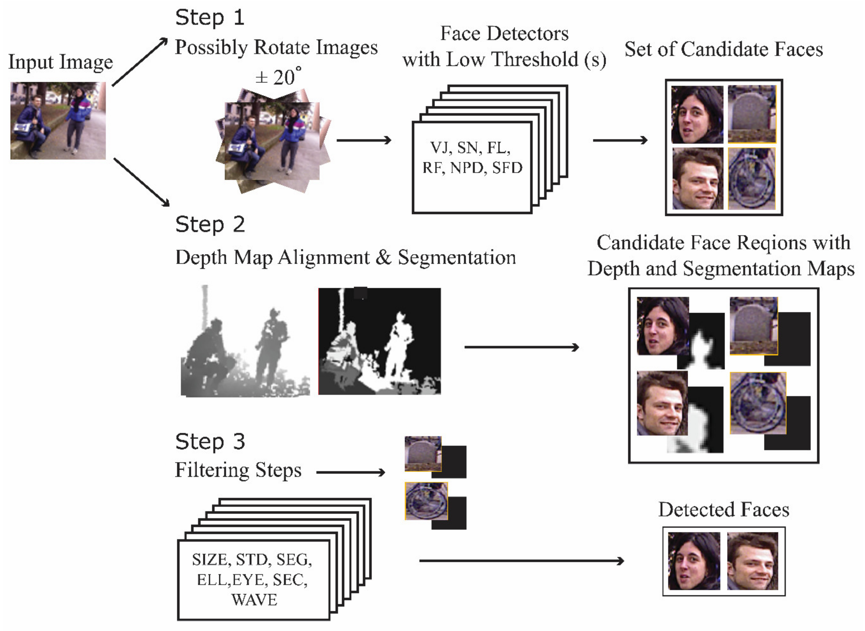
:1. Introduction
2. Materials and Methods
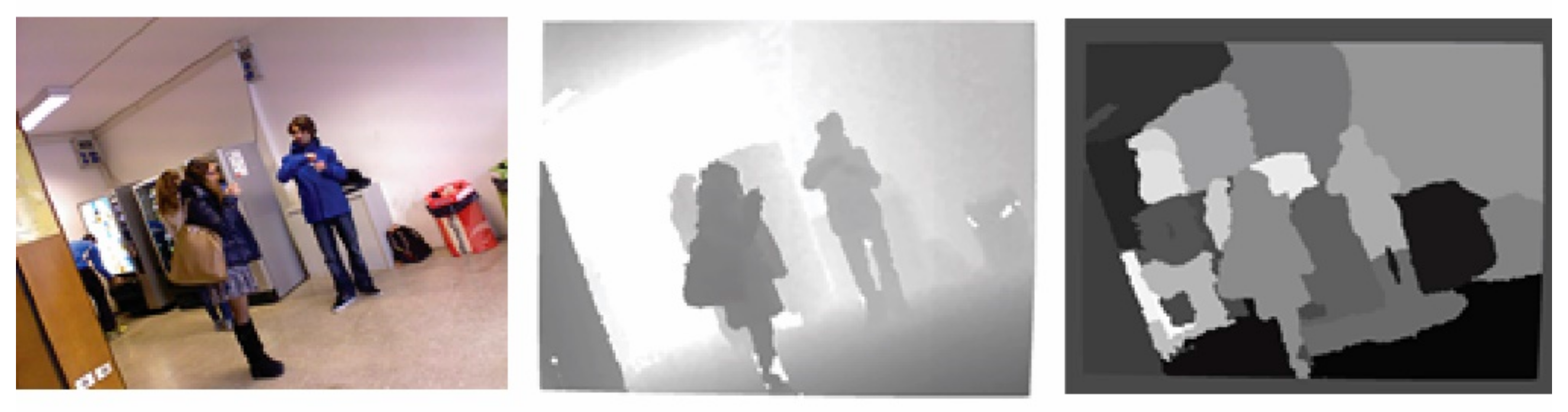
2.1. Depth Map Alignment and Segmentation
2.2. Face Detectors
2.2.1. VJ
2.2.2. SN
2.2.3. FL
2.2.4. RF
2.2.5. NPD
2.3. Filtering Steps
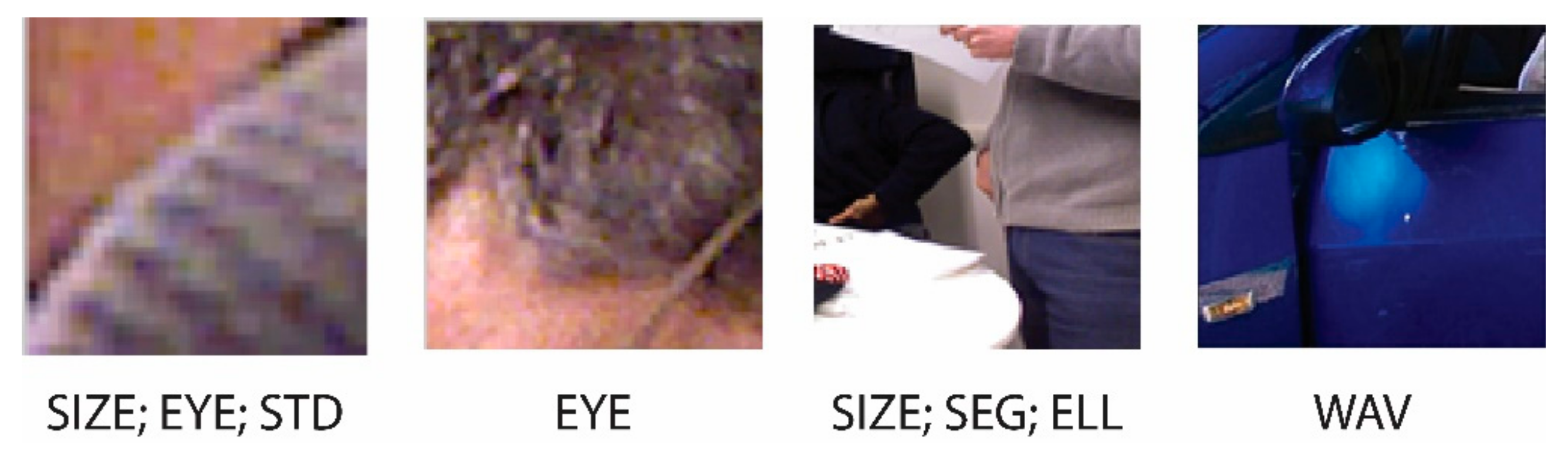
2.3.1. Image Size Filter (SIZE)
2.3.2. Flatness/Unevenness Filter (STD)
2.3.3. Segmentation-Based Filtering (SEG and ELL)
2.3.4. Eye-Based Filtering (EYE)
2.3.5. Filtering Based on the Analysis of the Depth Values (SEC)
2.3.6. WAV
3. Results and Discussion
3.1. Datasets
3.2. Performance Indicators
- Detection rate (DR): the ratio between the number of faces correctly detected and the total number of faces in the dataset. The faces were manually labeled. DR is evaluated at different precision levels considering different values of “eye distance”. Let be the Euclidean distance between the manually extracted and the detected left (right) eye positions. The relative error of detection is defined as , where the normalization factor is the Euclidean distance of the expected eye centers used to make the measurement independent of the scale of the face in the image and of the image size. There is a general agreement [56] that ED ≤ 0.25 is a good criterion for claiming eye detection, since this value roughly corresponds to an eye distance smaller than the eye width. Some face detectors (i.e., FL and RF) give the positions of the eye centers as the output, whereas for others (i.e., VJ and SN), the eye position is assumed to be a fixed position inside the face bounding box.
- False positives (FP): the number of candidate faces that do not include a face.
3.3. Experiments
4. Conclusions
Author Contributions
Funding
Conflicts of Interest
References
- Zeng, Z.; Pantic, M.; Roisman, G.I.; Huang, T.S. A Survey of Affect Recognition Methods: Audio, Visual, and Spontaneous Expressions. IEEE Trans. Pattern Anal. Mach. Intell. 2009, 31, 39–58. [Google Scholar] [CrossRef] [PubMed]
- Zhu, X.; Liu, X.; Lei, Z.; Li, S.Z. Face Alignment in Full Pose Range: A 3D Total Solution. IEEE Trans. Pattern Anal. Mach. Intell. 2019, 41, 78–92. [Google Scholar] [CrossRef] [PubMed]
- Xiong, X.; Torre, F.D. Supervised Descent Method and Its Applications to Face Alignment. In Proceedings of the 2013 IEEE Conference on Computer Vision and Pattern Recognition, Washington, DC, USA, 23–28 June 2013; pp. 532–539. [Google Scholar]
- Xie, X.; Jones, M.W.; Tam, G.K.L. Deep face recognition. In British Machine Vision Conference (BMVC); Xie, X., Jones, M.W., Tam, G.K.L., Eds.; BMVA Press: Durham, UK, 2015; pp. 41.1–41.12. [Google Scholar]
- Schroff, F.; Kalenichenko, D.; Philbin, J. FaceNet: A unified embedding for face recognition and clustering. In Proceedings of the 2015 IEEE Conference on Computer Vision and Pattern Recognition (CVPR), Boston, MA, USA, 7–12 June 2015; pp. 815–823. [Google Scholar]
- Taigman, Y.; Yang, M.; Ranzato, M.A.; Yang, M.; Wolf, L. DeepFace: Closing the Gap to Human-Level Performance in Face Verification. In Proceedings of the 2014 IEEE Conference on Computer Vision and Pattern Recognition, Columbus, OH, USA, 23–28 June 2014; pp. 1701–1708. [Google Scholar]
- Zhu, X.; Lei, Z.; Yan, J.; Yi, D.; Li, S.Z. High-fidelity Pose and Expression Normalization for face recognition in the wild. In Proceedings of the 2015 IEEE Conference on Computer Vision and Pattern Recognition (CVPR), Boston, MA, USA, 7–12 June 2015; pp. 787–796. [Google Scholar]
- Kim, M.; Kumar, S.; Pavlovic, V.; Rowley, H.A. Face tracking and recognition with visual constraints in real-world videos. In Proceedings of the 2008 IEEE Conference on Computer Vision and Pattern Recognition, Anchorage, AK, USA, 24–26 June 2008; pp. 1–8. [Google Scholar]
- Nanni, L.; Lumini, A.; Minto, L.; Zanuttigh, P. Face detection coupling texture, color and depth data. In Advances in Face Detection and Facial Image Analysis; Kawulok, M., Celebi, M., Smolka, B., Eds.; Springer: Cham, Switzerland, 2016; pp. 13–33. [Google Scholar]
- Nanni, L.; Lumini, A.; Dominio, F.; Zanuttigh, P. Effective and precise face detection based on color and depth data. Appl. Comput. Inform. 2014, 10, 1–13. [Google Scholar] [CrossRef]
- Zhang, C.; Zhang, Z. A Survey of Recent Advances in Face Detection; Microsoft: Redmond, WA, USA, 2010. [Google Scholar]
- Yang, M.H.; Kriegman, D.J.; Ahuja, N. Detecting faces in images: A survey. IEEE Trans. Pattern Anal. Mach. Intell. 2002, 24, 34–58. [Google Scholar] [CrossRef]
- Jin, H.; Liu, Q.; Lu, H. Face detection using one-class-based support vectors. In Proceedings of the Sixth IEEE International Conference on Automatic Face and Gesture Recognition, Seoul, Korea, 19 May 2004; pp. 457–462. [Google Scholar]
- Viola, P.A.; Jones, M.P. Rapid object detection using a boosted cascade of simple features. In Proceedings of the 2001 IEEE Computer Society Conference on Computer Vision and Pattern Recognition (CVPR), Kauai, HI, USA, 8–14 December 2001; p. 3. [Google Scholar]
- Li, J.; Zhang, Y. Learning SURF Cascade for Fast and Accurate Object Detection. In Proceedings of the 2013 IEEE Conference on Computer Vision and Pattern Recognition, Washington, DC, USA, 23–28 June 2013; pp. 3468–3475. [Google Scholar]
- Jain, V.; Learned-Miller, E. FDDB: A Benchmark for Face Detection in Unconstrained Setting; University of Massachusetts: Amherst, MA, USA, 2010. [Google Scholar]
- Cheney, J.; Klein, B.; Klein, A.K.; Klare, B.F. Unconstrained Face Detection: State of the Art Baseline and Challenges. In Proceedings of the 8th IAPR International Conference on Biometrics (ICB), Phuket, Thailand, 19–22 May 2015. [Google Scholar]
- Lienhart, R.; Maydt, J. An extended set of Haar-like features for rapid object detection. In Proceedings of the International Conference on Image Processing, Rochester, NY, USA, 22–25 September 2002; pp. I-900–I-903. [Google Scholar]
- Huang, C.; Ai, H.; Li, Y.; Lao, S. Learning sparse features in granular space for multi-view face detection. In Proceedings of the 7th International Conference on Automatic Face and Gesture Recognition (FGR06), Southampton, UK, 10–12 April 2006; pp. 401–406. [Google Scholar]
- Pham, M.T.; Gao, Y.; Hoang, V.D.; Hoang, V.D.; Cham, T.J. Fast polygonal integration and its application in extending haar-like features to improve object detection. In Proceedings of the CVPR, IEEE Computer Society Conference on Computer Vision and Pattern Recognition, San Francisco, CA, USA, 13–18 June 2010. [Google Scholar]
- Jin, H.; Liu, Q.; Lu, H.; Tong, X. Face detection using improved LBP under bayesian framework. In Proceedings of the International Conference on Image and Graphics, Hong Kong, China, 18–20 December 2004; pp. 306–309. [Google Scholar]
- Zhang, H.; Gao, W.; Chen, X.; Zhao, D. Object detection using spatial histogram features. Image Vis. Comput. 2006, 24, 327–341. [Google Scholar] [CrossRef]
- Zhu, Q.; Yeh, M.C.; Cheng, K.T.; Avidan, S. Fast Human Detection Using a Cascade of Histograms of Oriented Gradients. In Proceedings of the 2006 IEEE Computer Society Conference on Computer Vision and Pattern Recognition, New York, NY, USA, 17–22 June 2006; Volume 2, pp. 1491–1498. [Google Scholar]
- Jianguo, L.; Tao, W.; Yimin, Z. Face detection using SURF cascade. In Proceedings of the 2011 IEEE International Conference on Computer Vision Workshops (ICCV Workshops), Barcelona, Spain, 6–13 November 2011; pp. 2183–2190. [Google Scholar]
- Bin, Y.; Yan, J.; Lei, Z.; Li, S.Z. Aggregate channel features for multi-view face detection. In Proceedings of the IEEE International Joint Conference on Biometrics, Clearwater, FL, USA, 29 September–2 October 2014; pp. 1–8. [Google Scholar]
- Brubaker, S.C.; Wu, J.; Sun, J.; Mullin, M.D.; Rehg, J.M. On the design of cascades of boosted ensembles for face detection. Int. J. Comput. Vis. 2008, 77, 65–86. [Google Scholar] [CrossRef]
- Pham, M.T.; Cham, T.J. Fast training and selection of haar features during statistics in boosting-based face detection. In Proceedings of the CVPR, IEEE Computer Society Conference on Computer Vision and Pattern Recognition, Rio de Janeiro, Brazil, 14–21 October 2007. [Google Scholar]
- Küblbeck, C.; Ernst, A. Face detection and tracking in video sequences using the modifiedcensus transformation. Image Vis. Comput. 2006, 24, 564–572. [Google Scholar] [CrossRef]
- Huang, C.; Ai, H.; Li, Y.; Lao, S. High-Performance Rotation Invariant Multiview Face Detection. IEEE Trans. Pattern Anal. Mach. Intell. 2007, 29, 671–686. [Google Scholar] [CrossRef]
- Mathias, M.; Benenson, R.; Pedersoli, M.; Gool, L.V. Face Detection without Bells and Whistles. In ECCV; Springer: Cham, Switzerland, 2014. [Google Scholar]
- Nilsson, M.; Nordberg, J.; Claesson, I. Face Detection using Local SMQT Features and Split up Snow Classifier. In Proceedings of the 2007 IEEE International Conference on Acoustics, Speech and Signal Processing-ICASSP ’07, Honolulu, HI, USA, 15–20 April 2007; pp. II-589–II-592. [Google Scholar]
- Asthana, A.; Zafeiriou, S.; Cheng, S.; Pantic, M. Robust Discriminative Response Map Fitting with Constrained Local Models, CVPR; IEEE: Portland, OR, USA, 2013. [Google Scholar]
- Liao, S.; Jain, A.K.; Li, S.Z. A Fast and Accurate Unconstrained Face Detector. IEEE Trans. Pattern Anal. Mach. Intell. 2016, 38, 211–223. [Google Scholar] [CrossRef]
- Markuš, N.; Frljak, M.; Pandžić, I.S.; Ahlberg, J.; Forchheimer, R. Fast Localization of Facial Landmark Points. arXiv 2014, arXiv:1403.6888. [Google Scholar]
- Li, H.; Lin, Z.L.; Shen, X.; Brandt, J.; Hua, G. A convolutional neural network cascade for face detection. In Proceedings of the 2015 IEEE Conference on Computer Vision and Pattern Recognition (CVPR), Boston, MA, USA, 7–12 June 2015; pp. 5325–5334. [Google Scholar]
- Girshick, R.; Donahue, J.; Darrell, T.; Malik, J. Rich Feature Hierarchies for Accurate Object Detection and Semantic Segmentation. In Proceedings of the 2014 IEEE Conference on Computer Vision and Pattern Recognition, Columbus, OH, USA, 23–28 June 2014; pp. 580–587. [Google Scholar]
- Farfade, S.S.; Saberian, M.; Li, L.J. Multi-View Face Detection Using Deep Convolutional Neural Networks; Cornell University: Ithaca, NY, USA, 2015. [Google Scholar]
- Yang, W.; Zhou, L.; Li, T.; Wang, H. A Face Detection Method Based on Cascade Convolutional Neural Network. Multimed. Tools Appl. 2018, 78, 1–18. [Google Scholar] [CrossRef]
- Zhang, S.; Zhu, X.; Lei, Z.; Shi, H.; Wang, X.; Li, S.Z. S^3FD: Single Shot Scale-Invariant Face Detector. In Proceedings of the 2017 IEEE International Conference on Computer Vision (ICCV), Venice, Italy, 22–29 October 2017; pp. 192–201. [Google Scholar]
- Yang, B.; Yan, J.; Lei, Z.; Li, S.Z. Convolutional Channel Features. In Proceedings of the 2015 IEEE International Conference on Computer Vision (ICCV), Boston, MA, USA, 7–13 December 2015; pp. 82–90. [Google Scholar]
- Zhang, K.; Zhang, Z.; Li, Z.; Qiao, Y. Joint Face Detection and Alignment Using Multitask Cascaded Convolutional Networks. IEEE Signal Process. Lett. 2016, 23, 1499–1503. [Google Scholar] [CrossRef]
- Faltemier, T.C.; Bowyer, K.W.; Flynn, P.J. Using a Multi-Instance Enrollment Representation to Improve 3D Face Recognition. In Proceedings of the 2007 First IEEE International Conference on Biometrics: Theory, Applications, and Systems, Crystal City, VA, USA, 27–29 September 2007; pp. 1–6. [Google Scholar]
- Gupta, S.; Castleman, K.R.; Markey, M.K.; Bovik, A.C. Texas 3D Face Recognition Database. In Proceedings of the IEEE Southwest Symposium on Image Analysis and Interpretation, Austin, TX, USA, 23–25 May 2010; pp. 97–100. [Google Scholar]
- Min, R.; Kose, N.; Dugelay, J. KinectFaceDB: A Kinect Database for Face Recognition. IEEE Trans. Syst. Man Cybern. Syst. 2014, 44, 1534–1548. [Google Scholar] [CrossRef]
- Guo, Y.; Sohel, F.A.; Bennamoun, M.; Wan, J.; Lu, M. RoPS: A local feature descriptor for 3D rigid objects based on rotational projection statistics. In Proceedings of the 2013 1st International Conference on Communications, Signal Processing, and their Applications (ICCSPA), Sharjah, UAE, 12–14 February 2013; pp. 1–6. [Google Scholar]
- Zhou, S.; Xiao, S. 3D face recognition: A survey. Hum. Cent. Comput. Inf. Sci. 2018, 8, 35. [Google Scholar] [CrossRef]
- Hg, R.I.; Jasek, P.; Rofidal, C.; Nasrollahi, K.; Moeslund, T.B.; Tranchet, G. An RGB-D Database Using Microsoft’s Kinect for Windows for Face Detection. In Proceedings of the 2012 Eighth International Conference on Signal Image Technology and Internet Based Systems, Naples, Italy, 25–29 November 2012; pp. 42–46. [Google Scholar]
- Dixon, M.; Heckel, F.; Pless, R.; Smart, W.D. Faster and more accurate face detection on mobile robots using geometric constraints. In Proceedings of the 2007 IEEE/RSJ International Conference on Intelligent Robots and Systems, San Diego, CA, USA, 29 October–2 November 2007; pp. 1041–1046. [Google Scholar]
- Burgin, W.; Pantofaru, C.; Smart, W.D. Using depth information to improve face detection. In Proceedings of the 6th International Conference on Human-Robot Interaction, Lausanne, Switzerland, 8–11 March 2011; pp. 119–120. [Google Scholar]
- Shieh, M.Y.; Hsieh, T.M. Fast Facial Detection by Depth Map Analysis. Math. Probl. Eng. 2013, 2013, 1–10. [Google Scholar] [CrossRef]
- Shotton, J.; Sharp, T.; Kipman, A.; Fitzgibbon, A.; Finocchio, M.; Blake, A.; Cook, M.; Moore, R. Real-time human pose recognition in parts from single depth images. Commun. ACM 2013, 56, 116–124. [Google Scholar] [CrossRef]
- Mattheij, R.; Postma, E.; Van den Hurk, Y.; Spronck, P. Depth-based detection using Haarlike features. In Proceedings of the BNAIC 2012 Conference, Maastricht, The Netherlands, 25–26 October 2012; pp. 162–169. [Google Scholar]
- Jiang, F.; Fischer, M.; Ekenel, H.K.; Shi, B.E. Combining texture and stereo disparity cues for real-time face detection. Signal Process. Image Commun. 2013, 28, 1100–1113. [Google Scholar] [CrossRef]
- Anisetti, M.; Bellandi, V.; Damiani, E.; Arnone, L.; Rat, B. A3fd: Accurate 3d face detection. In Signal Processing for Image Enhancement and Multimedia Processing; Damiani, E., Dipanda, A., Yetongnon, K., Legrand, L., Schelkens, P., Chbeir, R., Eds.; Springer: Boston, MA, USA, 2008; pp. 155–165. [Google Scholar]
- Huang, G.B.; Ramesh, M.; Berg, T.; Learned-Miller, E. Labeled Faces in the Wild: A Database for Studying Face Recognition in Unconstrained Environments; University of Massachusetts: Amherst, MA, USA, 2007. [Google Scholar]
- Jesorsky, O.; Kirchberg, K.J.; Frischholz, R. Robust Face Detection Using the Hausdorff Distance. In AVBPA; Springer: Berlin/Heidelberg, Germany, 2001. [Google Scholar]
- Herrera, D.C.; Kannala, J.; Heikkilä, J. Joint Depth and Color Camera Calibration with Distortion Correction. IEEE Trans. Pattern Anal. Mach. Intell. 2012, 34, 2058–2064. [Google Scholar] [CrossRef]
- Mutto, C.D.; Zanuttigh, P.; Cortelazzo, G.M. Fusion of Geometry and Color Information for Scene Segmentation. IEEE J. Sel. Top. Signal Process. 2012, 6, 505–521. [Google Scholar] [CrossRef]
- Comaniciu, D.; Meer, P. Mean shift: A robust approach toward feature space analysis. IEEE Trans. Pattern Anal. Mach. Intell. 2002, 24, 603–619. [Google Scholar] [CrossRef]
- Friedman, J.; Hastie, T.; Tibshirani, R. Additive logistic regression: A statistical view of boosting. Ann. Stat. 2000, 38, 337–374. [Google Scholar] [CrossRef]
- Gal, O. Fit_Ellipse. Available online: https://www.mathworks.com/matlabcentral/fileexchange/3215-fit_ellipse (accessed on 2 October 2003).
- Tan, X.; Song, S.; Zhou, Z.H.; Chen, S. Enhanced pictorial structures for precise eye localization under uncontrolled conditions. In Proceedings of the IEEE Computer Society Conference on Computer Vision and Pattern Recognition (CVPR’09), Miami, FL, USA, 20–25 June 2009; pp. 1621–1628. [Google Scholar]
- Skodras, E.; Fakotakis, N. Precise localization of eye centers in low resolution color images. Image Vis. Comput. 2015, 36, 51–60. [Google Scholar] [CrossRef]
- Kovesi, P. Image features from Phase Congruency. J. Comput. Vis. Res. 1999, 1, 1–27. [Google Scholar]
- Bobulski, J. Wavelet transform in face recognition. In Biometrics, Computer Security Systems and Artificial Intelligence Applications; Saeed, K., Pejaś, J., Mosdorf, R., Eds.; Springer Science + Business Media: New York, NY, USA, 2006; pp. 23–29. [Google Scholar]
- Ren, Z.; Meng, J.; Yuan, J. Depth camera based hand gesture recognition and its applications in Human-Computer-Interaction. In Proceedings of the 2011 8th International Conference on Information, Communications & Signal Processing, Singapore, 13–16 December 2011; pp. 1–5. [Google Scholar]
- Dominio, F.; Donadeo, M.; Zanuttigh, P. Combining multiple depth-based descriptors for hand gesture recognition. Pattern Recognit. Lett. 2014, 50, 101–111. [Google Scholar] [CrossRef]


| Dataset | Number Images | Color Resolution | Depth Resolution | Number Faces | Difficulty Level |
|---|---|---|---|---|---|
| MHG | 42 | 640 × 480 | 640 × 480 | 42 | Low |
| PHG | 59 | 1280 × 1024 | 640 × 480 | 59 | Low |
| PFD | 132 | 1280 × 1024 | 640 × 480 | 150 | High |
| PFD2 | 316 | 1920 × 1080 | 512 × 424 | 363 | High |
| MERGED | 549 | --- | --- | 614 | High |
| BioID | 1521 | 384 × 286 | --- | 1521 | High |
| Face Detector(s)/Ensemble | +Poses | DR | FP |
|---|---|---|---|
| VJ(2) | No | 55.37 | 2528 |
| RF(−1) | No | 47.39 | 4682 |
| RF(−0.8) | No | 47.07 | 3249 |
| RF(−0.65) | No | 46.42 | 1146 |
| SN(1) | No | 66.61 | 508 |
| SN(10) | No | 46.74 | 31 |
| FL | No | 78.18 | 344 |
| NPD | No | 55.70 | 1439 |
| SFD | No | 81.27 | 186 |
| VJ(2) * | Yes | 65.31 | 6287 |
| RF(−1) * | Yes | 49.67 | 19,475 |
| RF(−0.8) * | Yes | 49.67 | 14,121 |
| RF(−0.65) * | Yes | 49.02 | 5895 |
| SN(1) * | Yes | 74.59 | 1635 |
| SN(10) * | Yes | 50.16 | 48 |
| FL * | Yes | 83.39 | 891 |
| NPD * | Yes | 64.17 | 10,431 |
| FL + RF(−0.65) | No | 83.06 | 1490 |
| FL + RF(−0.65) + SN(1) | No | 86.16 | 1998 |
| FL + RF(−0.65) + SN(1) * | Mixed | 88.44 | 3125 |
| FL * + SN(1) * | Yes | 87.79 | 2526 |
| FL * + RF(−0.65) + SN(1) * | Mixed | 90.39 | 3672 |
| FL * + RF(−0.65) + SN(1) * + SFD | Mixed | 91.21 | 3858 |
| FL * + RF(−0.65) + SN(1) * + NPD * + SFD | Mixed | 92.02 | 16,325 |
| Face Detector(s)/Ensemble | +Poses | DR (ED < 0.15) | DR (ED < 0.25) | DR (ED < 0.35) | (FP) |
|---|---|---|---|---|---|
| VJ(2) | No | 13.08 | 86.46 | 99.15 | 517 |
| RF(−1) | No | 87.84 | 98.82 | 99.08 | 80 |
| RF(−0.8) | No | 87.84 | 98.82 | 99.08 | 32 |
| RF(−0.65) | No | 87.84 | 98.82 | 99.08 | 21 |
| SN(1) | No | 71.27 | 96.38 | 97.76 | 12 |
| SN(10) | No | 72.06 | 98.16 | 99.74 | 172 |
| FL | No | 92.57 | 94.61 | 94.67 | 67 |
| SFD | No | 99.21 | 99.34 | 99.34 | 1 |
| VJ(2) * | Yes | 13.08 | 86.46 | 99.15 | 1745 |
| RF(−1) * | Yes | 90.53 | 99.15 | 99.41 | 1316 |
| RF(−0.8) * | Yes | 90.53 | 99.15 | 99.41 | 589 |
| RF(−0.65) * | Yes | 90.53 | 99.15 | 99.41 | 331 |
| SN(1) * | Yes | 71.33 | 96.52 | 97.90 | 193 |
| SN(10) * | Yes | 72.12 | 98.36 | 99.87 | 1361 |
| FL * | Yes | 92.57 | 94.61 | 94.67 | 1210 |
| FL + RF(−0.65) | No | 98.42 | 99.74 | 99.74 | 88 |
| FL + RF(−0.65) + SN(10) | No | 99.15 | 99.93 | 99.93 | 100 |
| FL + RF(−0.65) + SN(1) * | Mixed | 99.15 | 100 | 100 | 281 |
| FL * + SN(1) * | Yes | 98.03 | 99.87 | 99.93 | 260 |
| FL * + RF(−0.65) + SN(1) * | Mixed | 99.15 | 100 | 100 | 1424 |
| FL * + RF(−0.65) + SN(1) * + SFD | Mixed | 99.41 | 100 | 100 | 1425 |
| Filter Combination | DR | FP |
|---|---|---|
| SIZE | 91.21 | 1547 |
| SIZE + STD | 91.21 | 1514 |
| SIZE + STD + SEG | 91.21 | 1485 |
| SIZE + STD + SEG + ELL | 91.04 | 1440 |
| SIZE + STD + SEG + ELL + EYE | 90.55 | 1163 |
| SIZE + STD + SEG + ELL + SEC + EYE | 90.39 | 1132 |
| SIZE + STD + SEG + ELL + SEC + EYE + WAV | 90.07 | 1018 |
| Detection Method/Filter | ms |
|---|---|
| RF | 12,571 |
| SN | 1371 |
| FL | 170 |
| SPD | 175 |
| SIZE | 0.33 |
| STD | 10.86 |
| SEG | 8.808 |
| ELL | 10.24 |
| EYE | 19,143 |
| WAV | 179.4 |
© 2019 by the authors. Licensee MDPI, Basel, Switzerland. This article is an open access article distributed under the terms and conditions of the Creative Commons Attribution (CC BY) license (http://creativecommons.org/licenses/by/4.0/).
Share and Cite
Nanni, L.; Brahnam, S.; Lumini, A. Face Detection Ensemble with Methods Using Depth Information to Filter False Positives. Sensors 2019, 19, 5242. https://doi.org/10.3390/s19235242
Nanni L, Brahnam S, Lumini A. Face Detection Ensemble with Methods Using Depth Information to Filter False Positives. Sensors. 2019; 19(23):5242. https://doi.org/10.3390/s19235242
Chicago/Turabian StyleNanni, Loris, Sheryl Brahnam, and Alessandra Lumini. 2019. "Face Detection Ensemble with Methods Using Depth Information to Filter False Positives" Sensors 19, no. 23: 5242. https://doi.org/10.3390/s19235242
APA StyleNanni, L., Brahnam, S., & Lumini, A. (2019). Face Detection Ensemble with Methods Using Depth Information to Filter False Positives. Sensors, 19(23), 5242. https://doi.org/10.3390/s19235242