1. Introduction
Retinal fundus images provide a key insight into the various entities within the human retina. Any abnormal changes in these features point towards the type and seriousness of numerous eye diseases such as Diabetic Retinopathy (DR) and Diabetic Maculopathy (DM), both of which are main contributors towards global blindness. These diseases stealthily manifest themselves, and are usually not diagnosed until they have progressed to more advanced stages where their treatment becomes both costly and ineffective. One of the dominating feature in fundus images is the vessel tree structure, referred to as vasculature. Therefore, accurate detection of vaculature is the primary step as its detection acts as a reliable biomarker towards classification of both the retinal features and any associated pathologies [
1].
Recent advancements in medical imaging technology have guided the scientists in the image processing community to focus on analyzing these medical images so as to mimic the diagnostic process of a medical professional. The computerized analysis of bio-medical images has found numerous uses in different medicinal applications ranging from diagnosis, progression monitoring, and treatment. Every passing day sees advances in digital image processing with expansion in both efficiency and the precision of such methods [
2]. The data in bio-medical images is generally unbalanced (disease appears in small percentage of dataset) [
3,
4], unstable (variations in surface response due to uneven illumination) [
5], and characterized by a high degree of complexity [
3]. In this kind of a scenario, automated extraction of bio-markers in medical images exhibits great potential towards exploiting big data analytics in improving medical practice, and synchronization of diagnosis and prognosis conventions.
A broken bone, for example, is visible through an X-Ray, so researchers have aimed at developing an adaptive threshold that can detect the abnormality intelligently without any human supervision. Detecting retinal features and any associated pathologies is a bit more subtle than X-Rays. Over time, numerous highly sophisticated adaptive filtering techniques have surfaced that can almost match the human expert in the detection of these anomalies. The knowledge gap is still vast in terms of both detection and validation of these complex-shaped pathologies that result in numerous eye diseases every year.
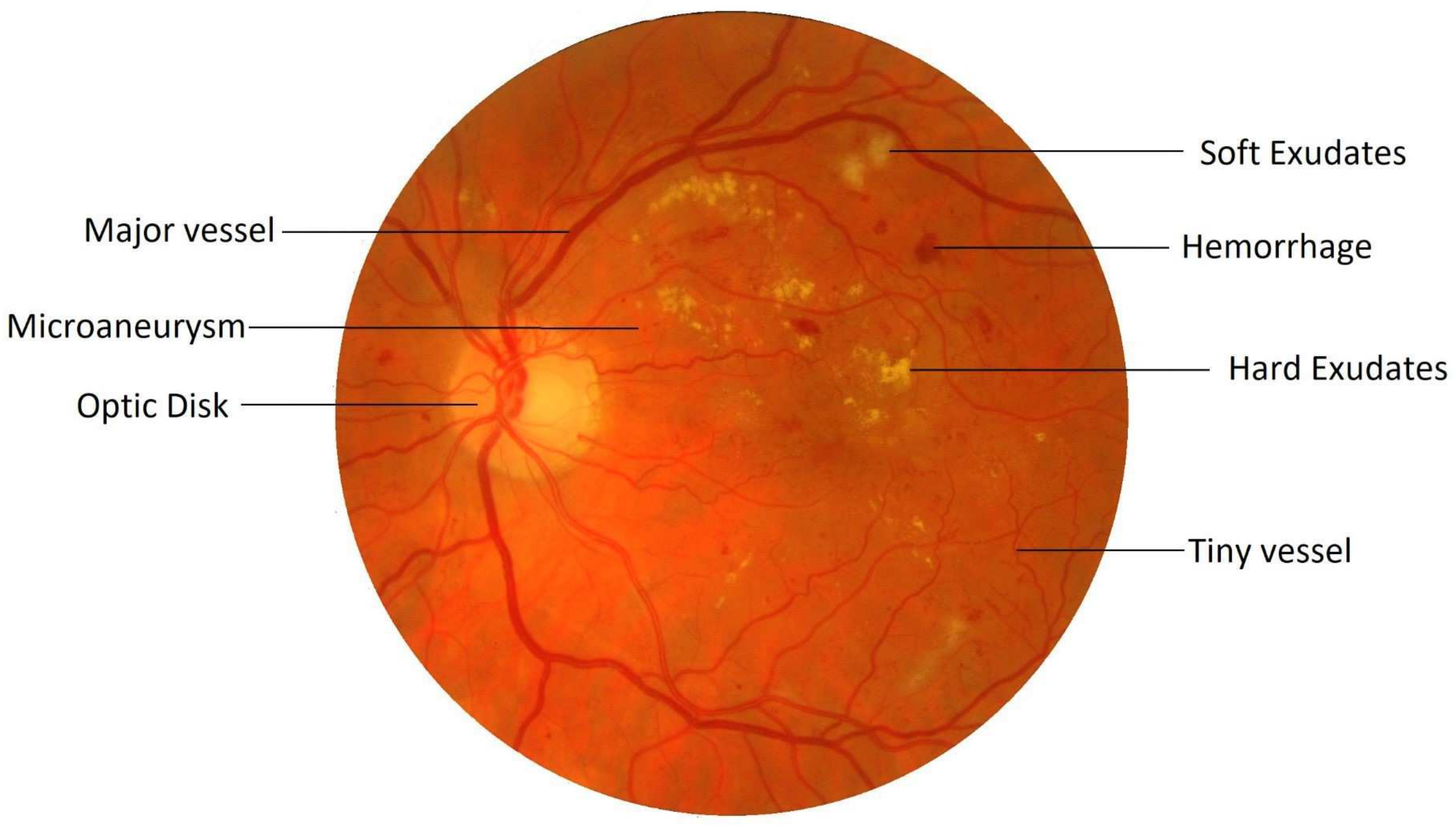
Retinal image processing has attracted tremendous research focus over the years with varying degrees of success. Demarcation of the retinal vessel structure by a human expert is both time-consuming and tedious, thereby augmenting the need for automation of this crucial task to enable mass screenings. Pointing out troublesome features in the retina is a difficult task. For most of the other diseases, predefined lesion patterns help determine with conviction the presence or absence of a disease like cancer. However, DR is different as there can be multiple forms of anomalies associated with it, such as Microaneurysms, Exudates, and Neovascularization, etc., as shown in
Figure 1. Each of these types is treated as a separate problem for detection and overall diagnosis. Then, the results from the integration of their outputs constitute the pathology detections in the image.
Automated vessel mapping of the retina is hindered by many factors, such as variations in the shapes, sizes, and direction of the dense vascular network present within the retina. Also, the enhancement of these blood vessels alongside the suppression of background information, plays an important role in increasing the accuracy of such a vessel mapping regimen. During the process of segmentation, all the existing morphological detectors tend to act poorly on vessels of varying sizes. The segmentation process becomes increasingly prone to error, particularly during the binarization phase, due to the changing orientation of vessels and poor contrast among them. Line detectors are one similar form of morphological detectors which have been employed for vessel detection in retinal images.
A basic or fixed-length line detector is based on establishing a correlation with the vessel geometry. A preset line segment is laid over a set of pixels, and a high matched response suggests the presence of a linear structure, or in this case, a vessel. Although line detectors are very efficient at detecting the presence of vessels, they fail to achieve an accurate segmentation due to the choice of length of the line detector. Detectors of smaller lengths or scales tend to produce shadows around vessel regions, and filters of larger length generate fake extensions at vessel endpoints. As there was a strict trade-off between these, this led to the evolution of multi-scale line detectors, which combines the responses of different scales while countering their adverse effects.
A multi-scale line detector identifies vascular structures in an image by iteratively rotating the detector at a pixel to capture the vessels at different angles at that point. With the rotation along some predefined angles, another critical parameter is the choice of detector’s variation in scale, which hunts for corresponding features of comparable lengths. However, this method of using multi-scale detectors had its own set of problems. This detector operates in all directions, and the efficacy of feature extraction in any specific direction is co-variant with the contrast of those features. While scanning multiple angles for the presence of vessels, the vessel features with high contrast dominate those with lower contrast. This results in the highlighting of certain vessel pixels and suppression of others to the extent that, tiny vessels, particularly at the endpoints of the vascular map, are usually the most affected. The tiny vessels are not the only victims to this problem, as the reconstruction of edges of the larger vessels are also affected during the combined binarization process.
To tackle these problems, we propose a three-pronged strategy with a new directional multi-scale line detector that, instead of scanning multiple angles within the whole image, focuses on a fixed direction while scanning a narrow angular range. Such a direction-specific filter will still be burdened by an image having multi-orientation features, thereby causing a loss in the sensitivity indicator. The second prong of this strategy lies in the use of directional images instead of the original image, having only those features or vessels which fall in line with the direction of the angular detector. This strategy is adopted with the expectation that, an image having only directional information will help boost the performance of the angle-specific detector while significantly reducing the false-positives.
Towards the end, a novel binarization technique based on the standard deviation of the directional line filter is used to eliminate the false extensions introduced by the larger-scale line filters. All the resultant features evolved from different directions, are recombined to yield the overall retinal vessel map. Therefore, directional segmentation and binarization of target features produces significantly improved results, as the detector becomes more immune to the omni-directional present in the input image. The proposed method is also notably faster as sensitivity, specificity, and accuracy of the vessel segmentation are enhanced without the use of any denoiser or advanced thresholding techniques such as region growing or overlaying.
The remaining portion of this paper is organized as follows:
Section 2 summarizes the related work followed by
Section 3, describing each step of the proposed technique in detail.
Section 4 contains the experimental results elaborating the tested retinal image databases, algorithm’s performance judging criteria, and comparison with state-of-the-art techniques.
Section 5 concludes the paper by discussing the key findings of this study, followed by recommendations for potential future research work.
2. Literature Review
Pointing out the features and troublesome lesions in the retina is a challenging task. Many research groups around the globe have been studying techniques to help determine these retinal features, and to maximize progress and collaboration, it has been turned into international competitions such as the STructured Analysis of the Retina (STARE) [
6] and Digital Retinal Images for Vessel Extraction (DRIVE) [
7] databases, etc. Many algorithms have surfaced that although not being applied in clinical practice yet, have provided unique insights into the solution of the problem at hand. A usual concern with any automated system is the accuracy and precision of the data it learns from. So, retinal images with all their differences in vessel size, contrast, presence of pathologies, and noisy vessel boundary problems make vascular segmentation an increasingly daunting task.
The vessel detection approaches using image processing, are categorized as either supervised or unsupervised learning techniques. Supervised methods identify the vessel pixels based on machine learning algorithms that use expert-marked ground truth samples to train a classifier. Unsupervised methods are the more popular choice, as they require no such pre-labeled training data and patterns of blood vessels hard-coded into the algorithm’s structure to obtain accurate segmentation.
2.1. Supervised Learning Methods
These techniques require a set of training data and relevant feature extraction followed by classification for vessel segmentation. First of all, constraints such as a viable training set (manually labeled into foreground and background), and the number of training data sets available, dictate the efficiency of the classification. Secondly, a feature index is created that helps differentiate between the vessel and non-vessel pixels which are later utilized by the classifier for the overall segmentation of vessels. The requirement of training data, large feature index and considerable classifier training time are the main drawbacks of supervised methods. On the other hand, ample training data coupled with a powerful classifier can lead to a significantly accurate segmentation of blood vessels.
Niemeijer et al. [
8] used a multi-scale Gaussian feature vector followed by a K-Nearest-Neighbors (KNN) classifier for supervised vessel segmentation. Staal et al. [
7] built a feature set evolved from 27 different attributes using the abstraction of image ridges, and fed them to a KNN classifier for calculating the probability of a pixel being a vessel entity. Ricci and Perfetti [
9] used two orthogonal line operators and SVM on the green channel of retinal images to improve the accuracy and Area Under the Curve (AUC) parameters of their method. They reduced the false-positives and false-negatives by assignment of different weights to the errors of both categories, respectively. Marin et al. [
10] utilized a grey-level and moment invariants-based feature set to train a multi-layer Neural Network (NN) to differentiate between the vessel and non-vessel pixels. You et al. [
11] constructed a Support Vector Machine (SVM) and a feature vector by using radial projections from large and tiny vessels separately to recognize the retinal vasculature.
Fraz et al. [
12] used an ensemble classification-based technique relying on orientation and morphological analysis of vessels. A multi-scale Gabor filter helped extract these features and a decision tree classifier was used in this approach, but it failed to report any objective quality measures. Franklin et al. [
13] used all three-color planes of a fundus image to extract vessel features, eventually classifying through a multi-layer perceptron NN. Li et al. [
14] proposed a cross modality learning approach without involving any preprocessing steps to induce robustness towards the training set. Their method was tested on DRIVE, STARE and CHASE_DB1 datasets with excellent results for both normal and pathological retinal fundus images.
Orlando et al. [
15] used fully connected conditional random field method that worked with a structured SVM to achieve a high specificity score of 0.9870. They randomized the training process by taking random sample of pixels from different sets of images from the STARE dataset for efficient elongated structure segmentation through a machine learning approach. Dasgupta and Singh [
16] also employed a FCCN to segment the vessels as a multi-label inference task. They used CLAHE during the preprocessing stage followed by 7 CNN layers on only the DRIVE dataset, to achieve remarkable sensitivity and accuracy scores of 0.9691 and 0.9533, respectively.
Alom et al. [
17] used a Recurrent Residual Convolutional Neural Network (RRCNN) to take advantage of both residual and recurrent CNN for training deep architectures and better feature representation, respectively. They tested their technique on a wide variety of bio medical images including retinal fundus images with the same degree of efficiency. Oliveira et al. [
18] used multi-scale Fully Convolutional Neural Networks (FCNN) that employ varying angles and branching patterns of vessels as the basis for data augmentation and prognosis. The Stationary Wavelet Transform explores the vessel rotation information to give the multi-scale tortuosity features that help the learning phase during training to refine the vascular map.
Li et al. [
19] constructed a new DR dataset known as DDR, in which they compiled 13,673 retinal images from a wide variety of fundus imaging devices and hospitals across China. Many recent deep learning models were tested on this dataset to evaluate their efficacy in vessel and small lesion recognition. Li et al. [
20] employed a connection sensitive loss model along with a attention gate NN to improve the accuracy of vessel detection. Segmenting thin vessels and boundaries was made more efficient by concatenating attention weights to features as this method reported an accuracy of 0.9563 and 0.9673 for the DRIVE and STARE datasets, respectively.
Jiang et al. [
21] used extensive pre-processing and denoising for image cleanup, followed by a combined dilated convolution technique for data augmentation. A Deep Convolutional Neural Network (DCNN) was constructed with the use of skip layer connection during decoding, which helped their method achieve an impressive accuracy score of 0.9709. Guo et al. [
22] proposed the use of multi-level features through a multi-scale Deeply Supervised Network (DSN) to achieve high AUC scores on the DRIVE, STARE and CHASE_DB1 datasets. The method used deep supervision by information exchange among higher and lower level layers for better fusion result, leading to effective retinal vessel segmentation and noise suppression.
Considering the disadvantages of supervised learning methods, a set of pre-labeled data, significant training computation times and complex feature vectors reduce the overall system efficiency in a real-world scenario. Also, the features of interest must be manually fed to the classifier as compared to the unsupervised learning methods, where the features are acquired by the algorithm itself. This causes a problem when the classifier is presented with a feature it is not already trained for. Therefore, the system may put that feature in the wrong class, or in this case, label a vessel pixel as non-vessel and vice-versa.
2.2. Unsupervised Learning Methods
These methods try to identify features of interest based on the similarity criteria and intrinsic attributes, without the need for manual intervention. These methods owe their popularity in literature to the independence from training data and faster execution times and therefore, learning is limited or altogether absent. Vessel detection in unsupervised methods is done at individual pixel-level, and the complicated nature of retinal vascular map combined with the presence of noise and pathologies implies that reliable segmentation remains a challenging problem. Unsupervised methods are further categorized into five groups: morphological approaches, matched filtering algorithms, vessel tracking, multi-scale processes, and model-based techniques.
Miri and Mahloojifar [
23] presented the use of Fast Discrete Curvelet Transform (FDCT) alongside multidimensional morphological processing for retinal vasculature extraction. Vessel boundary was tediously revised utilizing a layered morphological system, where the wrongly detected boundaries were deleted during this revision process, allowing for efficient reconstruction of small and tiny vessels. Xu et al. [
24] used elongation-based morphological shape detectors of retinal vessels by employing a twin attribute system that used geometric morphology alongside connected-tree branching methods, resulting in prominent vessel contrast enhancement.
Moghimirad et al. [
25] proposed the detection of midpoints of a vessel through the weighted medialness 2-D functions, resulting in high accuracy figures for vessel radius evaluation in a broad range of noisy and pathological images. Nguyen et al. [
26] suggested multiscale line identification, relying upon varying the length of a fundamental line detector to extract a threshold vessel image. A localized thresholding filter was stated by Ravichandran et al. [
27] for detection of vessels built on the entropy of that region. Contrast Limited Adaptive Histogram Equalization (CLAHE) followed by Wiener filter was used to denoise the image followed by a 2-D Gabor filter for additional vasculature refinement.
Martínez-Pérez et al. [
28] employed Region Growing (RG) technique to populate a scale-space representation of varying contrast via derivatives. The first and second derivative predictors helped cater for the contrast variation in the input image, resulting in superior segmentation results. Sofka et al. [
29] segmented retinal vessels by developing a Likelihood Ratio Vesselness (LRV) value to assess the worth of matched filter responses. Kar S and Maity S [
30] exhibited superior accuracy figures by using Curvelet function based on Fuzzy C-Means (FCM) architecture to detect blood vessels and the Optic Disc (OD). Amin and Yan [
31] presented a robust vessel identification method in the form of sorted log-Gabor wavelets. The high paced wavelets exhibited noticeable immunity against the contrast and phase variations through a calibrated threshold.
Palomera-Pérez et al. [
32] suggested a collateral setup which used a single plane (horizontal) and blended plane (horizontal plus vertical) feature markers for the evaluation of information within the retinal images. This parallel setup allowed for faster and effective feature extraction, and RG based vascular segmentation with a high degree of accuracy. Cinsdikici and Aydin [
33] designed the combination of matched filtering with ANT colony algorithms to extract the entire vessel map. Some preprocessing followed by length sifting is utilized for vessel and capillary recognition, which became unproductive in cases with pathology.
Zhang et al. [
34] used wavelet transform to convert standard images into 3D rotating orientation scores, which were further refined by multi-scale second-order Gaussian derivatives. This method was tested on six different retinal datasets and showed competitive results, especially with difficult cases like vessel crossings. Neto et al. [
35] aimed to tackle the central vessel reflex by Gaussian smoothing and top-hat transformation. A curvature analysis followed by adaptive local thresholding resulted in excellent all-round performance parameters on both DRIVE and STARE datasets. Karn et al. [
36] constructed a hybrid active contour model based on a Gradient Vector Flow (GVF) framework to focus on tiny blood vessels. A novel preprocessing technique coupled with phase-based binarization helped this method report high accuracy scores and effective vessel segmentation.
Aguirre et al. [
37] utilized the removal of the OD and low-pass radius filter in preprocessing before employing a 30-element Gabor filter for vessel segmentation. Morphology-based decision rules and fractional derivatives helped this method achieve competitive performance parameters on the DRIVE database. Sundaram et al. [
38] used a hybrid vessel segmentation algorithm based on morphological operators coupled with multi-scale vascular refinement. They used bottom-hat transform alongside fusion of resultant multi-scale images to tackle discontinuities at the boundaries of vessels. This method reported significant improvement in detection results, particularly on the High-Resolution Fundus (HRF) database but under-performed on the DRIVE and CHASE_DB1 databases.
3. Proposed Method
The main goal of this study is to enhance vessel detection by employing an improved version of multi-scale line detector, with emphasis on tiny vessels whose detection causes the most false positives during segmentation.
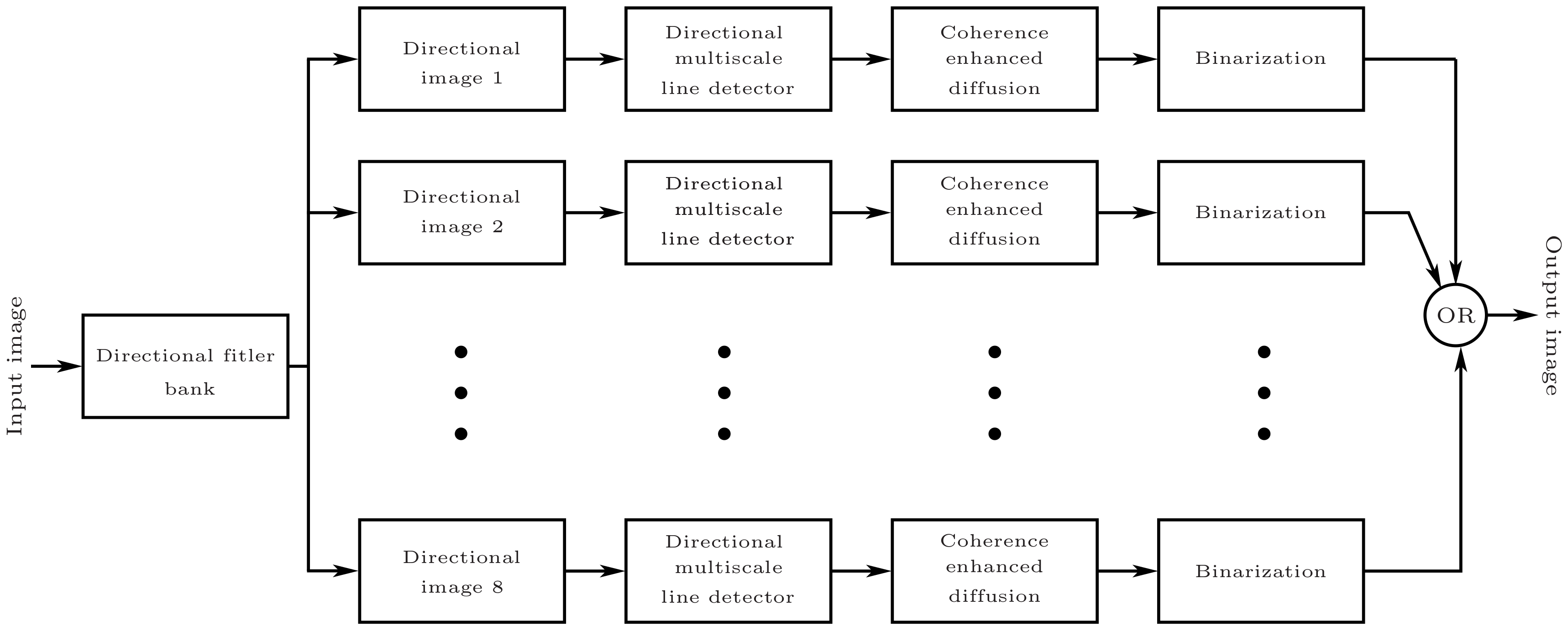
Figure 2 depicts the overall flowchart of the proposed technique. The major building blocks of the proposed methodology are outlined as follows:
Creation of direction-specific image array using bandpass Directional Filter Bank (DFB) on the green channel of a RGB retinal image.
Employing multi-scale line detection at the orientated image array.
Using the Coherence-Enhancing Diffusion (CED) technique to enhance the sharpness of the segmented directional vessels.
Individual binarization of these directional images followed by linear recombination to efficiently threshold the vascular structures.
3.1. Bandpass Directional Filtering for Direction-Specific Vessel Isolation
Orientation-selective linear filters can mirror the localized flow of the direction of lines in a sub-region of interest, such as ridge patterns and retinal vascular networks [
39]. Directional Filter Bank (DFB) is a similar kind of structure, which divides an image into corresponding set of orientation-field images. Each subsequent orientation-selective image relates to a discrete set of line segments with a narrow radial range. The frequency response of such an oriented bandpass filter can be further decomposed into its radial (
) and angular (
) components by the following equation:
Butterworth filter is selected to evolve
as:
where
denotes the bandwidth or the angular width.
depicts the center frequency, and
gave suitable results for the experiment.
was set up by a directional kernel suggested by Knutsson et al. [
40] as follows:
where
is the filter’s desired bandwidth. The span of desirable orientations is set in such a way that
, following which
, where
k represents the decomposed distinct directional images.
sets the filter’s orientation such that
. The scope of these directional filters is from 0 to
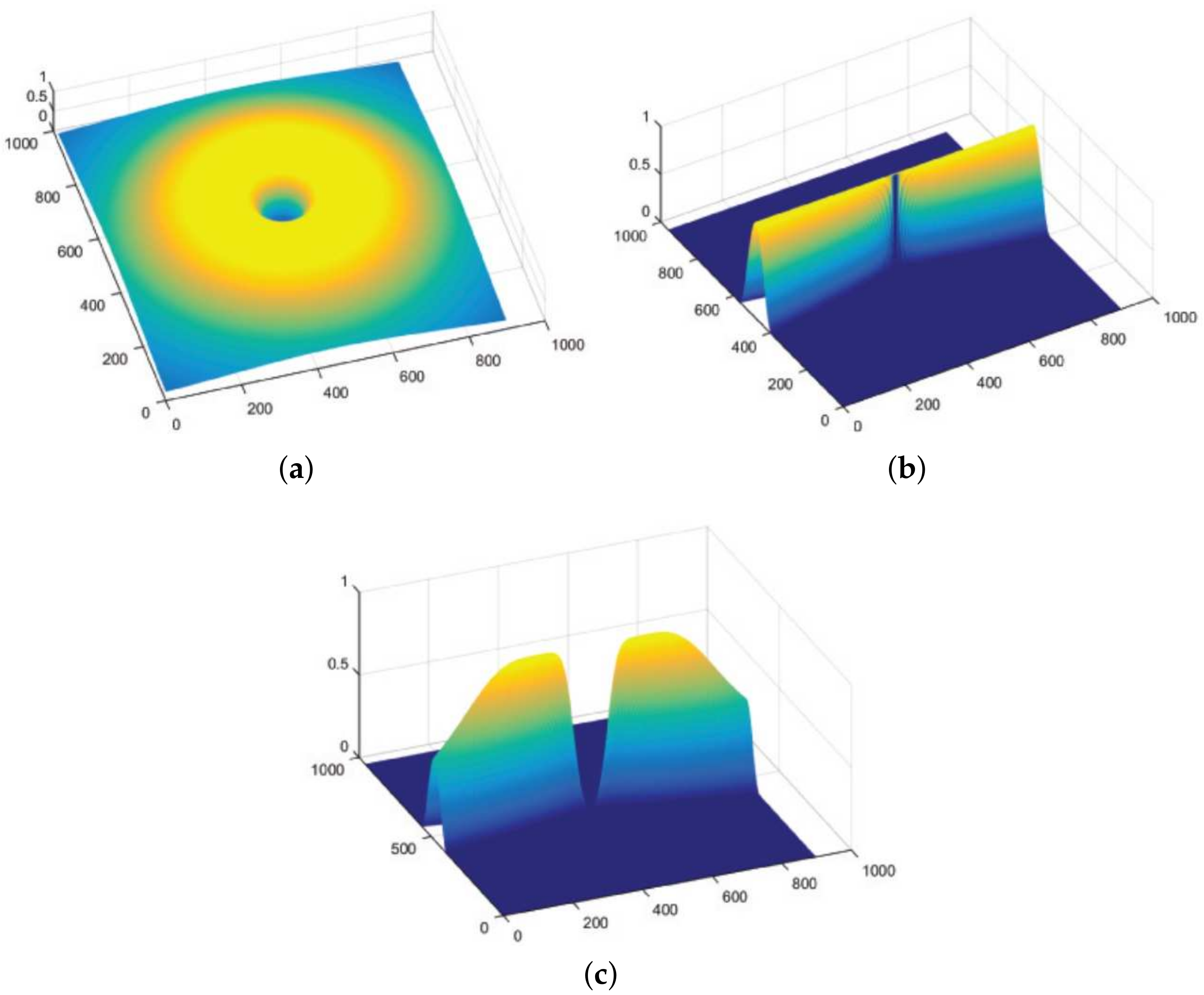
as they sum to unity. An example of a directional filter
is shown in
Figure 3. To deal with the retinal images, radial center frequency is set to a pixel width of 30, with a bandwidth of 60 pixels for vessel segmentation. In other words, a span of
is the preset angular width iteration with center frequencies placed in the middle of these bandwidths at
, and so on.
A retinal image
is fragmented into its constituent directional filter bank involving numerous images
, where
. Here
i denotes the iterative increase in angle of the directional images spanning from 0 to 180 degrees. For our experiment, these orientations are given by
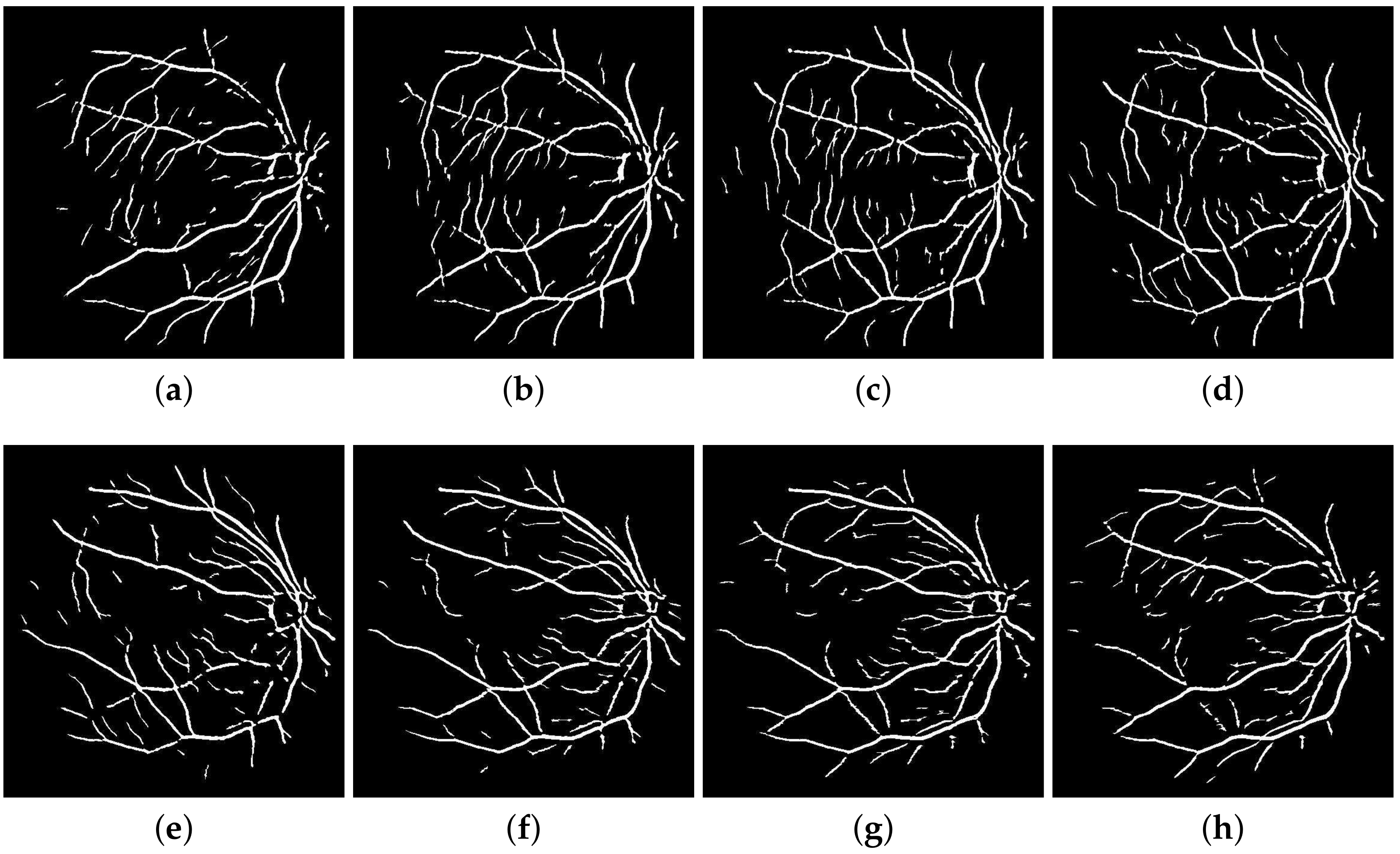
which cover the complete angular width at an interval of 22.5 degrees, thus constituting a total of 8 images. Following this regimen leads to the constituent directional images with a high vessel response in only the specified orientation and a dull response elsewhere. DFB technique thus helps decompose an input retinal image into a diverse set of directional images, thereby highlighting all vessels corresponding to their specific angles only. The directional filter bank similar to
Figure 3 was employed to help develop the direction-specific vessel images shown in
Figure 4.
3.2. Multi-Scale Line Detector
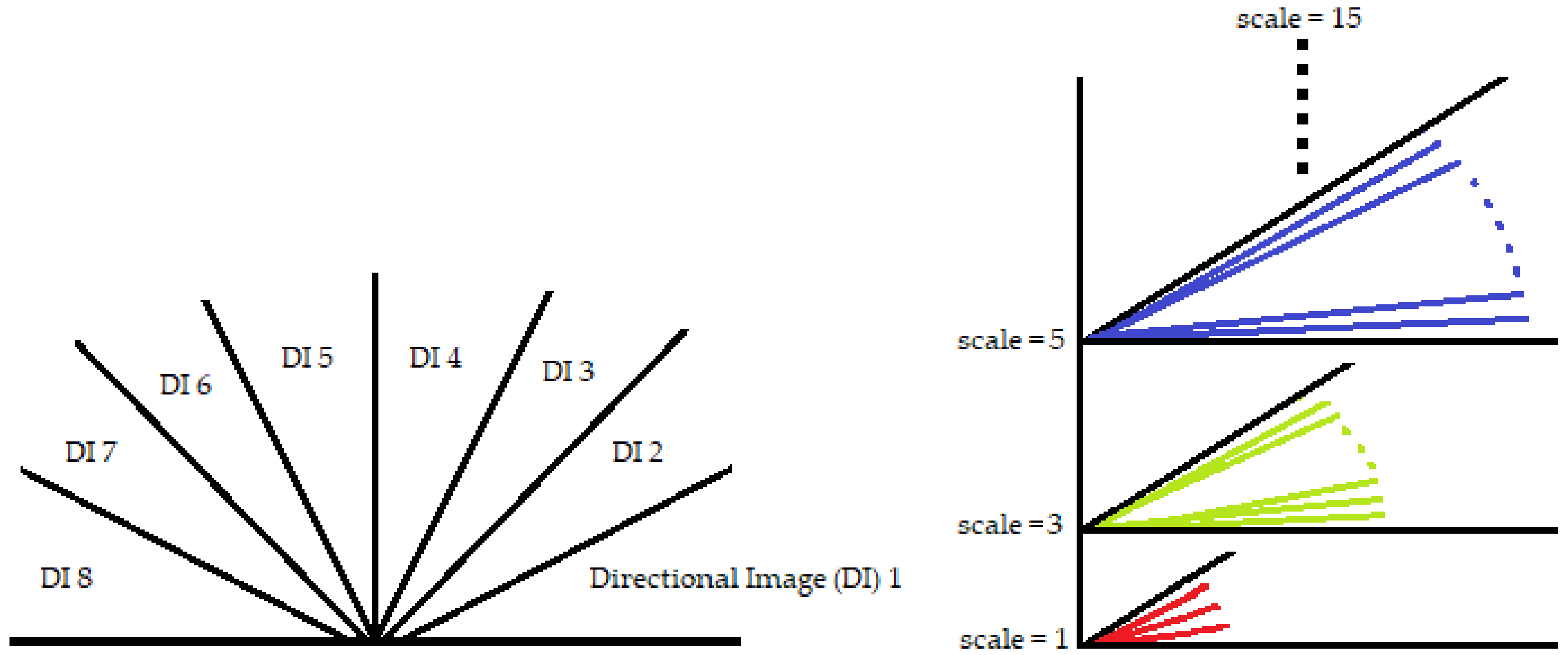
A rudimentary line detector works by matching the average grey-level response of a possible vascular segment with 12 scanning lines oriented at 15 degrees to each other. This 180-degrees scan investigates a sub-image of a particular window size (usually 15 pixels). The line with the highest intensity response is labeled as the ‘winning line’, which depicts the presence and orientation of a vessel whereas lower responses confirm their absence. Therefore, any arbitrary pixel is classified as either a vessel or non-vessel pixel depending upon its variance from the winning line.
Another critical issue where line detectors excelled over other techniques, is the problem of central light reflex. It occurs when the edges of vessels exhibit a heightened intensity as compared to their mid-lines. This reflex causes a lot of false positives as the pixels near the center of vessels get misclassified as background. Line detectors, on the other hand, remain largely unaffected due to the winning line methodology. However, there are some major drawbacks with the basic line detector, the most important of which is its tendency to combine close vessels. Also, vessel crossover points induce false vessel augmentations, and edges of major vessels cause misclassification of background pixels as foreground.
To mitigate these negative effects, Nguyen et al. [
26] suggested varying the scales of the scanning lines to distinguish vessel and background pixels, a technique he named as multi-scale line detectors. This was done by adjusting the length of the scan line
L from 1 to the window size
W, with the expectation that this would help alleviate the problems discussed above. Two intensity responses labeled as
(maximum line response), and
(average window response) were used to calculate the multi-scale line detector as:
This detector works brilliantly in all three problems faced by the basic line detector but reducing the detector’s line length introduces noise artifacts. This addition of noise comes from a narrower range of line detectors, leading to a weaker contrast among vessel and non-vessel pixels. To enhance the contrast, these raw response values are recombined in linear order to standardize these values to zero mean and unit standard deviation distribution as follows:
where
and
M are the standard and raw responses, respectively. The statistical values of
and
(mean and standard deviation of the raw values, respectively) help keep the distribution of intensity values in check. Therefore, these intensity values are extended over a broader range to significantly improve the contrast between the vessels and background, thereby reducing false positives.
Previously, the multi-scale line detectors were used to scan all the angles, and were not focused on any single direction. The method still worked remarkably well at detecting retinal vessels, but output response varied in contrast, making the detection process harder with a single threshold. This was due to the reason that, for an area having both types, the high contrast vessels dominated the detector’s focus and the weak contrast vessels got suppressed. Also, during the combined binarization process, tiny vessels, especially of 1-pixel width got wiped out. Not only the tiny vessels, but this difference in contrast also affected the major vessels as their borders were misclassified and thus narrowed down. Major vessels are often overlooked, but they are important as well when considering the overall efficiency of the segmentation process. For a major vessel having a width of 10 pixels, if the detector classifies 8 vessels correctly, that is still a loss of 2 pixels. Now looking at the percentage of major vessel pixels as compared to the tiny vessels in a retinal image, this loss of 2 pixels becomes a huge cumulative loss for the detector’s sensitivity.
Here lies the novelty claim in this method such that, multi-scale detectors are made to operate in a narrower directional range instead of the whole 180 degrees. Not only this, the images these detectors work on are also directional in nature as acquired from the DFB technique as shown in
Figure 5. This is done with the anticipation that, when both the image and filter’s directions are aligned, the filter’s response would be far superior, and features will be picked up more efficiently as depicted in
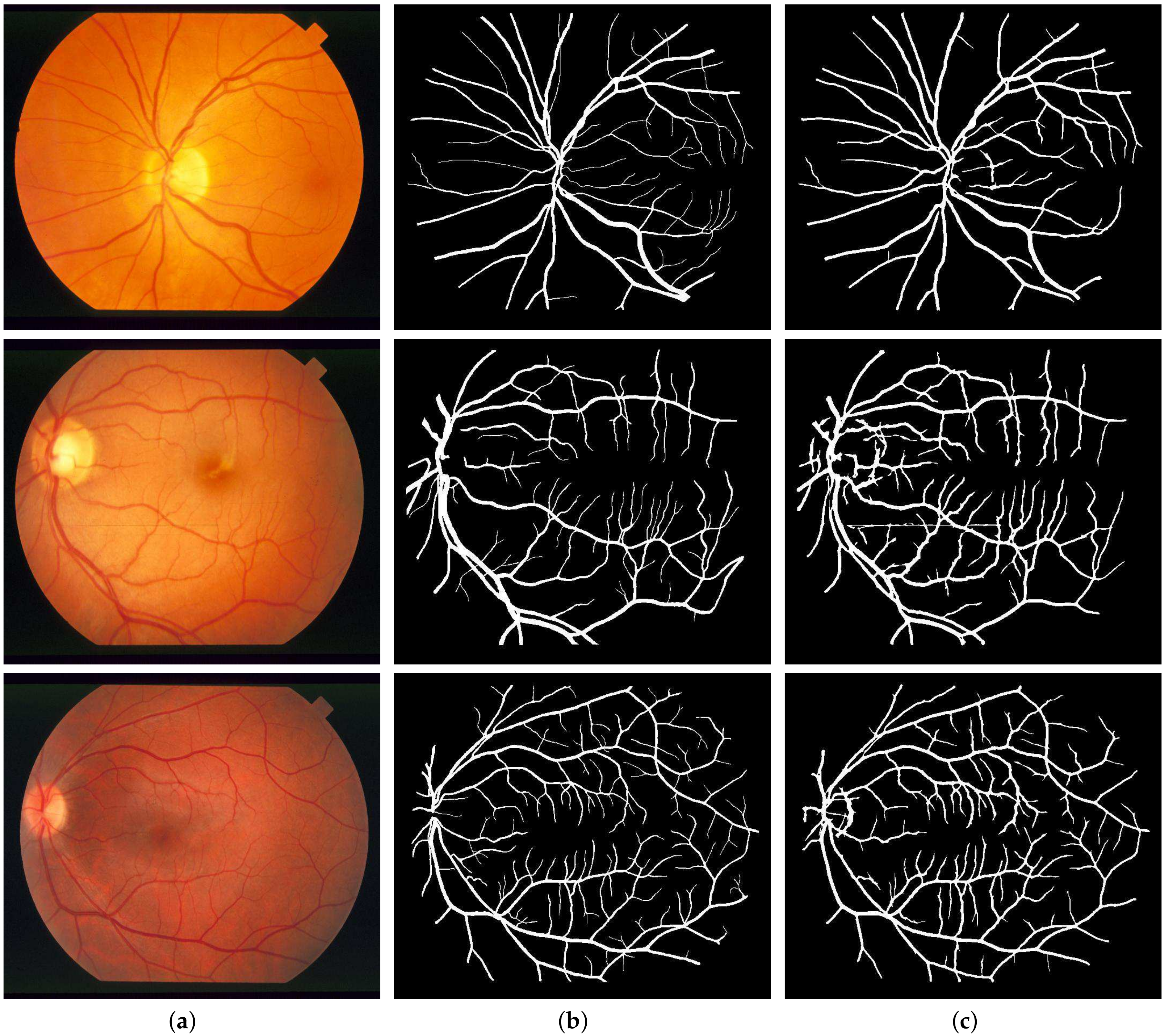
Figure 6. To top it all off, the binarization is also done within these distinct directions to achieve improved vascular segmentation as shown in
Figure 7.
The multi-scale line responses of every individual pixel are linearly recombined as:
Combined responses
of each of the 8 directional images are calculated separately where
d depicts the direction. These directional responses go through the binarization process before being accumulated into the final segmented image. The window size is taken as 15 in which each scale is averaged using the same weight. The parameter
represents the scale depth which is iterated from 1 till 15 with a step size of 2, thus resulting in a total of 8 scales.
represents individual scale responses calculated from Equation (
5), and
is the inverted green channel response of each pixel in the RGB image. The parameter
is included because the green channel information offers better contrast of the vessels as compared to other background entities such as OD and lesions [
26]. In an original green channel, the vessels are dark on a light background, whereas this paper makes use of inverted green channel where vessels are light on a dark background for better visibility. This linear recombination scheme results in the reduction of background noise in the proximity of vessels.
3.3. Coherence-Enhancing Diffusion (CED)
Regularization of variations in elongated structures is done by applying anisotropic diffusion through a diffusion matrix, also known as Coherence-Enhancing Diffusion (CED). This filter is nonlinear but isotropic in nature and is dictated by the diffusivity parameter which allows or denies the diffusion at every point of an input image. This diffusion is done based on the feature’s orientation at that point in such a manner so as to avoid smoothing across the edges and thus, preserve sharpness in the image. In other words, the diffusion or smoothing is to be guided parallel to the edges rather than over them. The efficiency of this process is monitored through the development of the Orientation Field (OF) on a point-to-point basis and thus, an accurate OF is crucial to the whole CED regimen. The diffusion matrix calculates the diffusivity parameters by observing the local image structure alongside the alignment towards clean directions at each diffusion step. Each valid change is noted in a secondary matrix known as a second-moment matrix (or structure tensor), which is an established method for enhancing flow-like structures. Assuming a retinal image
, the anisotropic scale-space for
is defined as:
where
D is the diffusion matrix of order
. This diffusion matrix is adjusted to the area under consideration by the symmetric structure tensor
, defined as:
where
,
and
represent the Gaussian derivative functions in both axes. The tuning parameter
is defined as:
Using this parameter, the two dominant eigenvalues become:
The expression comprehensively depicts the local variation of the gray values around a locality as follows:
; constant areas.
or ; straight edges.
; corners.
; flat regions.
The last pieces of the puzzle are the eigenvectors which are later integrated with the eigenvalues to reconstruct the diffusion matrix
D. One is the normalized eigenvector
, and the other is the orthogonal eigenvector
. The eigenvalues of the diffusion matrix are taken as:
where
, and
. The diffusion matrix
D can be recreated with its eigenvalues and eigenvectors as:
Overall, the diffusion process advances in the following four pivotal steps:
- 1.
Evaluate the second-moment matrix according to Equation (
8).
- 2.
Eigen-directions are computed using Equation (
10), and diffusion matrix is constructed using Equations (12), (13), and (14).
- 3.
Calculating change in intensity of each pixel based on its local neighborhood according to partial differential equation as .
- 4.
Update image using the diffusion equation:
3.4. Binarization
It is a thresholding technique that converts a gray-scale image to a binary image and therefore, is a crucial step in the effective segmentation and classification of foreground features. A threshold value dictates this binarization phase, where a value greater than a carefully calibrated threshold allocates that pixel position to foreground and other values are classified as background or vice versa. As discussed during the line-detector phase, different lengths of detectors produce different artifacts (shadows and extensions) within the image. Method in [
26] opted for multi-scale detectors as the detector had to move in all directions from 0 to 180 degrees. When a small length filter is aligned across a vessel, it produces shadows which cause false positives. This is not the case with our directional filter as the direction of the line filter is limited. However, the problem of extensions, which is caused by the larger scale filters still remains and is dealt with using traditional Niblack image thresholding [
41].
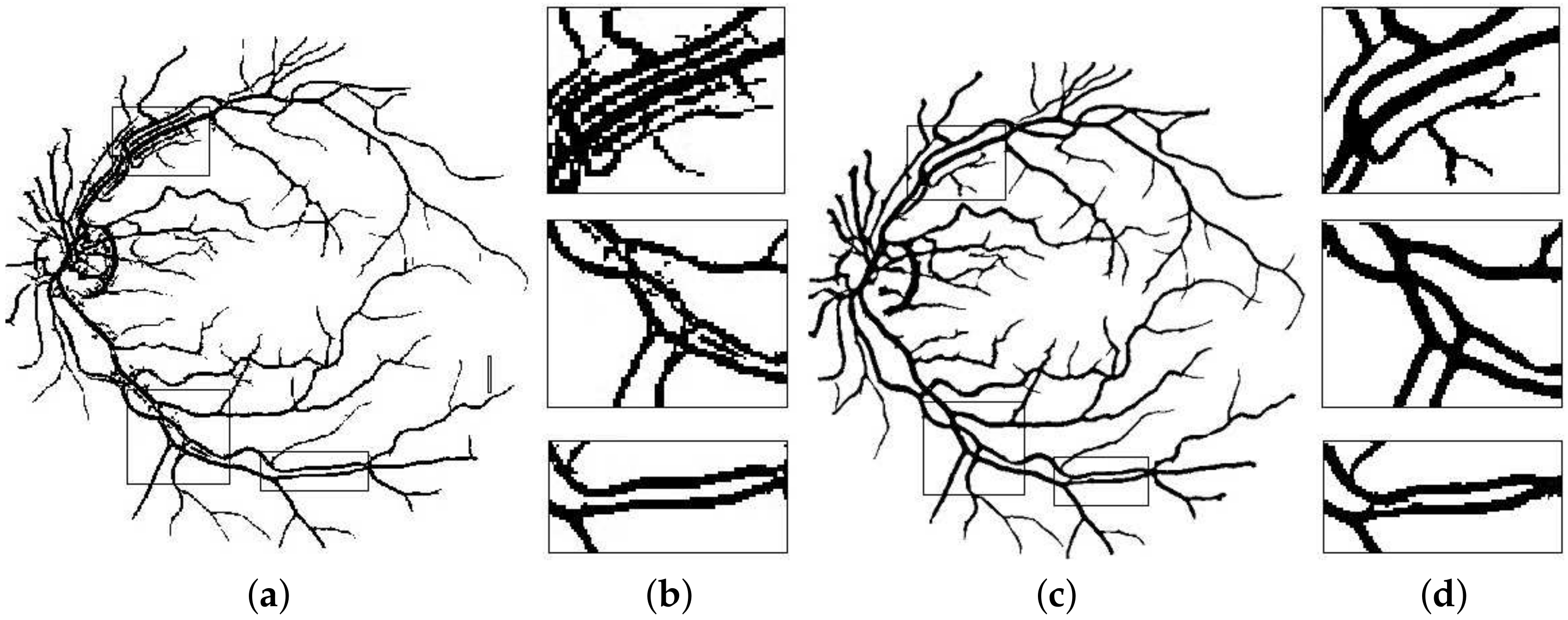
Extensions can be avoided by using a better binarization scheme that involves the line filter’s standard deviation. A 2-D fissure likelihood measure [
42], used to guide binarization process is defined as:
Here,
represents the line response of any arbitrary pixel while
and
depict the line filter’s mean and standard deviation at that point, respectively. The bias parameter
k is used to stabilize the impact of standard deviation from vessels of different sizes and Niblack proposed its value to be kept at −0.2. However, due to the sensitivity of the binarization process to this parameter, its values were tested from the range of −0.3 to 0.3, and the value of −1.5 was found to be suitable for this experiment.
Figure 8 depicts the effectiveness of this step towards mitigating the effects of extensions created by the line filter.
The extension removal process is followed by the Linde–Buzo–Gray (LBG) algorithm for scalar values [
43]. However, the initial cluster information is fed with Otsu method [
44] to avoid trapping in local minimum. The steps for LBG algorithm for our application are as follows:
Input pixel intensity values .
Initialize a codebook C= using Otsu method.
The initial codebook is split to create two values as and , where △ is a small positive number.
Classify the image pixels into two clusters according to if for .
Update cluster centers
,
by:
Set
and compute the distortion as:
If (a small positive number), repeat step 4 to step 6.
The final threshold value is:
