Abstract
Yield mapping is a subject of research in (precision) agriculture and one of the primary concerns for farmers as it forms the basis of their income and has implications for subsidies and taxes. The presented approach involves deployment of field harvesters equipped with sensors that provide more detailed and spatially localized values than merely a sum of yields for the whole plot. The measurements from such sensors need to be filtered and subject to further processing, including interpolation, to facilitate follow-up interpretation. This paper aims to identify the relative differences between interpolations from (1) (field) measured data, (2) measured data that were globally filtered, and (3) measured data that were globally and locally filtered. All the measured data were obtained at a fully operational farm and are considered to represent a natural experiment. The revealed spatial patterns and recommendations regarding global and local filtering methods are presented at the end of the paper. Time investments into filtering techniques are also taken into account.
1. Introduction
Precision agriculture is defined as “management strategy that gathers, processes and analyzes temporal, spatial and individual data and combines it with other information to support management decisions according to estimated variability for improved resource use efficiency, productivity, quality, profitability and sustainability of agricultural production” [1]. The main goals of (precision) agriculture are devoted to the maximization of economic profit on the one hand and the minimization of negative impacts on the environment on the other. The most tangible negative consequences of agricultural activities can be seen in the degradation of soil (e.g., erosion and the loss of organic content and/or biodiversity) and the pollution of (ground) waters by residues from fertilizers [2] as well as pesticides. In all such cases, precise spatial information is the key to the most efficient as well as sustainable usage of arable land
Conventional farming assumes that each field is a homogeneous area. For example, the same amount of fertilizer/pesticide is applied to each area of the plot. As stated by Aurenhammer [3], the concept of precision farming adds, among other things, the perspective of variable rate treatment. Precision farming techniques count and rely on the heterogeneity of a plot, defined in terms of so-called yield productivity zones (also known as management zones) that reveal areas with lower, average, and higher yields. The identification of yield productivity zones is the key to becoming more efficient from both the economic as well as ecological points of view. As such, the identification of yield productivity zones has been discussed for the last few decades (van Wart et al. [4], van Ittersum et al. [5] and Chen et al. [6]). Meanwhile, universal indirect methods are also being developed for the assessment of actual crop growth and yield on the basis of remote sensing (see e.g., Azzari [7], Bauer [8], Doraiswamy et al. [9], Lobell [10], Mirvakhabova et al. [11], Mulla [12] or Novoa et al. [13]).
Credible detailed data on crop yield can be used to determine variable rate treatments. Data from field harvesters represent the most detailed as well as the most credible source of yield information. In spite of this, field harvesters provide measurements with bias. Bias in datasets created by field harvesters corrupt the results, meaning that soil cannot be cultivated correctly. As suggested by Blackmore et al. [14] as well as Arslan et al. [15], such errors might arise for the following reasons: for example, the occurrence of unexpected events during the harvesting process, leading to unusual behavior on the part of the machine; the trajectory of the field harvester; errors caused by the wrong calibration of the yield monitor and presence of animals, adverse weather conditions, etc.
Measured yield data need to be filtered to reduce these biases, as documented by Gozdowski et al. [16], Spekken et al. [17], Sun et al. [18], Lyle et al. [19], or Leroux et al. [20]. These papers analyze the source of bias or errors during yield mapping [14,15,19] or propose various filtering methods or methodologies [16,17,18,20]. However, none of these papers attempts a comparison using statistical methods to identify the differences between various methods of yield data filtering.
Consequently, this paper focuses on a statistical analysis and filtering of data measured by field harvesters at the Rostěnice Farm in the Czech Republic (see Figure 1 and/or Figure S1, as well as Figure S2 in Supplementary for detailed information) between the years 2014 and 2018. Our research deals with filtering of farm machinery sensor measurements with regard to the yield of cereals. The research in this paper deals with certain types of field sensor data of cereals at a fully operational farm; more details are provided in Table 1.
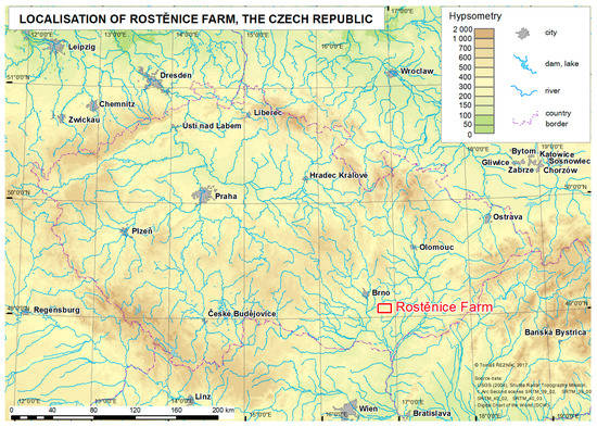
Figure 1.
Geographical location of the Rostěnice Farm.

Table 1.
Absolute number of sensor measurements, relative density of sensor measurements per hectare, and crops for each year and field.
The main goal of this paper is a relative comparison of interpolations from
- (Field) measured data;
- Measured data that were globally filtered; and
- Measured data that were globally and locally filtered.
So far, relative differences between the three interpolation approaches have not been analyzed in any previous research and remain open as scientific questions.
We seek answers to the following scientific questions (research objectives):
- What are the relative differences between interpolations from data measured by a field harvester and interpolations from identical data that are processed by global filters?
- What are the relative differences between interpolations from data measured by a field harvester and interpolations from identical data that are processed by global and local filters?
Our research, as presented in this paper, aims at statistical (spatial pattern) analyses of interpolations from data measured in a field on the one hand and filtered data (globally/globally and locally) on the other hand. Information on relative differences is required by both the agronomical practice as well as raised in the analyzed scientific papers as follow-up activities. The follow-up applied research is beyond the scope of this paper due to the extent and time constraints. Time investments into filtering techniques presented in the Discussion Section are the only exception.
2. Materials and Methods
2.1. Study Site
Data measured by a cereal field harvester were used to analyze and evaluate the approaches of spatial filtering and interpolation. Data acquisition was conducted at the Rostěnice cooperative farm in the south-eastern part of the Czech Republic (see also Figure 1). The farm, Rostěnice a.s. (N49.105 E16.882), manages over 8300 ha of arable land in the South Moravian region of the Czech Republic. The average annual rainfall is 544 mm and the average annual temperature is 8.8 °C. Within the managed land, the most prevalent soil types are Chernozem, Cambisol, haplic Luvisol, Fluvisol near to water bodies, and, occasionally, also Calcic Leptosols. The main programme is plant production, where the main focus is on the cultivation of malting barley (2500 ha), maize for grain and biogas production (2500 ha), winter wheat (2000 ha), oilseed rape (1000 ha), and other crops and products such as soybean and lamb. The average production intensity is 6 t/ha for malting barley, 7 t/ha for winter wheat, 10 t/ha for grain maize, and 4 t/ha for oilseed rape.
The fields are located in sloping terrain; for this reason, conservation practices with respect to soil tillage have been implemented to reduce soil water erosion. The farm has applied long-term soilless cultivation (mostly choppers) on its land, leaving all straw after harvest on the land. The high spatial variability of soil conditions in the southern part of the farm has led to the adoption of precision farming practices, such as the variable application of fertilizers (since 2006) and crop yield mapping by field harvesters (since 2010).
2.2. Sensor Measurements
Data were measured for two fields by a CASE IH AXIAL FLOW 9120 field harvester equipped with an AFS Pro 700 monitoring unit over three years: from 2014 to 2017 for the Pivovárka field and from 2016 to 2018 for the Přední prostřední field. Note that measurements for the Pivovárka field and year 2015 were not available due to failure of the monitoring unit. The measurements were of GNSS-RTK quality (Global Navigation System of Systems—the Real Time Kinematics), i.e., they provided a spatial resolution of less than 0.1 m (see e.g., Jedlička et al. [21]). Measurements were taken continuously each second at an average speed of 1.55 m·s–1, recommended as optimal at the Rostěnice Farm for cereal harvesting by the CASE IH AXIAL FLOW 9120 field harvester. The harvesting width was 9.15 m. The AFS Pro 700 monitoring unit was calibrated at 15 randomly selected locations to produce yield maps that were as precise as possible. Calibration of the AFS Pro 700 monitoring unit was based on explicitly measured weight of the field harvester’s container and harvested acreage. The used CASE IH AXIAL FLOW 9120 field harvester could not measure the weight by itself, weight measurements were therefore external. Such calibration was an iterative process, repeated three times as a standardized action of the Rostěnice farm. The monitoring of yield was conducted as on-the-go mapping by recording grain flow and moisture continuously over the whole plot area. The spatial distribution of the measured yield values at Rostěnice Farm is shown in Table 1. The crop type did not influence the spatial density of the performed measurements.
The measurements were stored directly in the field harvester and manually copied to a USB flash drive after the end of operations on the pilot fields. The conceptual schema for measurements by a field harvester follows ISO 19156 Geographic information—Observations and Measurements [22]. The results of measurements comprise the locations and attributes described in the UML (Unified Modelling Language) class diagram in Figure 2. The used data model represents a specialization of the Open data model for precision agriculture, as defined by Řezník et al. [23]. Figure 2 depicts the ISO 19156 schema only partially; the class “TrackingResult” demonstrates the specialization of the ISO 19156 generic abstract class “Result”.
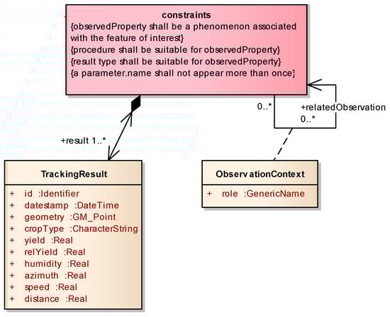
Figure 2.
The UML (Unified Modelling Language) class diagram of the data model used for measurements. The data model represents a conceptual specialization of ISO 19156 (not depicted fully due to its complexity; focusing only on the specialised class “TrackingResult”).
2.3. Filtering of Yield Data
Our approach regarding the filtering of measured data can be divided into two parts—the cleaning of global and local outliers as follows:
- (a)
- The cleaning of global outliers (hereinafter global filtering) removes non-credible values within the whole dataset by means of the statistical analysis of attribute values, namely yield measurement, speed of the vehicle, or direction of vehicle movement (see also the UML sequence diagram in Figure 3).
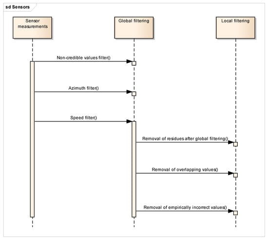 Figure 3. The overview UML sequential diagram of global and local filtration methods.
 - (b)
- The cleaning of local outliers (hereinafter local filtering) focuses afterwards on particular parts of the dataset in a higher level of detail, and is mostly based on the neighborhood of data point values or pattern recognition.
Details of both global and local filtering are described in greater detail below, as well as in the results section. A general processing sequence is depicted in Figure 3.
Global filtering uses statistical, i.e., non-spatial, analyses and methods for detecting non-credible (yield) values. Non-credible in this sense means that there is a high probability that (1) a value in a given location was measured incorrectly, or (2) a value was not achievable within the measurement process, or (3) the conditions of measurement do not seem credible.
Three global filters were used for detecting incorrect outliers:
- the range of realistic yield values;
- the direction of harvesting;
- the speed of a field harvester.
The range of realistic yield values follows the thresholds established by the structure of the data, both empirically and on the basis of the frequency curve (see Equation (1)).
where:
- vs: harvester velocity,
- μ: mean velocity,
- σ: standard deviation of velocity.
The statistical file follows normal distribution. The measured data were considered as significant within the interval of two times the standard deviation, i.e., 95.5% of all values. Such a value was also discussed with, and approved by, the agronomists at the Rostěnice Farm. In other words, points outside the threshold values of 50%, and 150% for relative yield were considered nonrealistic and were excluded from the dataset (the average value of the relative yield for the whole dataset was 100%). Such interval also corresponds to ± 2 standard deviations. We accepted the removal of some realistic values as a lower threat in comparison to keep keeping non-realistic values in a dataset intended for interpolation; this view is based on the assumption of agronomists from the Rostěnice farm as well as exploratory statistical analyses of measured fields.
The second global filter selected the points that were harvested in a direction different to the dominant direction(s). Such selection applies mainly to peripheral areas of fields, so-called headlands, that are from a trajectory point of view cultivated in a different way to the rest of the field.
The third global filter was based on the speed of a field harvester. The speed of a field harvester should be as constant as possible to ensure data are valid. The amount of measured yield is different if a field harvester passes with a considerably lower or higher speed. A harvesting speed of 1.55 m·s−1 was the mean value for speed measurements (as also indicated in Section 2.2). Harvesting speed influences yield measurements. The lag time between harvesting in a certain position and sensor measurement was equal to 12 s. The locations of measurements can be degraded in cases where a field harvester is considerably faster or slower than the mean speed. Values excluded by the global speed limitation filter were those that exceeded the limit of three times the standard deviation, i.e., 0.3% of the measured values.
Local filtering focuses on data in greater detail and is based on differences between neighboring cells and/or patterns. A decision on the credibility of analyzed data needed to be made also in this case. General algorithms with various flexibilities have been developed for local filtering [18,19]. Such universality comes at a price, however, as none of the developed algorithms can provide sufficient results in all analyzed cases, i.e., for all years and for all fields. Basically, the more general the algorithm is, the wider its usage, but the results are less precise. Local filtering brings the most precise results with regard to domain knowledge, e.g., measurements, the processing of data, and the history of the yield, the knowledge of the data, of the situation, and of the problematics in general. The development of other general local filtering algorithms was beyond the scope of this paper due to the time and effort such a task would require. Local filtering comprises a set of subjective methods. In general, points are excluded manually.
2.4. Applied Interpolation Methods
Interpolation methods were used to compare, verify, and evaluate the differences between interpolated surfaces derived from field sensor measurements that were (1) obtained directly from the field harvester, (2) processed by global filters, and (3) processed by global and local filters. The preconditions for the Simple Kriging method were met [24,25]. When following Cressie [24], it is assumed that we know µ exactly, and also that data locations are known. It was confirmed that the data of measured values had normal distributions, were homogeneous, and did not show any significant trends. The parameters of the interpolations of each model were computed by means of Exploratory Spatial Data Analysis (also known as ESDA) in ArcGIS 10.6 software.
2.5. Verification Methods
Map algebra was used for the spatial comparison of measurements that were (1) unfiltered, (2) filtered globally, and (3) filtered globally as well as locally. The relative differences were used as defined in Equation (2). Relative differences are often used as a quantitative indicator of quality assurance and quality control for repeated measurements where the outcomes are expected to be the same.
where:
- dv: relative value difference (%),
- va: unfiltered interpolated yield value,
- vb: filtered interpolated yield value.
Statistical comparison required several transformations. First, interpolated raster data (the comparison of data measured by a field harvester, data that were processed by global filters, and data that were processed by global and local filters) needed to be converted to discrete points. These points were distributed regularly, and their distances corresponded to the pixel sizes of the input raster (5 m). In addition, the attribute values of these points were statistically analyzed. Due to the frequency of points and the size of the studied fields, it was expected that attribute values would have a normal distribution. Student’s t-test [26], specifically the dependent two-sample t-test, was chosen as the appropriate statistical test.
3. Results
3.1. Global Filtering
Thresholds for the range of yield values were defined as described by Equation (1). Figure 4 depicts the distribution of values as a histogram. It is assumed that values lower than 50% and higher than 150% of relative yield were the result of errors that occurred during the measurement process. Another source of this kind of error might be unexpected events or conditions on the field—for example, missing crops on part of the field (because of animals, weather, etc.). Examples of excluded points as well as comparisons between years can be seen in Figure 5.
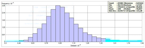
Figure 4.
Distribution of measured yield values at Přední prostřední field in 2017 (excluded values highlighted by light blue color).
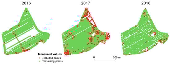
Figure 5.
Excluded points with non-credible values of very high and very low relative yield in the field Přední prostřední. The identical global filter was used.
The second global filter aims at the direction of harvesting as described in Section 2.3. In general, farmers do not consider headland areas as (1) yield prosperous areas or as (2) representative sensor measurement areas. There are mostly ecological reasons for the different harvesting directions applied to headland areas. The global filter on direction also excluded the turns the field harvester had to make between areas. Considering directions different to the dominant direction(s) within the main area of the field, these data did not seem credible either. Two major errors were observed. Firstly, when the field harvester was not moving in a straight line, the cutting bar did not collect the crop regularly because the angle of ‘attack’ was changing. Secondly, data from locations that were harvested in a direction different to the dominant direction were non-credible. According to Figure 6, it seems that the Přední prostřední field was divided by a temporary road in 2018 (this was confirmed by the agronomists at the Rostěnice Farm).
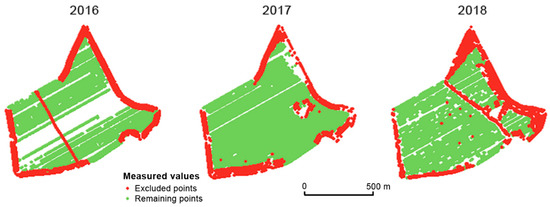
Figure 6.
Points excluded by the dominant direction global filter in the Přední prostřední field.
The prevailing direction of harvesting needed to be set specifically for each field, and it was defined through an azimuth. In some cases, however, the field harvester did not follow straight lines but curves. We identified several influencing factors, of which the terrain was the most important. The prevailing azimuth values for both fields were set from 50° to 70° in one direction and from 230° to 250° in the reverse direction (see Equation (3) and Figure 6). Measurements beyond the azimuth thresholds were removed.
where:
- α: azimuth of harvester trajectory,
- ,: ranges of valid azimuth values.
The third global filter aims at the speed of a field harvester. Areas in which the speed of the field harvester was very low correlated with higher measured values of yield and vice versa. According to agronomists at the Rostěnice farm, the speed of the field harvester changed for the following reasons: obstacles in the field, mechanical issues with the field harvester, or the behavior or inattention of the driver. Areas excluded by the global speed limitation filter are depicted in Figure 7.
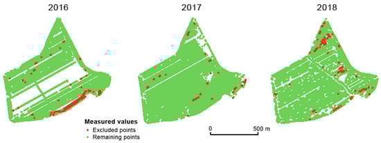
Figure 7.
Points excluded by the global speed limitation filter in the Přední prostřední field.
Figure 8 shows the measurements excluded by three global filters. Two conclusions may be reached. Firstly, the excluded measurements appear mainly in headland areas. Secondly, the excluded measurements vary considerably over the years (see Figure 8). It is assumed that the points excluded by means of global filtering are errors made during the harvesting process as well as during the measurements themselves. Any spatial correlation between excluded measurements across years was not proven.
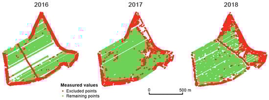
Figure 8.
Points excluded after applying all three global filters (extremely low/high relative yield, dominant direction, and speed limitation) in the Přední prostřední field.
3.2. Local Filtering
Several issues were considered with respect to local filtering. First, overlapping measurements from the positional point of view were removed. In such cases, identical areas were “harvested” and therefore logged twice in the measured data. Values close to zero were measured during the second pass as almost the whole yield was harvested in the first pass. An example of an overlapping trajectory is depicted in Figure 9a. Local filtering methods analyze those areas again and remove leftover erroneous measurements.
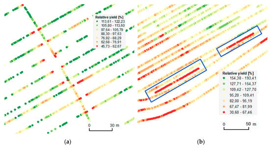
Figure 9.
Examples of overlapping (a) and partially overlapping (b) trajectories. The single-oriented trajectory was the first, while all the remaining trajectories depict the subsequent movements of the field harvester. Measured data were divided into classes according to the Jenks Natural Breaks method [25].
Figure 9a represents the most obvious case of overlapping trajectories. In many other cases, trajectories were not crossed explicitly. That is, trajectories were overlapped only by a portion of the cutting bar, as depicted in Figure 9b. In such cases, the partial use of the cutting bar leads to non-representative values.
The cutting bar of the field harvester in the conducted pilots was 9.15 m wide. The values of any points in neighboring rows lying within the adjacent path of the cutting bar are misleading and can therefore be considered as errors. As confirmed by the Rostěnice agronomists, overlaps of this kind usually occur because crop leftovers must be harvested.
The third applied local filter targeted the gaps in measurements within rows; see also Figure 10. In many observed cases, gaps within rows were connected with a decrease in the measured yield. Sudden decreases occurred for example when the field harvester had to raise its cutting bar in order to avoid an obstacle.
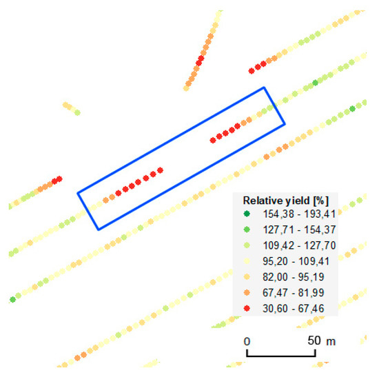
Figure 10.
Example of gaps in measurements within a row.
Erroneous measurements with sudden decreases in values were also observed at the ends and beginnings of gaps in measurements within a row. Such patterns were observed when a part of the crop was missing because of weather (strong rain and hail, drought, etc.), animals, or other unexpected events. The causes of such gaps—and therefore the respective decreases in measured yield—were often unique to the particular harvest or year, as no correlation was identified across years. The majority of such erroneous measurements were excluded by global filtering. Values of neighboring rows were also taken into account to distinguish between errors and coincidences when gaps correlated with zones with lower yield.
Figure 11 together with Table 2 and Table 3 depict the spatial distribution as well as the absolute amounts of measured data that were filtered by means of global as well as local filters. A considerable number of measurements were excluded in the case of the Přední prostřední field in 2018 because of headland areas and because of the high number of gaps inside the field. The year 2018 was extremely dry in this part of the Czech Republic, which had an impact on the yield and on the number of gaps.
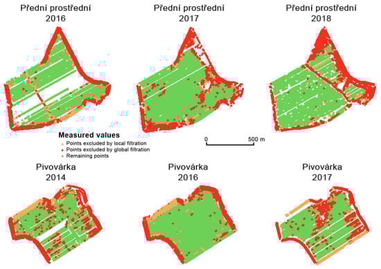
Figure 11.
Spatial distribution of measurements filtered by means of global and local filters.
Table 2.
Absolute values of measurements filtered by means of global and local filtering for the Přední prostřední field.
Table 3.
Absolute values of measurements filtered by means of global and local filtering for the Pivovárka field.
3.3. Interpolation of Yield Data
Interpolations were made for all datasets (see Figure 12 and Figure 13). Simple Kriging was used as an interpolation method, as mentioned in Section 2.4; the parameters are presented in Table 4 and Table 5. For filtered data, spatial extents were smaller due to global filtration. In order to achieve homogeneous (consistent) and comparable results, we decided not to use extrapolation methods, as their precision in the respective areas would have been debatable.
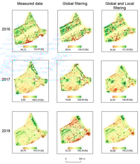
Figure 12.
Interpolations of measured, globally filtered, and both globally and locally filtered data for the Přední prostřední field (%).
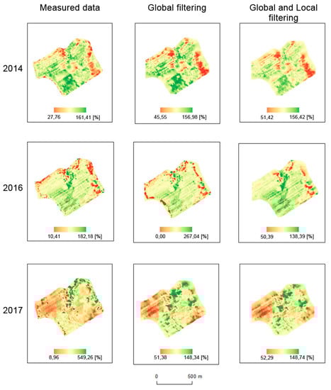
Figure 13.
Interpolations of measured, globally filtered, and both globally and locally filtered data for the Pivovárka field (%).
Table 4.
Exploratory Spatial Data Analysis (ESDA) results for setting up the Simple Kriging interpolation for the Přední prostřední field. Parameters were computed separately for (1) interpolation from measured data, (2) interpolation from measured data that were processed by global filters, and (3) interpolation from measured data that were processed by global and local filters.
Table 5.
ESDA results for setting up the Simple Kriging interpolation for the Pivovárka field. Parameters were computed separately for (1) interpolation from measured data, (2) interpolation from measured data that were processed by global filters, and (3) interpolation from measured data that were processed by global and local filters.
3.4. Verification of Sensor Measurements versus Filtered Data
The statistical analyses provided answers to the question of differences between interpolated surfaces. There were significant differences between the
- measured non-filtered data and measured data filtered by means of global filtering in six cases at a significance level of 95%;
- measured non-filtered data and measured data filtered by means of global and local filtering at a significance level of 95% in all cases.
The results of statistical analyses are depicted in Table 6. Means, medians, standard deviations, testing criteria (t-score), and values (p) are provided for both fields and all years. Spatial relative differences, as depicted in Figure 14 and Figure 15, reveal the following spatial patterns:
Table 6.
Descriptive statistics and results of dependent t-test for paired samples. As the number of comparison points was large and the mean and median values were different by less than 10% in all cases, we expect a normal distribution.
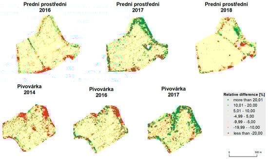
Figure 14.
Relative difference between unfiltered data and data filtered by global filtering.
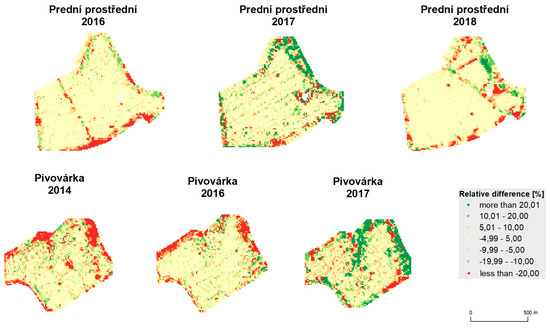
Figure 15.
Relative difference between unfiltered data and data filtered by global and local filtering.
- mean values appear inside the fields;
- deviations appear at the edges of the fields and around green infrastructure (groves);
- less commonly, deviations also appear inside the fields, mostly because of trajectory overlaps;
- influences of terrain and water flow accumulation characteristics appear in extreme climatic conditions (see Pivovárka field in 2017 as the most visible example).
Table 7 and Table 8 quantify the spatial distribution statistically. They depict the percentage of the area of the whole field that belongs to a relative difference category.
Table 7.
Relative difference between measured data and globally filtered data, and measured data and both globally and locally filtered data for the Přední prostřední field (%).
Table 8.
Relative difference between measured data and globally filtered data, and measured data and both globally and locally filtered data for field Pivovárka (%).
4. Discussion
The basic scientific questions raised at the beginning of the paper deal with the benefits of both global and local filters. We may formulate the following discussion points based on the achieved results. The presented discussion points are structured with the following logic. Point (a) compares the achieved results with results from related papers. Points (b) and (c) target usability issues of global and local filtering. Points (d), (e), and (f) summarize lessons learned from applications and verifications of filtering techniques.
- The differences between (1) measured data, (2) measured data filtered globally, and (3) measured data filtered globally and locally were discovered as considerable in the analyzed fields and years. Similar results were achieved by Spekken, Anselmi, and Molin [17]. By comparing the global method (based on the removal of outliers from the histogram) and the local method proposed by Spekken, Anselmi, and Molin [17], it was similarly confirmed that local filtering has the effect of a low-pass filter as in other kinds of image processing domains (see e.g., Zhou et al. [27] for low-pass filtering).
- Global filtering represents a set of universal approaches that may be applied to any field. It was confirmed that global filtering is a must to eliminate high-level bias. The statement by Vega et al. [28] was also confirmed in our study, i.e., that global filtering improves yield distributions, while local filtering impacts the yield spatial structure for output interpolations and yield maps.
- The benefits of local filters were as follows:
- ○
- The shape of a field: a convex shape lowers the need for local filtering. The more the shape of a field differs from a convex one, the higher the probability of crossed trajectories is, these causing bias in interpolations as well as in interpretations.
- ○
- The variability of a relief: in particular, narrow valleys with steep slopes in a field require higher filtering efforts. Such areas, as depicted for instance in Figure 16, were characterized as areas with considerably higher yields than the average for the field. The conducted measurements showed that yields in such narrow valleys within a field may reach 150% of the average for the whole field or even higher. Agronomists at the Rostěnice Farm also confirmed that such very productive strips of land had existed there for the last two decades. It was stated that underground water from the slopes moves to the bedrock of the valley and, together with transported nutrients, creates a supernormal strip of fertile land. In such cases, a field harvester moves first along the bottom of the narrow valley and subsequently follows its “normal” trajectory, as planned for the whole field; see also Figure 16.
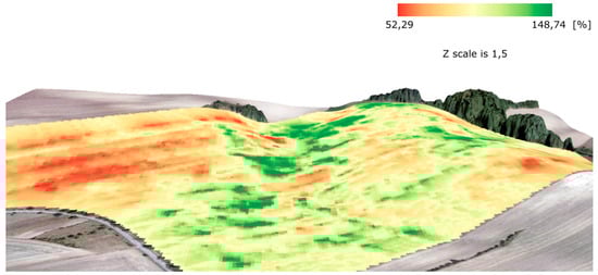 Figure 16. 3D visualization of the measurements processed by means of global and local filtering for the Pivovárka field in 2017. Note the valley with a yield close to 150% of the average for the whole field (in green).
- Harvesting strategy: in general, the measurement functions differ when a field harvester goes from an area that is being harvested into an area that has already been harvested and/or is not intended for harvesting and vice versa; see Figure 17. When a field harvester goes from an area that is being harvested into an area that has already been harvested and/or is not intended for harvesting, the measured values fall to zero almost immediately. In contrast, when a field harvester goes from an area that has already been harvested and/or is not intended for harvesting into an area that is being harvested, the measurements are not continuous in the analyzed fields for an interval of between 5 and 30 m. In our study, this interval varied considerably while no universal influencing factor was revealed. As depicted in Figure 12 and Figure 13, the interpolation from measured data creates so called bull’s eyes (as also described by Wilson et al. [29]; Garnero et al. [30]). Such a phenomenon results in the prediction of very low values, i.e., close to zero, in the interpolated positions. In contrast, global as well as local filters have a smoothing function. A simple rule may be defined that local filters have a higher smoothing function than global filters, as clearly visible in Figure 17.
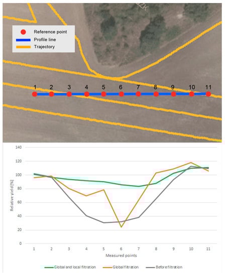 Figure 17. The differences in relative yield values for (1) interpolation from measured data, (2) interpolation from measured data that were processed by global filters, and (3) interpolation from measured data that were processed by global and local filters.
 - This paper brought answers from the statistical point of view concerning differences among interpolations from filtered and non-filtered data. Applied sciences deal in this case, among others, with time and/or financial investments into different kinds of filtering. Three fields in Rostěnice farm, different from those used for statistical evaluations, were used to compute the time investments into various techniques presented in this paper. The results of time investments are presented in Table 9, broken down according to interpolations from (1) measured data that were globally filtered, (2) measured data that were locally filtered, and (3) measured data that were globally and locally filtered. Results presented in Table 9 can be summarized as follows:
Table 9. Time investments for interpolations from (1) measured data that were globally filtered, (2) measured data that were locally filtered, and (3) measured data that were globally and locally filtered.
- ○
- Global filtering is a simple task, i.e., it required on average about three times less time than local filtering. The process of global filtering could potentially be more automatized than in this study, which would decrease the time investments even further.
- ○
- Time investments into local filtering vary considerably among the fields. The number of measured points and the area of a field are the main drivers for time investments. Local filtering techniques also require local knowledge from the farm in order to apply a local filter accordingly. Time investments into local filtering shown in Table 9 are valid only for the cases in which a person performing the filtering and interpolations has local agronomical knowledge in the analyzed field. However, this was not our case, and therefore we needed two more hours on average for a field to discuss the filtering parameters with agronomists at the Rostěnice farm. In our case, the additional 2 h on average for a field were required to search for notes from the field, verify related evidence in the Farm Management Information System (FMIS), etc. It was confirmed that no general guidance for local filtering can be given.
- ○
- Table 9 also depicts a “time index” that expresses the relative time investments in minutes per hectare.
- We may identify two main subjects for discussion from the spatial accuracy point of view:
- ○
- In theory, the maximum positional error for the conducted measurements could be up to 18.6 m, though, in practice, such a value would be improbable. The positional error is influenced by two factors. The first is the speed of the harvester—in our study, this was 1.55 m·s−1, which was recommended as optimal at the Rostěnice Farm for cereal harvesting with a CASE IH AXIAL FLOW 9120 field harvester equipped with an AFS Pro 700 monitoring unit. The second is the delay between the collection of grain and the computation of the respective yield—in our study, a period of 12 s. The CASE IH AXIAL FLOW 9120 field harvester equipped with an AFS Pro 700 monitoring unit automatically links the computed yield value to the corresponding position, i.e., the position in which the field harvester was 12 s before. A positional error may arise when the speed of the field harvester is considerably higher or lower than the recommended one, meaning that the yield is not computed correctly for the corresponding position.
- ○
- The positional error caused by the GNSS-RTK receiver was in centimeters. This means that the bias in measured positions resulting from the GNSS-RTK measurements could be considered negligible when considering the changing speed of the field harvester.
5. Conclusions
The presented paper in a novel way statistically and spatially evaluates the extent between non-filtered and filtered data measured by field harvesters. Similarly, from the originality point of view, time investments into filtering techniques were expressed as well. Among others, “time index” that expresses the relative time investments was provided as well for transferability and comparability of results.
The conducted yield measurements and subsequent data processing were performed to test the scientific questions raised at the beginning of the paper:
- At a confidence level of 95%, there is a significant difference between interpolations from data measured by a field harvester and interpolations from the identical measured data processed by global filters.
- At a confidence level of 95%, there is a significant difference between interpolations from data measured by a field harvester and interpolations from the identical measured data processed by global and local filters.
Both scientific questions were answered with respect to measurements of cereals in two fully operational Czech fields. The measured data may be influenced by a bias due to calibration. This paper addressed such a bottleneck by means of the relative comparison of measured data, and global and local filtering instead of using absolute measured values. The bias in the measured data did not have a considerable influence on the comparison of the resulting rasters.
It was confirmed that global filters are a must for any interpolations and/or interpretations. Local filters, on the other hand, lose their importance when all of the following conditions are met:
- the shape of the analyzed field is convex;
- the analyzed field is flat from a vertical perspective;
- the recommended speed of harvesting is constant and follows the recommendations for the performing field harvester;
- there are no barriers within a field, such as
- green infrastructure like forest islands or wetlands,
- technical infrastructure comprising poles for electrical cables, water infrastructure for ameliorations etc.,
- geodetical and other signs,
- other kinds of barriers such as stones, because of which the harvesting height above the ground needs to be adjusted;
- crops, in our case cereals, are not damaged due to hailstorm and/or any other similar phenomena;
- trajectories of a field harvester are not crossed.
Local filters become valuable when any combination of the above-mentioned conditions are not met. In general, local filters are, from a spatial perspective, often used for headlands and buffers around barriers. The topic of local filtering goes beyond the scope of this paper due to its complexity as well as need of detailed local knowledge from farm agronomists.
The presented six conditions are also important for algorithms that aim to set the optimal trajectory of farm machinery. As far as the authors know, no algorithm has been developed that would take into account the complexity of all six conditions. The further development of track-optimizing algorithms is needed because of the use of autonomous and, more commonly, semi-autonomous farm machinery under the Controlled Traffic Farming approach. Semi-autonomous driving has become a common feature of farm machinery as it automatically enables such machinery to follow defined trajectories in lines, with human-driver input required only for the negotiation of headlands and/or barriers.
The conducted research is also a resource for further research that will attempt to compare the measured yield with that predicted from yield productivity zones. In the cases of both measurement and prediction, such yield productivity zones are interpolated surfaces. The resulting interpolated surfaces are significantly influenced by the applied filtering techniques. Filtering therefore influences the evaluation of yield productivity predictions that are confronted with measured values.
Supplementary Materials
The following are available online at https://www.mdpi.com/1424-8220/19/22/4879/s1, Figure S1: Fields managed by Rostěnice farm and hypsometry; Figure S2: Fields managed by Rostěnice farm and actual land cover.
Author Contributions
Conceptualization, T.Ř.; Data curation, T.P., V.L. and P.S.; Formal analysis, Š.L.; Funding acquisition, T.Ř.; Methodology, T.Ř.; Supervision, T.Ř.; Validation, L.H.; Visualization, T.P. and L.H.; Writing–original draft, T.Ř., T.P. and L.H.; Writing–review & editing, T.Ř., Š.L., V.L. and P.S.
Funding
This paper is part of a project that has received funding from the European Union’s Horizon 2020 research and innovation programme under grant agreement No 818346 called “Sino-EU Soil Observatory for intelligent Land Use Management” (SIEUSOIL). Tomáš Pavelka and Šimon Leitgeb were also supported by funding from Masaryk University under grant agreement No. MUNI/A/1576/2018 titled “Complex research of the geographical environment of the planet Earth”.
Acknowledgments
The authors would like to thank all persons from the Rostěnice Farm who participated in the study, from the drivers of farm machinery to the farm’s agronomists.
Conflicts of Interest
The authors declare no conflict of interest.
References
- Zimmerman, C. ISPA Definition for Precision Agriculture. 2019. Available online: http://agwired.com/2019/07/11/ispa-definition-for-precision-agriculture (accessed on 12 August 2019).
- Lipiński, A.J.; Koronczok, J.; Oblicki, M.; Choszcz, D.J.; Konopka, S.; Kolankowska, E.; Jadwisieńczak, K.; Majkowska-Gadomska, J. Analysis of changes in nutrient content in a soil in the context of possibility of variable application of mineral fertilizers use. Przemysł Chem. 2018, 97, 741–745. [Google Scholar] [CrossRef]
- Auernhammer, H. Precision farming-the environmental challenge. Comput. Electron. Agric. 2001, 30, 31–43. [Google Scholar] [CrossRef]
- Van Wart, J.; Kersebaum, K.C.; Peng, S.; Milner, M.; Cassman, K.G. Estimating crop yield productivity zones at regional to national scales. Field Crops Res. 2013, 143, 34–43. [Google Scholar] [CrossRef]
- Van Ittersum, M.K.; Cassman, K.G.; Grassini, P.; Wolf, J.; Tittonell, P.; Hochman, Z. Yield gap analysis with local to global relevance—A review. Field Crops Res. 2013, 143, 4–17. [Google Scholar] [CrossRef]
- Chen, Y.; Zhang, Z.; Tao, F.; Wang, P.; Wei, X. Spatio-temporal patterns of winter wheat yield productivity zones and yield gap during the past three decades in north china. Field Crops Res. 2017, 206, 11–20. [Google Scholar] [CrossRef]
- Azzari, G.; Jain, M.; Lobell, D.B. Towards fine resolution global maps of crop yields: Testing multiple methods and satellites in three countries. Remote Sens. Environ. 2017, 202, 129–141. [Google Scholar] [CrossRef]
- Bauer, M.E. The role of remote sensing in determining the distribution and yield of crops. In Advances in Agronomy; Brady, N.C., Ed.; Academic Press: Cambridge, MA, USA, 1975; Volume 27, pp. 271–304. [Google Scholar] [CrossRef]
- Doraiswamy, P.C.; Hatfield, J.L.; Jackson, T.J.; Akhmedov, B.; Prueger, J.; Stern, A. Crop condition and yield simulations using Landsat and MODIS. Remote Sens. Environ. 2004, 92, 548–559. [Google Scholar] [CrossRef]
- Lobell, D.B. The use of satellite data for crop yield gap analysis. Field Crops Res. 2013, 143, 56–64. [Google Scholar] [CrossRef]
- Mirvakhabova, L.; Pukalchik, M.A.; Matveev, S.; Tregubova, P.; Oseledets, I. Field heterogeneity detection based on the modified FastICA RGB-image processing. J. Phys. Conf. Ser. 2018, 1117, 1–8. [Google Scholar] [CrossRef]
- Mulla, D.J. Twenty five years of remote sensing in precision agriculture: Key advances and remaining knowledge gaps. Biosyst. Eng. 2013, 114, 358–371. [Google Scholar] [CrossRef]
- Novoa, J.; Chokmani, K.; Lhissou, R. A novel index for assessment of riparian strip efficiency in agricultural landscapes using high spatial resolution satellite imagery. Sci. Total Environ. 2018, 644, 1439–1451. [Google Scholar] [CrossRef]
- Blackmore, S.; Moore, M. Remedial correction of yield map data. Precis. Agric. 1999, 1, 53–66. [Google Scholar] [CrossRef]
- Arslan, S.; Colvin, T.S. Grain yield mapping: Yield sensing, yield reconstruction, and errors. Precis. Agric. 2002, 3, 135–154. [Google Scholar] [CrossRef]
- Gozdowski, D.; Samborski, S.; Dobers, E.S. Evaluation of methods for the detection of spatial outliers in the yield data of winter wheat. Colloq. Biom. 2010, 40, 41–51. [Google Scholar]
- Spekken, M.; Anselmi, A.A.; Molin, J.P. A simple method for filtering spatial data. In Proceedings of the Conference: 9th European Conference on Precision Agriculture, Catalonia, Spain, 7–11 July 2013; pp. 259–266. [Google Scholar]
- Sun, W.; Whelan, B.; McBratney, A.B.; Minasny, B. An integrated framework for software to provide yield data cleaning and estimation of an opportunity index for site-specific crop management. Precis. Agric. 2013, 14, 376–391. [Google Scholar] [CrossRef]
- Lyle, G.; Bryan, B.A.; Ostendorf, B. Post-processing methods to eliminate erroneous grain yield measurements: Review and directions for future development. Precis. Agric. 2014, 15, 377–402. [Google Scholar] [CrossRef]
- Leroux, C.; Jones, H.; Clenet, A.; Dreux, B.; Becu, M.; Tisseyre, B. A general method to filter out defective spatial observations from yield mapping datasets. Precis. Agric. 2018, 19, 789–808. [Google Scholar] [CrossRef]
- Jedlička, K.; Luňák, T.; Šloufová, A. Stability and other information about networked GNSS reference station PLZEŇ. In Proceedings of the 2nd International Conference on Cartography and GIS, Borovets, Bulgaria, 21–24 January 2008; pp. 329–336. [Google Scholar]
- ISO/TC211. ISO 19156 2011 Geographic Information—Observations and Measurements; International Organization for Standardization: Geneva, Switzerland; p. 46.
- Řezník, T.; Charvát, K., Jr.; Charvát, K.; Horaková, S.; Lukas, V.; Kepka, M. Open Data Model for (Precision) Agriculture Applications and Agricultural Pollution Monitoring. In Proceedings of the Enviroinfo and ICT for Sustainability, Copenhagen, Denmark, 7–9 September 2015; pp. 97–107. [Google Scholar] [CrossRef]
- Cressie, N.A.C. Statistics for Spatial Data, 1st ed.; Wiley: New York, NY, USA, 1993; ISBN 9780471002550. [Google Scholar]
- Olea, R.A. Geostatistics for Engineers and Earth Scientists, 1st ed.; Springer: New York, NY, USA, 1999; p. 303. [Google Scholar]
- Student. The probable error of a mean. Biometrika 1908, 6, 1–25. [Google Scholar] [CrossRef]
- Zhou, H.; Wu, J.; Zhang, J. Digital Image Processing—Part I, 1st ed.; Ventus Publishing ApS: Telluride, CO, USA, 2010; p. 72. [Google Scholar]
- Vega, A.; Mariano Córdoba, M.; Castro-Franco, M.; Balzarini, M. Protocol for automating error removal from yield maps. Precis. Agric. 2019, 20, 1030–1044. [Google Scholar] [CrossRef]
- Wilson, J.P.; Gallant, J.C. Terrain Analysis: Principles and Applications, 1st ed.; John Wiley & Sons, Inc.: New York, NY, USA, 2000; p. 512. [Google Scholar]
- Garnero, G.; Godone, D. Comparisons between Different Interpolation Techniques. In International Archives of the Photogrammetry, Remote Sensing and Spatial Information. Science; Pirotti, F., Guarnieri, A., Vettore, A., Eds.; Copernicus GmbH: Gottingen, Germany, 2013; Volume XL-5/W3, pp. 139–144. [Google Scholar] [CrossRef]
© 2019 by the authors. Licensee MDPI, Basel, Switzerland. This article is an open access article distributed under the terms and conditions of the Creative Commons Attribution (CC BY) license (http://creativecommons.org/licenses/by/4.0/).