1. Introduction
Wireless sensor networks have been widely applied in indoor scenarios where satellite or cellular signals do not work properly, primarily in fields of defense, industry, and social life due to the networks’ advantages of low power consumption, low cost, and self-organization [
1]. In order to provide adequate monitoring services in engineering applications, node position information must be provided [
2,
3]. Node position information is the key to whether the information obtained is valuable or not in the WSN-based Zigbee protocol, especially for target surveillance and tracking in the fields of military work and anti-terrorism [
4,
5,
6,
7]. That is, it can be said that perceived data is meaningless if no node position information is provided. However, wireless signals are inevitably interfered with by noises such as multi-path fading [
8,
9], diffraction [
10], antenna gain [
11], and non-line of sight [
12] when propagating in actual physical environments, and uncertain propagation loss is produced, resulting in inaccuracies in ranging. It is known that the maximum ranging error rate is up to ±50% [
13].
To solve this problem, issues and methods on node positioning in WSN should be widely explored. An effective node positioning method must consider the following points. (1) How should a mathematical model be constructed to fit the nonlinear relationship between the received signal strength indication (RSSI) and the distance? (2) What positioning algorithm should be used to obtain a higher positioning accuracy? (3) What are the basic requirements to consider in terms of hardware resources and computational complexity when building a positioning algorithm?
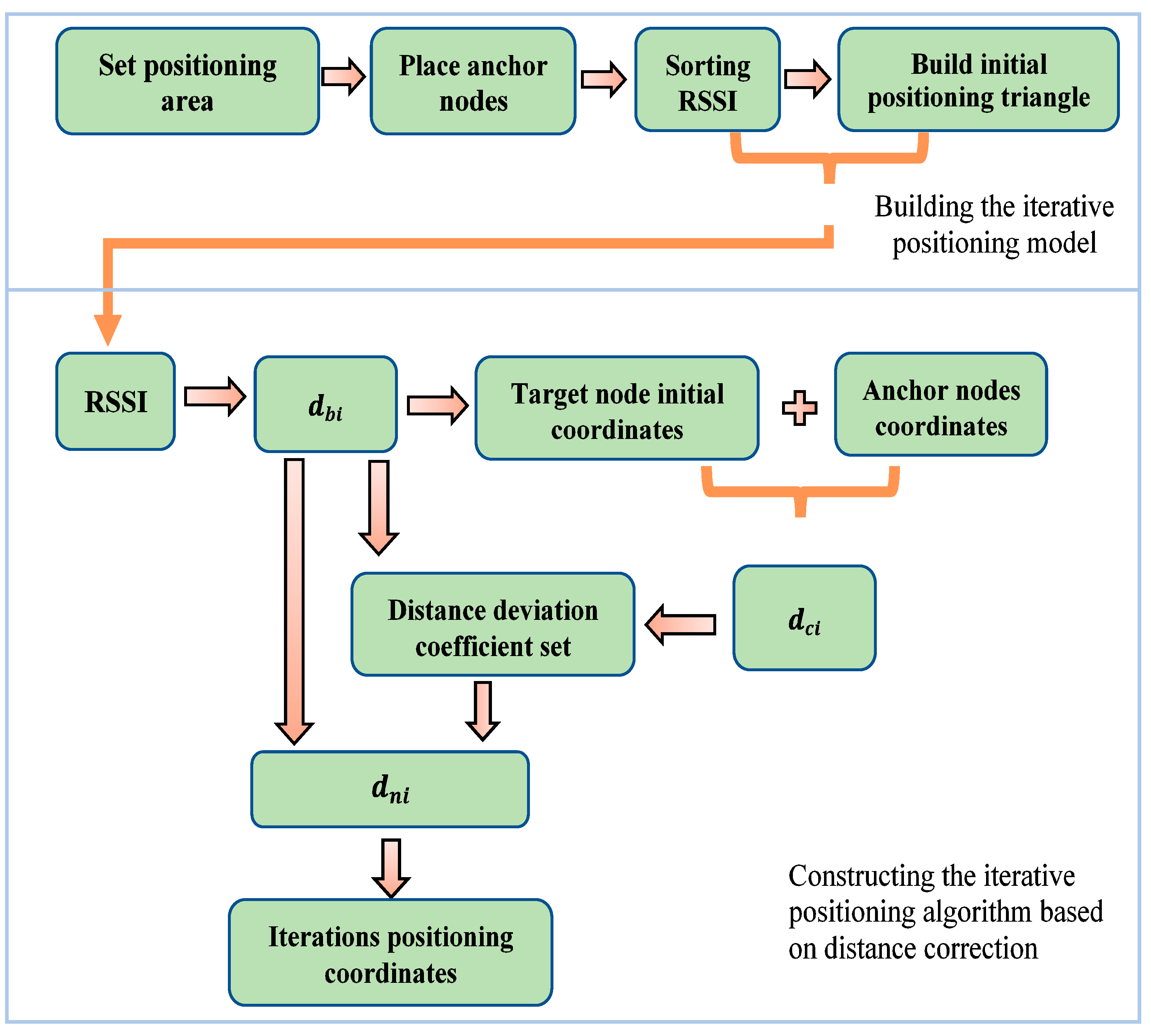
Based on the three issues mentioned above, we propose a target node iterative positioning algorithm based on distance correction in this paper. The motivation of this paper is to reduce the positioning error of the target node to support users to retrieve accurate position information. The process of our target node iterative positioning model based on distance correction is shown in
Figure 1.
In the proposed algorithm, the median of the distance deviation coefficients is used to modify the measured distance during each iteration. The median of the distance deviation coefficients can more closely express the overall distance deviation characteristic. The log-distance distribution model is applied to calculate the distances among unknown target nodes and connected anchor nodes to fit more accurately the nonlinear relationship between distance and RSSI, reducing computational complexity as well. The iterative positioning model is constructed to ensure that the target node is in the region surrounded by its connected anchor nodes, which is also of great help to improving the positioning accuracy. Additionally, the node iterative positioning algorithm based on distance correction can provide theoretical support for future research. Contributions are included in the following aspects.
- (1)
Derivation of noise impact factor based on a log-distance distribution model
The expression of the noise impact factor FN is derived by reconstructing the mathematical model, which is the corresponding numerical relationship between the noise impact factor FN and the measured distance. The noise impact factor derived in this paper is used to describe the influence degree of noise on the measured values of RSSI.
- (2)
The selection of distance deviation coefficient on node measured distance
The distance deviation coefficient is used to evaluate the deviation degree of the distances calculated by the log-distance distribution model and the triangle centroid algorithm, respectively, and a distance deviation coefficients set is established. The median of the distance deviation coefficient set is selected to characterize the measured distance deviation of all nodes, which can better reflect the overall distance deviation characteristic.
- (3)
Construction of the iterative positioning algorithm based on distance correction
The distance deviation coefficient median is used as an iteration factor for the iterative positioning algorithm. In the process of each iteration, the median of the distance deviation coefficients is used to correct the distance from the last positioning, obtaining a distance value closer to the real value. The triangle centroid localization algorithm is iteratively applied to reduce the positioning fluctuation error and improve positioning accuracy.
The rest of this paper is organized as follows. A brief review of related works is presented in
Section 2, while the proposed iterative positioning algorithm is introduced in
Section 3. The iterative positioning model is constructed in
Section 4, the experimental results and corresponding analyses are given in
Section 5, and, finally, conclusions and general discussions are summarized in
Section 6.
2. Related Work
This section reviews two existing works that are the reference foundation theories for the positioning of the target node in WSN. The former is the measurement of the distance between the target node and the anchor node while the latter is to determine the position coordinates of the unknown target node.
2.1. The Measurement of the Distance between the Target Node and the Anchor Node
The measurement of the distance between the target node and the anchor node is an important research topic of the node positioning in WSN. Nowadays, most of the existing node positioning algorithms can be divided into two categories according to whether distance measurements are required or not. One is the range-based measurement positioning algorithm and the other is a range-free measurement positioning algorithm [
14]. The distance measurement refers to calculating the distance between the unknown target node and the given anchor node connected to it through communication between them [
15,
16]. The classic distance measurement algorithms include the algorithm based-TOA (time of arrival), the algorithm based-TDOA (time difference of arrival) [
17], the algorithm based-AOA (angle of arrival) [
18] and the algorithm based-RSSI [
19,
20].
In the above distance measurement algorithms, the first three algorithms (TOA, TDOA, and AOA) need to calculate the distance between the unknown target node and given anchor node accurately by using an algorithm with high complexity that requires not only additional hardware equipment but also excellent node energy consumption. All these significantly increase the communication cost and energy consumption of the positioning process. Hence, the algorithm based-RSSI is adopted to measure distance in the paper for fitting the principle of low power consumption and low cost.
2.2. The Target Node Positioning Algorithm
The target node positioning algorithm can be built in several ways. A triangle centroid positioning (TCP) algorithm based on the distance or relative angle information between the target node and the anchor node has been proposed in the existing documents [
21,
22,
23]. Since the node distribution characteristics are not fully considered, the problems in the TCP algorithm are twofold: the target node deviating active locating area and the significant positioning error. The weighted centroid positioning (WCP) algorithm has been presented in the existing literature [
24,
25,
26,
27] by introducing a weight factor, which is related to the distance estimation. Nevertheless, the positioning error will be significantly enlarged if there is a significant deviation in the distance estimating process of the WCP algorithm. A fingerprint database positioning algorithm has been constructed to improve the positioning accuracy in the existing literature [
28,
29,
30] by collecting the positioning samples in advance. The positioning algorithm highly relies on fingerprint database data and the positioning accuracy will become weak if the environment changes. A positioning algorithm based on the neural network has been put forward in the literature where [
31,
32] the input of the algorithm is the value of RSSI and the output is the distance between nodes. Due to simple learning rules, the output of the neural network cannot be correct when the data is not sufficient. A positioning algorithm based on Bounding-Box has been proposed in the existing literature [
33,
34]. The number of given anchor nodes determines the positioning accuracy of the algorithm and the positioning accuracy is not high if the number of anchor nodes is not enough.
Aiming to address the above problems of low positioning accuracy, several experts have presented the solution of cooperative positioning. A cooperative positioning method fusing inertial-measurement unit and UWB ranging measurement is presented in [
35] and a cooperative positioning method combining the inertial-measurement unit with long-range WiFi RSS and short-range UWB ranging measurements is proposed in [
36] which significantly improves positioning accuracy. However, cooperative positioning methods need additional equipment. For positioning accuracy and low cost, an iterative positioning algorithm based on distance correction is proposed through correcting the estimated distance between the given anchor node and the target node and constraining the target node in the sub-triangular positioning area of the iterative positioning model in this paper. The algorithm calculates the target node coordinates iteratively and improves positioning accuracy effectively.
3. Iterative Positioning Algorithm for the Target Node Based on Distance Correction
An iterative positioning algorithm for the target node based on distance correction is proposed to help users overcome the influence of noise on positioning accuracy. The main issues presented in this paper for building an iterative positioning algorithm based on distance correction are threefold. First, a log-normal distribution mathematical model should be constructed to measure RSSI, based upon which the impact factor of noise on distance detecting can be derived. Second, a triangle centroid positioning algorithm should be built to determine the initial positioning coordinates of the unknown target node, and lastly, the distance deviation coefficient and its median can be determined. Therefore, the iterative positioning algorithm for the target node based on distance correction is constructed according to the median of the distance deviation coefficient.
3.1. Basic Concept
Definition 1. WSN node positioning. WSN node positioning refers to when the position of the unknown target node is calculated based on the communication between the anchor nodes whose position information is known in the network by specific techniques, algorithms, and schemes [37]. Definition 2. Anchor node. The anchor node is the node whose coordinates or position information is known in WSN [38]. Definition 3. Target node. The target node refers to the node whose coordinates or positioning information is unknown in the WSN [39]. 3.2. The Preprocessing of the Iterative Positioning Algorithm
Before the design of the iterative positioning algorithm, some pre-processing tasks must be performed. First of all, the mathematical model of the RSSI is constructed and used to calculate the initially measured distance. Then, the influence of noise on the measured distance is analyzed and thereby the noise impact factor is derived. Finally, the triangle centroid positioning algorithm is used to obtain the initial positioning coordinates of the target node.
3.2.1. RSSI Ranging Algorithm
The concept of the RSSI ranging algorithm is to calculate the distance between the transmitting signal node and the receiving signal node by measuring the received signal strength, since there is a varying degree of losses in the propagating process of wireless signals. Therefore, it is imperative to build an appropriate RSSI ranging model. At present, the model used commonly is the log-distance distribution model [
40,
41,
42,
43].
Pd is used to indicate the power measurement corresponding to the distance between two nodes, denoted
d.
Pd0 is used to indicate the power measurement corresponding to the distance between two nodes, denoted
d0. The relationship between
Pd and
d can be expressed as
where
n is a signal propagation factor, which is usually obtained by empirical value or actual calibration.
The logarithmic processing is performed on both sides of Equation (1), and after arranging, Equation (2) can be obtained as
The relationship between RSSI value and power can be expressed as
Thus, a mathematical model of RSSI ranging can be obtained as
where
P(
d) is the RSSI value when the distance between two nodes is
d and
P(
d0) is the RSSI value when the distance between two nodes is
d0.
3.2.2. The Effect of Noise on RSSI Ranging
The loss of wireless signals during propagation has a significant influence on the accuracy of the RSSI ranging algorithm and must be considered in practical applications. Next we will analyze the effect of signal propagation loss on RSSI ranging. In Equation (4), the measurement value P(d) is composed of the true signal strength value and the noise signal strength value, which are denoted PT(d) and PN(d), respectively. P(d0) is the RSSI value when the distance between the two nodes is d0. To simplify the calculation, d0 is usually taken as 1 and P(d0) is denoted as A.
Thus, the actual mathematical model of the log-distance distribution model is
From Equation (5), the distance between two nodes can be calculated as
Equation (6) can be calculated as follows by further mathematical transformation, i.e.,
Assume that , .
Equation (7) can be expressed as
Equation (8) can be expanded further as
Assuming that
,
, the calculation of distance
d can be simplified to
where
is the real distance between the given anchor node and unknown target node and
is the impact factor of noise on distance measurement.
FN is designated the noise impact factor.
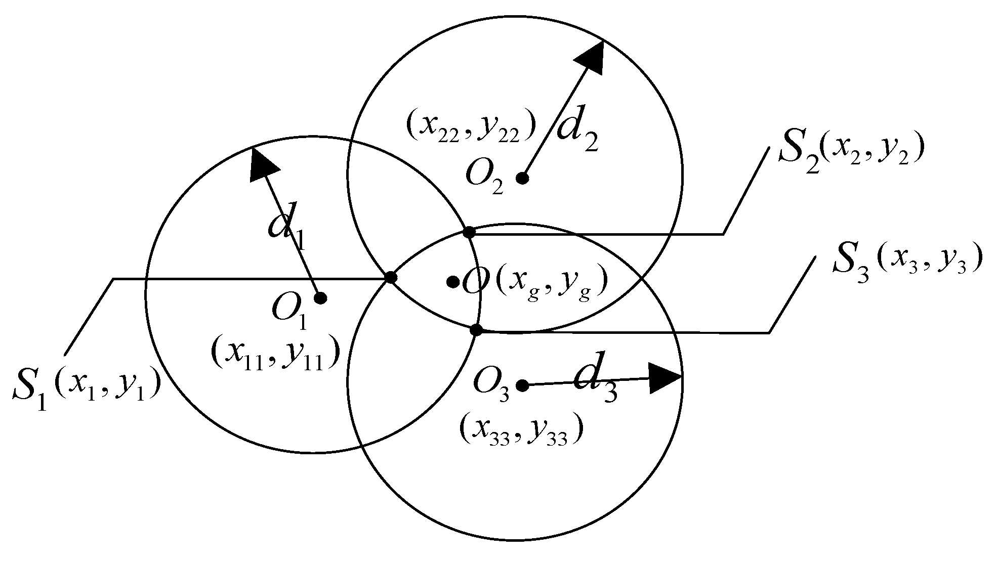
3.2.3. The Triangular Centroid Positioning Algorithm
The basic principle of the triangle centroid positioning algorithm is as follows: the three circles are determined by treating the three anchor nodes as their respective circle centers by addressing the distances between the given anchor nodes and unknown target node as their respective radiuses. The intersection of the three circles can obtain six intersection points and a triangle is constructed by treating the three closer intersection points as vertexes, with the centroid of a triangle taken as the coordinates of the node to be positioned. The schematic diagram of triangular centroid positioning is shown in
Figure 2.
In
Figure 2,
O1,
O2 and
O3 are defined as the positions of three anchor nodes with coordinates of
O1(
x11,
y11),
O2(
x22,
y22), and
O3(
x33,
y33) and whose radiuses are
d1,
d2, and
d3, respectively. Points
S1(
x1,
y1),
S2(
x2,
y2), and
S3(
x3,
y3) are the three closer intersections points, that is, the three vertices of the triangle centroid positioning algorithm.
The intersection point coordinates of the circles O1 and O2 can be obtained by Equation (11).
In two sets of coordinates solved by Equation (11), the intersection S3 (x3, y3) is closer to the center of the positioning triangle. The solution of the remaining points S1(x1, y1) and S2(x2, y2) is similar to that of point S3(x3, y3).
Thus, the initial coordinates
O(
xg,
yg) of the target node can be calculated by Equation (12).
where
m = 3 and
i = 1, 2, 3.
3.3. The Iterative Positioning Algorithm
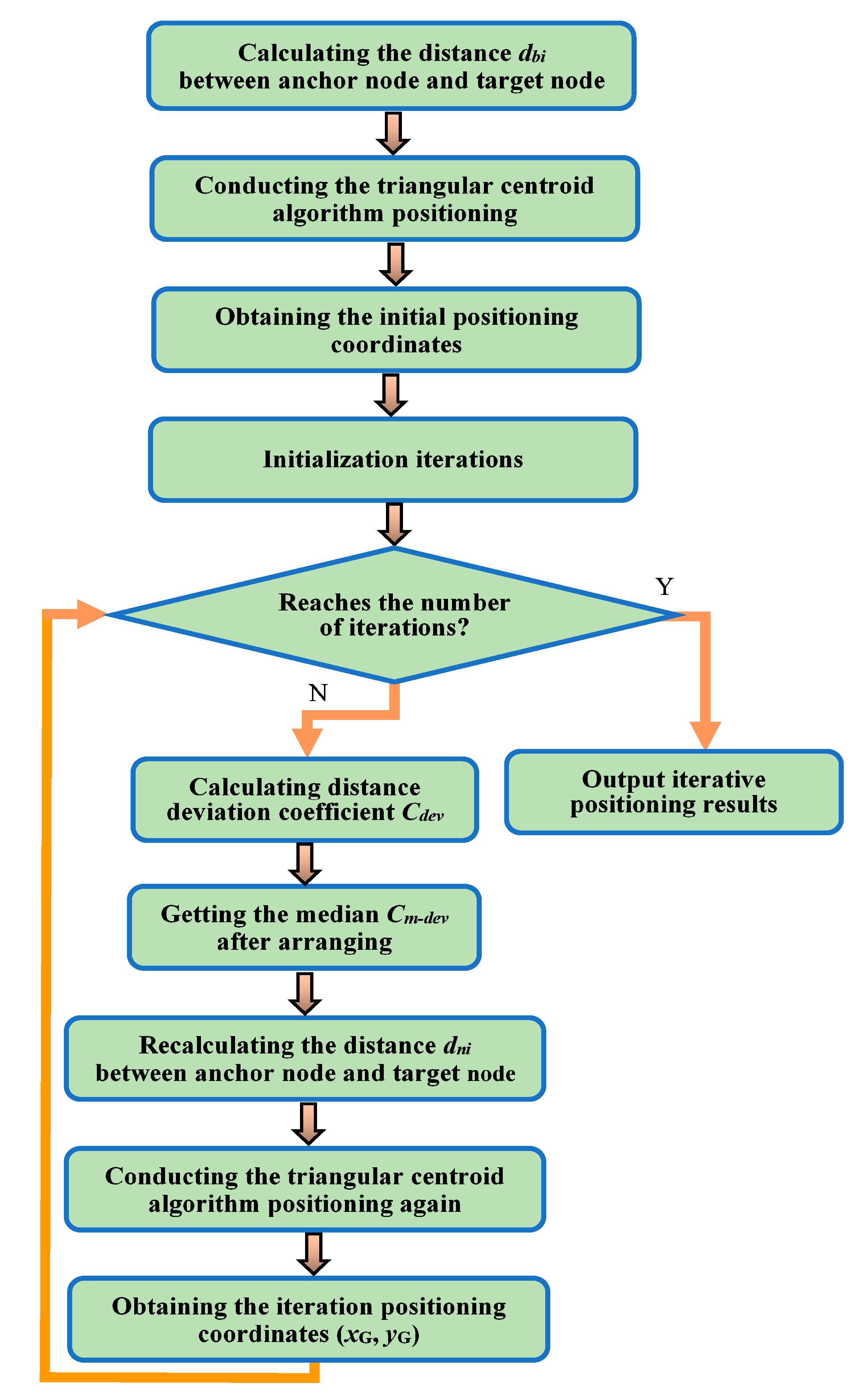
In the actual physical environment, signals are easily disturbed by noise in the transmission process. Therefore, there is a large deviation between the distance obtained by the log-distance distribution model and the real distance value. To further reduce the positioning error, a node iterative positioning algorithm based on distance correction is introduced.
The basic principle of the iterative positioning algorithm based on distance correction is as follows: the distance deviation coefficient is introduced to evaluate the degree of deviation of the distance measured by the log-distance distribution model and the triangle centroid positioning algorithm, respectively. The distance between the given anchor node and the unknown target node is recalculated based on the distance deviation coefficient. By constantly updating the distance between the given anchor node and the unknown target node, the target node coordinates are iteratively calculated.
3.3.1. The Calculation of the Distance Deviation Coefficient
The distance between the given anchor node and unknown target node, which is calculated by the log-distance distribution model, is denoted dbi. The distance between the coordinates of the anchor node and the coordinates calculated by the triangle centroid positioning algorithm is denoted dci. To indicate the deviation of the two distances, the distance deviation coefficient Cdev is defined by Equation (13).
As distance deviation coefficients can be solved by Equation (13), it is essential to determine a characteristic quantity to represent the degree of deviation of the overall node measurement distance. The two statistical parameters, the average value and the median of distance deviation coefficients, can be closely used to express the overall distance deviation characteristics.
The average value of the distance deviation coefficients can express the average level of the overall measurement distance deviation. However, its fatal disadvantage is that if the extremum at both ends is too low or too high, the final calculation result will significantly deviate from the real situation.
Therefore, the median distance deviation coefficients are usually used to express the overall distance deviation characteristics. The median is not affected by the extreme values of both ends and can better reflect the overall distance deviation characteristics, making the final calculation result closer to the real situation.
The distance deviation coefficients are calculated by Equation (13). Then, the values of Cdev are sorted to obtain the median named Cm-dev.
The distance between the given anchor node and unknown target node can be recalculated based on the median Cm-dev, as shown in Equation (14).
The new distance dni is obtained by Equation (14) and the triangular centroid positioning algorithm is iteratively conducted to obtain the positioning result (xG, yG).
3.3.2. The Iteration Termination Criteria for the Algorithm
If the termination condition of the iterative positioning algorithm is set correctly, the higher positioning accuracy can be obtained within a small number of iterations and the algorithm is prevented from falling into an infinite loop. That is, the iteration termination condition is defined as
where
is the RSSI value between the centroid of the
nth iteration and the unknown target node, and
ε is the set threshold.
Under different environmental conditions, as Equation (15) is used as the iterative termination condition, its computational complexity is very high, even higher than the complexity of the iterative positioning algorithm itself. In this way, the hardware complexity of the system increases significantly and the algorithm becomes almost infeasible.
The purpose of iterative positioning is to make the positioning error converge to the expected value, as the convergence property and convergence velocity are essential issues of the iteration. In the process of iteration, with the increased number of iterations, the convergence processes in which the error converges to the expected value usually have the following cases: fast convergence, slow convergence, and periodic oscillation. In order to further study the convergence property of the above three cases, a series of simulations are conducted to analyze the relationship between the positioning error and the number of iterations in the paper. Through simulation analysis, it can be noted that the iterative error varies with the above different regular patterns when the number of iterations is between 0–10 since the iteration error no longer varies when the number of iterations is between 10–20. A flow chart of the iterative positioning algorithm is shown in
Figure 3.
4. The Construction of the Iterative Positioning Model
In the procedure of iterative positioning, the unknown target node in the positioning triangle area has a significant influence on its positioning accuracy. The positioning error of the target node located in the positioning triangle area is much smaller than that of the target node outside the positioning triangle area. To improve the positioning accuracy, an iterative positioning model is established in the paper, as shown in
Figure 4.
In
Figure 4, the quadrilateral
A1A2A3A4 is a square, the point
O is its center, and the points
B1,
B2,
B3, and
B4 are the midpoints of the respective sides. According to the connection shown in
Figure 4, the square
A1A2A3A4 is subdivided into eight triangular regions: region 1 to region 8. The anchor nodes (9 in total) are placed at points
A1,
A2,
A3,
A4,
B1,
B2,
B3,
B4, and
O.
There is a target node
X in the quadrilateral
A1B1OB4 in
Figure 4 and the points closest to the point
X are points
A1,
B1,
O, and
B4 in turn. The node X is included in both Δ
A1B1B4 and Δ
A1B1O. In Δ
A1B1B4, the coordinates (
xG1,
yG1) are calculated by the iterative positioning algorithm. In order to reduce effectively the positioning error caused by noise, the other coordinate (
xG2,
yG2) is calculated by the iterative positioning algorithm in Δ
A1B1O. The weighted average of these two coordinates can be taken as the final coordinates (
xG3,
yG3). The closer the distance between the given anchor node and the unknown target node is, the more reliable the calculation result is. Hence, the weight of the former coordinate should be higher than the weight of the latter coordinate.
Simulation experiments compare the various proportion of weight values and the results show that when the weight of the former coordinate is 0.75 and the weight of the latter coordinate is 0.25, the positioning result is better than others.
The final positioning results can be expressed as follows in Equation (16).
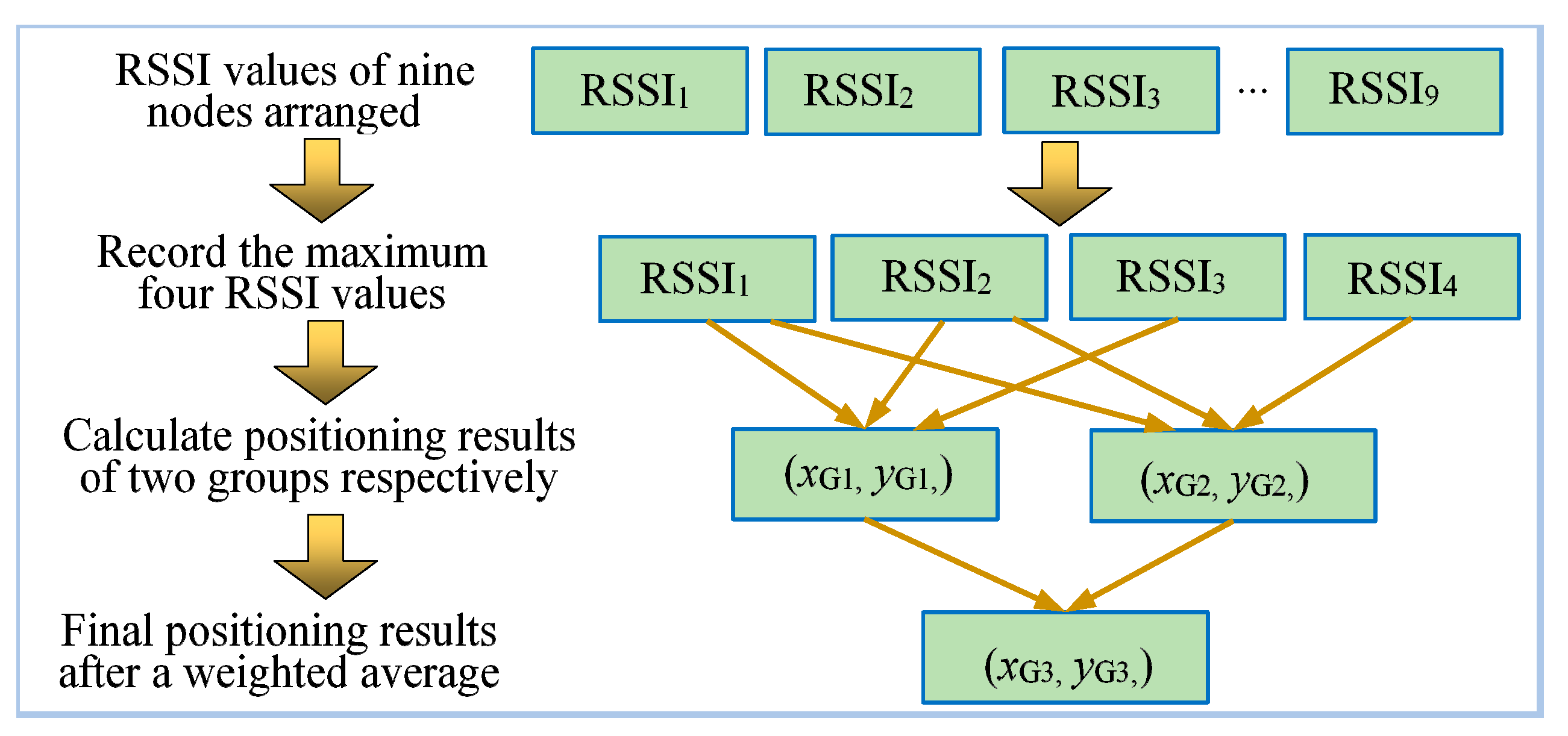
In actual positioning progress, the RSSI values of the nine anchor nodes are recorded and arranged in descending order. The first four larger RSSI values are denoted RSSI1, RSSI2, RSSI3, and RSSI4. The primary positioning coordinate (xG1,yG1) is calculated by RSSI1, RSSI2, RSSI3 and their corresponding coordinates. The second positioning coordinate (xG2,yG2) is calculated by RSSI1, RSSI2, RSSI4, and their corresponding coordinates. The weighted average of two coordinates according to the weights mentioned above is the final positioning result (xG3,yG3).
The positioning process of the iterative positioning algorithm is shown in
Figure 5.
5. Experimental Results
5.1. The Method
To accurately and quantitatively verify the performance of the iterative positioning algorithm proposed, the experimental positioning area is set as a square of 40 m × 40 m with nine anchor nodes located at the vertices, center, and in the middle of the edges of the square. Now, 50 target nodes are generated in the square area by random and their positioning results calculated in turn.
In this experiment, for different noise impact factors FN, positioning error is discussed by three methods, namely, the centroid positioning algorithm, the weighted centroid positioning algorithm, and the iterative positioning algorithm based on distance correction. The value of FN is taken into account in two situations: that involving a constant value and that involving a random value.
5.2. Experimental Analysis
According to the above experimental method, two experiments were conducted.
5.2.1. The First Experiment: FN is Constant
When FN is a constant value, considering the effects of the actual noise on the signal, three typical FN values are used for the experiments, these being 0.1, 0.2, and 0.3, respectively.
The experiments for the three parameters are shown as follows.
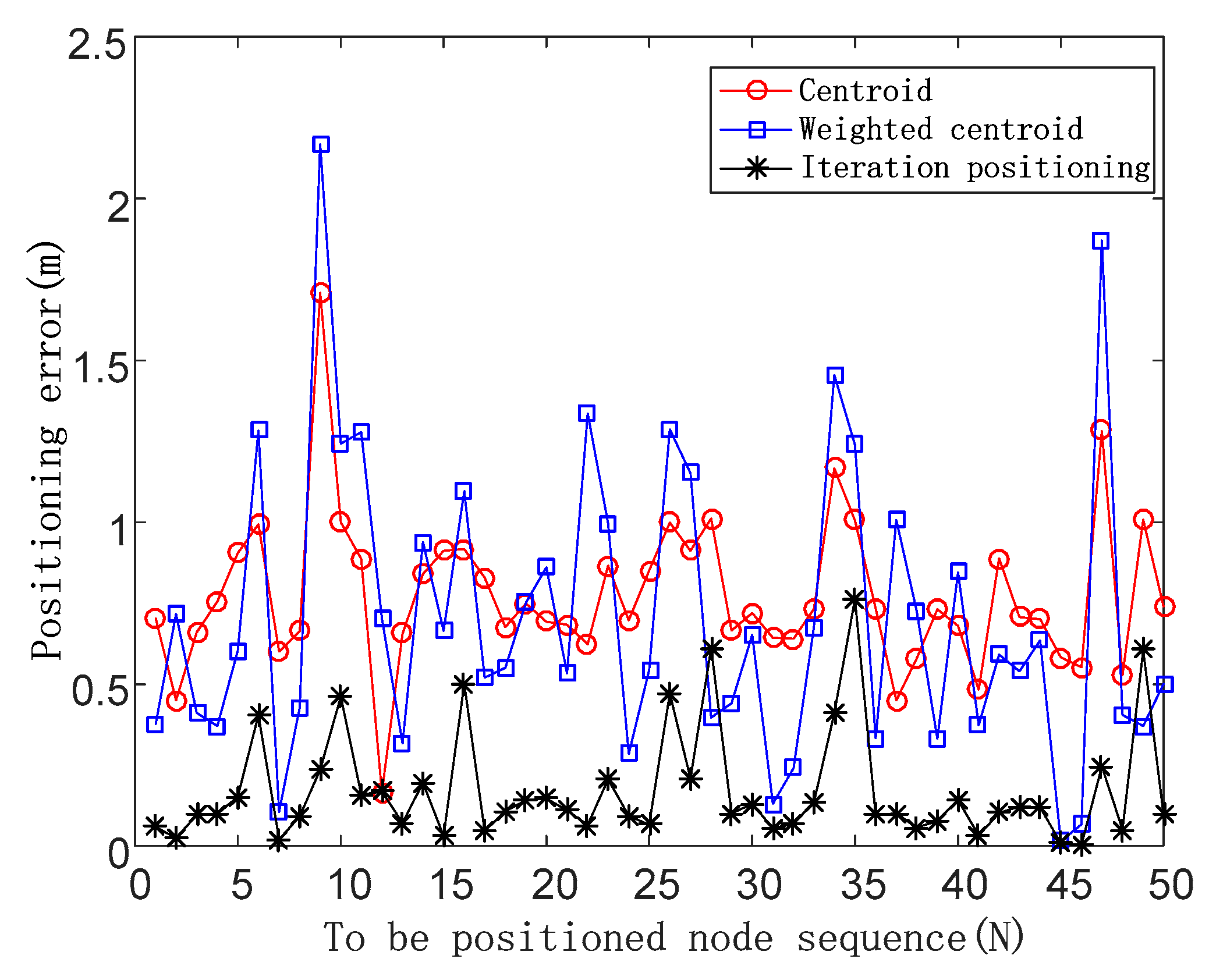
The positioning errors are shown in
Figure 6 in the case of the noise impact factor of 0.1.
The x-coordinate represents the target node sequence, the unit is the number of nodes, and the y-coordinate represents the positioning error, with the unit being m (meters).
When FN is 0.1, the average positioning errors of the three algorithms are 0.77, 0.70, and 0.17, respectively, and the positioning accuracy of the iterative positioning algorithm is improved by 77.92% and 75.71% compared with the centroid algorithm and the weighted centroid algorithm.
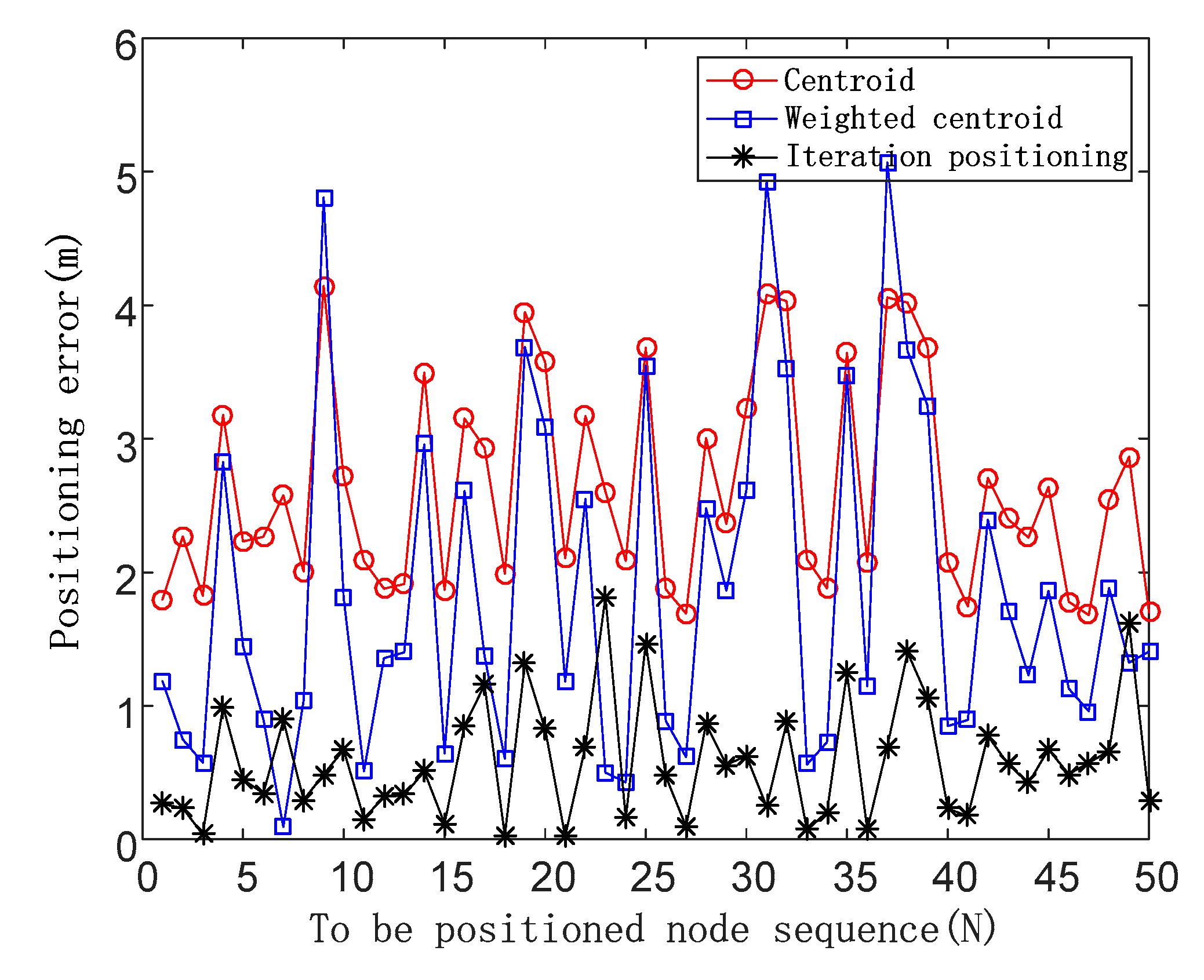
The positioning errors are shown in
Figure 7 in the case of the noise impact factor of 0.2.
When FN is 0.2, the average positioning errors of the three algorithms are 1.68, 1.30, and 0.42, respectively, and the positioning accuracy of the iterative positioning algorithm is improved by 75% and 67.69% compared with the centroid algorithm and the weighted centroid algorithm.
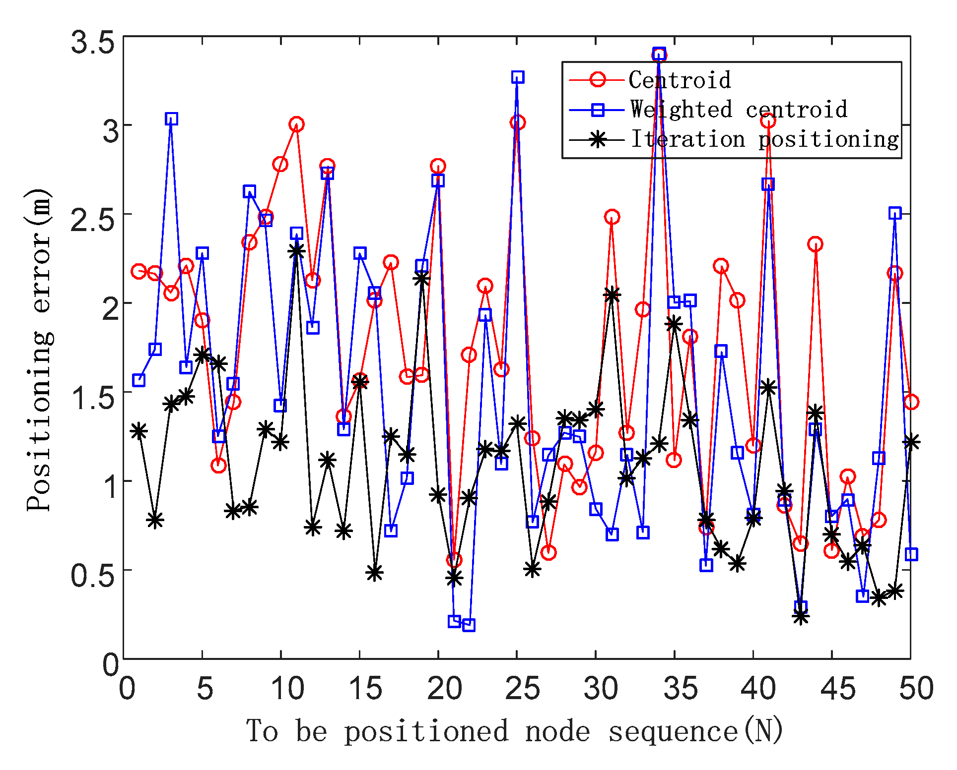
The positioning errors are shown in
Figure 8 in the case of a noise impact factor of 0.3.
When FN is 0.3, the average positioning errors of the three algorithms are 2.63, 1.85, and 0.79, respectively, and the positioning accuracy of the iterative positioning algorithm is improved by 69.96% and 57.29% compared with the centroid algorithm and the weighted centroid algorithm.
5.2.2. The Second Experiment: FN Is a Random Value
When FN is an arbitrary value, considering the effect of the actual noise on the signal, the random value is 0.3 times that of the random function.
The positioning errors are shown in
Figure 9 in the case of the noise impact factor of a random value.
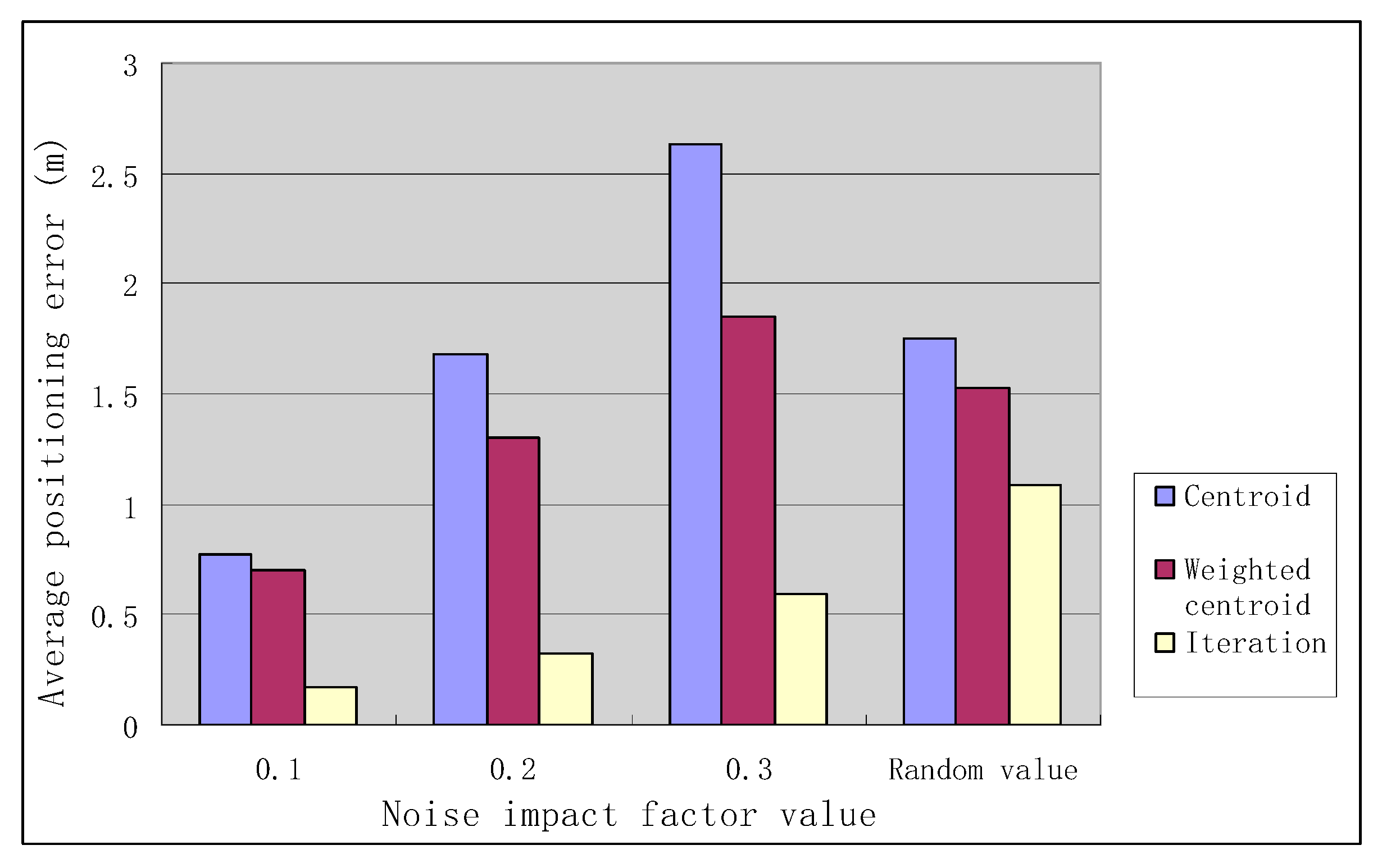
In the case of different noise impact factors, the positioning errors of the three positioning algorithms are shown in
Table 1.
As can be seen from
Table 1, when
FN is constant, the positioning accuracy decreases with the increase of
FN, i.e., the noise has more and more influence on the positioning accuracy; when
FN is a random value, the positioning accuracy of the iterative positioning algorithm is improved by 37.71% compared with the centroid algorithm and the positioning accuracy of the iterative positioning algorithm is improved by 28.76% compared with the weighted centroid algorithm.
The positioning errors of the three positioning algorithms for different values of noise impact factors are shown in
Figure 10.
As can be seen from
Figure 10, the positioning error of the iterative positioning algorithm is smaller than that of the centroid positioning algorithm and the weighted centroid positioning algorithm in the case of different noise impact factors
FN.
6. Conclusions
With the development of wireless communication technology, the position information of data is playing an increasingly important role. There are errors in node positioning due to various interferences in the data transmission process. As an alternative to this problem, a node iterative positioning algorithm based on distance correction is proposed in this paper to help users obtain accurate position information. Contributions include the following aspects:
- (1)
The noise impact factor FN has been derived based on the original log-distance distribution model, which is used to describe the corresponding relationship between the noise impact factor FN and the measured distance. Proposing a noise impact factor provides a novel method for analyzing the influence of noise on the distance measurement between nodes in WSN.
- (2)
The median of the distance deviation coefficient has been constructed to characterize the deviation degree of the whole measured distances and used to correct the range from the last positioning. The triangle centroid localization algorithm has been iteratively conducted based on the adjusted new distance value to improve the node positioning accuracy.
Experimental results show that the node iterative positioning algorithm based on distance correction can reduce the positioning error of unknown target nodes in wireless sensor networks effectively and help users obtain more accurate node coordinates. In the future, based on the node iterative positioning algorithm proposed in this paper, we will move forward with related research including real-time tracking and path planning of moving nodes in WSNs.
Author Contributions
Conceptualization, J.C., S.W., and K.-C.L.; methodology, all authors; software, J.C., M.O., and K.-C.L.; validation, J.C. and Y.X.; formal analysis, J.C., S.W., and Y.X.; investigation, J.C. and M.O.; resources, J.C., S.W., and K.-C.L.; data curation, S.W., K.-C.L., and Y.X.; writing—original draft preparation, J.C., M.O., and K.-C.L.; writing—review and editing, J.C., S.W., and M.O.; visualization, J.C. and K.-C.L.; supervision, J.C. and K.-C.L.; project administration, J.C. and M.O.; funding acquisition, J.C.
Funding
This research was funded by the Natural Science Foundation of the Education Department of Anhui province (KJ2018A0087) and the Natural Science Foundation of China (51874010).
Conflicts of Interest
The authors declare no conflict of interest.
References
- Yassin, A.; Nasser, Y.; Awad, M.; Al-Dubai, A.; Liu, R.; Yuen, C.; Raulefs, R.; Aboutanios, E. Recent Advances in Indoor Localization: A Survey on Theoretical Approaches and Applications. IEEE Commun. Surv. Tutor. 2017, 19, 1327–1346. [Google Scholar] [CrossRef]
- Pandey, S.; Varma, S.A. Range-Based Localization System in Multihop Wireless Sensor Networks A Distributed Cooperative Approach. Wirel. Pers. Commun. 2016, 86, 615–634. [Google Scholar] [CrossRef]
- Safavi, S.; Khan, U.A. Localization in mobile networks via virtual convex hulls. IEEE Trans. Signal Inf. Process. Netw. 2018, 4, 188–201. [Google Scholar] [CrossRef]
- Benatia, M.A.; Sahnoun, M.; Baudry, D. Multi-Objective WSN Deployment Using Genetic Algorithms Under Cost, Coverage, and Connectivity Constraints. Wirel. Pers. Commun. 2017, 94, 2739–2768. [Google Scholar] [CrossRef]
- Senouci, M.R.; Lehtihet, H.E. Sampling-based selection-decimation deployment approach for large-scale wireless sensor networks. Ad Hoc Netw. 2018, 75–76, 135–146. [Google Scholar] [CrossRef]
- Zhang, S.; Wang, Y.; Zhang, S.; Zhu, G. Building course semantic view for representing course content concisely. Int. J. Comput. Sci. Eng. 2016, 13, 400–409. [Google Scholar] [CrossRef]
- Martino, B.D.; Li, K.C.; Yang, L.T.; Esposito, A. Trends and Strategic Researches in Internet of Everything. In Internet of Everything; Springer: Singapore, 2018; pp. 1–12. [Google Scholar]
- Raja, P.; Dananjayan, P. Game Theory Based Cooperative MIMO Routing Scheme for Lifetime Enhancement of WSN. Int. J. Wirel. Inf. Netw. 2015, 22, 116–125. [Google Scholar] [CrossRef]
- Rai, R.; Rai, P. Survey on Energy-Efficient Routing Protocols in Wireless Sensor Networks Using Game Theory. In Advances in Communication, Cloud, and Big Data; Springer: Singapore, 2019; Volume 31, pp. 1–9. [Google Scholar]
- Halder, S.; Ghosal, A. A survey on mobile anchor assisted localization techniques in wireless sensor networks. Wirel. Netw. 2016, 22, 2317–2336. [Google Scholar] [CrossRef]
- Alletto, S.; Cucchiara, R.; Fiore, G.D. An Indoor Location-Aware System for an IoT-Based Smart Museum. IEEE Internet Things J. 2016, 3, 244–253. [Google Scholar] [CrossRef]
- Zhang, X.R.; Xiong, W.L.; Xu, B.G. A Whole Process Optimization Distributed Localization Strategy Based on RSSI in Wireless Sensor Networks. Chin. J. Sens. Actuators 2016, 29, 1875–1881. [Google Scholar]
- Tomic, S.; Beko, M.; Rui, D. Distributed RSS-AoA Based Localization with Unknown Transmit Powers. IEEE Wirel. Commun. Lett. 2016, 29, 3–395. [Google Scholar] [CrossRef]
- Sahu, P.K.; Wu, E.H.-K.; Sahoo, J. DuRT: Dual RSSI Trend Based Localization for Wireless Sensor Networks. IEEE Sens. J. 2013, 13, 3115–3123. [Google Scholar] [CrossRef]
- Yaghoubi, F.; Abbasfar, A.A.; Maham, B. Energy-efcient RSSI-based localization for wireless sensor networks. IEEE Commun. Lett. 2014, 18, 973–976. [Google Scholar] [CrossRef]
- Li, J.Z.; Ren, P.; Shi, L.L.; Zhang, S.X. Optimisation of moving target’s low-power and high-precision monitoring with RSSI based on static and dynamic clustering. Int. J. Embed. Syst. 2015, 7, 334–344. [Google Scholar]
- Tomic, S.; Beko, M.; Dinis, R. RSS-based localization in wireless sensor networks using convex relaxation: On cooperative and cooperative schemes. IEEE Trans. Veh. Technol. 2015, 64, 2037–2050. [Google Scholar] [CrossRef]
- Hou, Y.; Yang, X.; Abbasi, Q.H. Efficient AoA-Based Wireless Indoor Localization for Hospital Outpatients Using Mobile Devices. Sensors 2018, 18, 3698. [Google Scholar] [CrossRef]
- Zhang, X.H.; Wang, T.J.; Fang, J.L. A node localization approach based on mobile beacon using particle swarm optimization in wireless sensor networks. Int. J. Embed. Syst. 2017, 9, 112–118. [Google Scholar] [CrossRef]
- Ke, C.; Wu, M.; Chan, Y.; Lu, K. Developing a BLE Beacon-Based Location System Using Location Fingerprint Positioning for Smart Home Power Management. Energies 2018, 11, 3464. [Google Scholar] [CrossRef]
- Chowdhury, T.J.S.; Elkin, C.; Devabhaktuni, V.; Rawat, D.B.; Oluoch, J. Advances on localization techniques for wireless sensor networks: A survey. Comput. Netw. 2016, 110, 284–305. [Google Scholar] [CrossRef]
- Sharma, G.; Kumar, A. Improved range-free localization for three-dimensional wireless sensor networks using genetic algorithm. Comput. Electr. Eng. 2018, 72, 808–827. [Google Scholar] [CrossRef]
- Wang, Z.; Zhang, H.; Lu, T.; Gulliver, T.A. Cooperative RSS-Based localization in wireless sensor networks using relative error estimation and semidefinite programming. IEEE Trans. Veh. Technol. 2019, 68, 483–497. [Google Scholar] [CrossRef]
- Zhang, Y.; Xu, X.L.; Xu, K.Y. Algorithm based on weighted centroid method for WLAN indoor positioning. J. Electr. Meas. Instrum. 2015, 29, 1036–1041. [Google Scholar]
- Zhang, S.; Yin, X.; He, C. The automatic estimating method of the in-degree of nodes in associated semantic network oriented to big data. Clust. Comput. 2016, 19, 1895–1905. [Google Scholar] [CrossRef]
- Phoemphon, S.; So-In, C.; Leelathakul, N. Fuzzy Weighted Centroid Localization with Virtual Node Approximation in Wireless Sensor Networks. IEEE Internet Things J. 2018, 5, 4728–4752. [Google Scholar] [CrossRef]
- Shah, S.B.; Chen, Z.; Yin, F.; Khan, I.U.; Begum, S.; Faheem, M.; Khan, F.A. 3D weighted centroid algorithm & RSSI ranging model strategy for node; localization in WSN based on smart devices. Sustain. Cities Soc. 2018, 39, 298–308. [Google Scholar]
- Huo, H.; Yang, H.H.; Zhen, D.Y.; Liu, L.; Zhang, W. Advanced indoor position algorithm based on RSSI fingerprint. Appl. Res. Comput. 2017, 24, 2786–2790. [Google Scholar]
- Fang, X.; Jiang, Z.; Nan, L.; Chen, L. Optimal weighted K-nearest neighbour algorithm for wireless sensor network fingerprint localisation in noisy environment. IET Commun. 2018, 12, 1171–1177. [Google Scholar] [CrossRef]
- Panarat, C.; Pitikhate, S. Soft-clustering Technique for Fingerprint-based Localization. Sens. Mater. 2018, 30, 2221–2233. [Google Scholar]
- Gholami, M.; Cai, N.; Brennan, R.W. An artificial neural network approach to the problem of wireless sensors network localization. Robot. Comput.-Integr. Manuf. 2013, 29, 96–109. [Google Scholar] [CrossRef]
- Saber, B.S.; Fazlollah, A.; Mehdi, S. A New Range-Free and Storage-Efficient Localization Algorithm Using Neural Networks in Wireless Sensor Networks. Wirel. Pers. Commun. 2018, 98, 1547–1568. [Google Scholar]
- Qian, K.G.; Wang, Y.J.; Li, X.M.; Dai, Z.C. An Improved Bounding Box Localization Algorithm Based on Optimum Node Selection. Appl. Mech. Mater. 2014, 668, 1359–1362. [Google Scholar] [CrossRef]
- Wei, Y.; Chen, T.; Li, W. An Indoor Localization Algorithm Based on Dynamic Measurement Compressive Sensing for Wireless Sensor Networks. In Proceedings of the 2015 International Conference on Identification, Information, and Knowledge in the Internet of Things (IIKI), Beijing, China, 22–23 October 2015; pp. 158–162. [Google Scholar]
- Liu, R.; Yuen, C.; Do, T.; Jiao, D.; Liu, X.; Tan, U. Cooperative relative positioning of mobile users by fusing IMU inertial and UWB ranging information. In Proceedings of the 2017 IEEE International Conference on Robotics and Automation (ICRA), Singapore, 29 May–3 June 2017; pp. 5623–5629. [Google Scholar]
- Liu, R.; Yuen, C.; Do, T.; Zhang, M.; Guan, Y.L.; Tan, U.-X. Cooperative positioning for emergency responders using self IMU and peer-to-peer radios measurements. Inf. Fusion 2020, 56, 93–102. [Google Scholar] [CrossRef]
- Sapre, S.; Mini, S. Optimized Relay Nodes Positioning to Achieve Full Connectivity in Wireless Sensor Networks. Wirel. Pers. Commun. 2018, 99, 1521–1540. [Google Scholar] [CrossRef]
- Singh, P.; Khosla, A.; Kumar, A.; Khosla, M. Computational intelligence based localization of moving target nodes using single anchor node in wireless sensor networks. Telecommun. Syst. 2018, 69, 397–411. [Google Scholar] [CrossRef]
- Singh, P.; Khosla, A.; Kumar, A.; Khosla, M. Optimized localization of target nodes using single mobile anchor node in wireless sensor network. Int. J. Electron. Commun. 2018, 91, 55–65. [Google Scholar] [CrossRef]
- Tian, Z.J.; Li, Z.W.; Liu, X.Y. A Positioning Method in Mine Tunnel Based on Joint Electromagnetic Wave and Ultrasonic Distance Measurement. Trans. Beijing Inst. Technol. 2014, 34, 1177–1185. [Google Scholar]
- Zheng, X.L.; Fu, J.Q. Research on Indoor Location Algorithm Based on PDR and RSSI. J. Instrum. 2015, 36, 1177–1185. [Google Scholar]
- Goldoni, E.; Savioli, A.; Risi, M.; Gamba, P. Experimental analysis of RSSI-based indoor localization with IEEE 802.15.4. In Proceedings of the IEEE European Wireless Conference, Lucca, Italy, 12–15 April 2010; pp. 71–77. [Google Scholar]
- Fan, W.; Zhang, H.; Li, K.C.; Zhang, S.; Marino, M.D.; Jiang, H. An efficient algorithm for modeling and dynamic prediction of network traffic. Int. J. Comput. Sci. Eng. 2018, 16, 311–320. [Google Scholar]
© 2019 by the authors. Licensee MDPI, Basel, Switzerland. This article is an open access article distributed under the terms and conditions of the Creative Commons Attribution (CC BY) license (http://creativecommons.org/licenses/by/4.0/).


