A Novel Data Reduction Approach for Structural Health Monitoring Systems


Abstract
1. Introduction
2. The Proposed Data Reduction Method
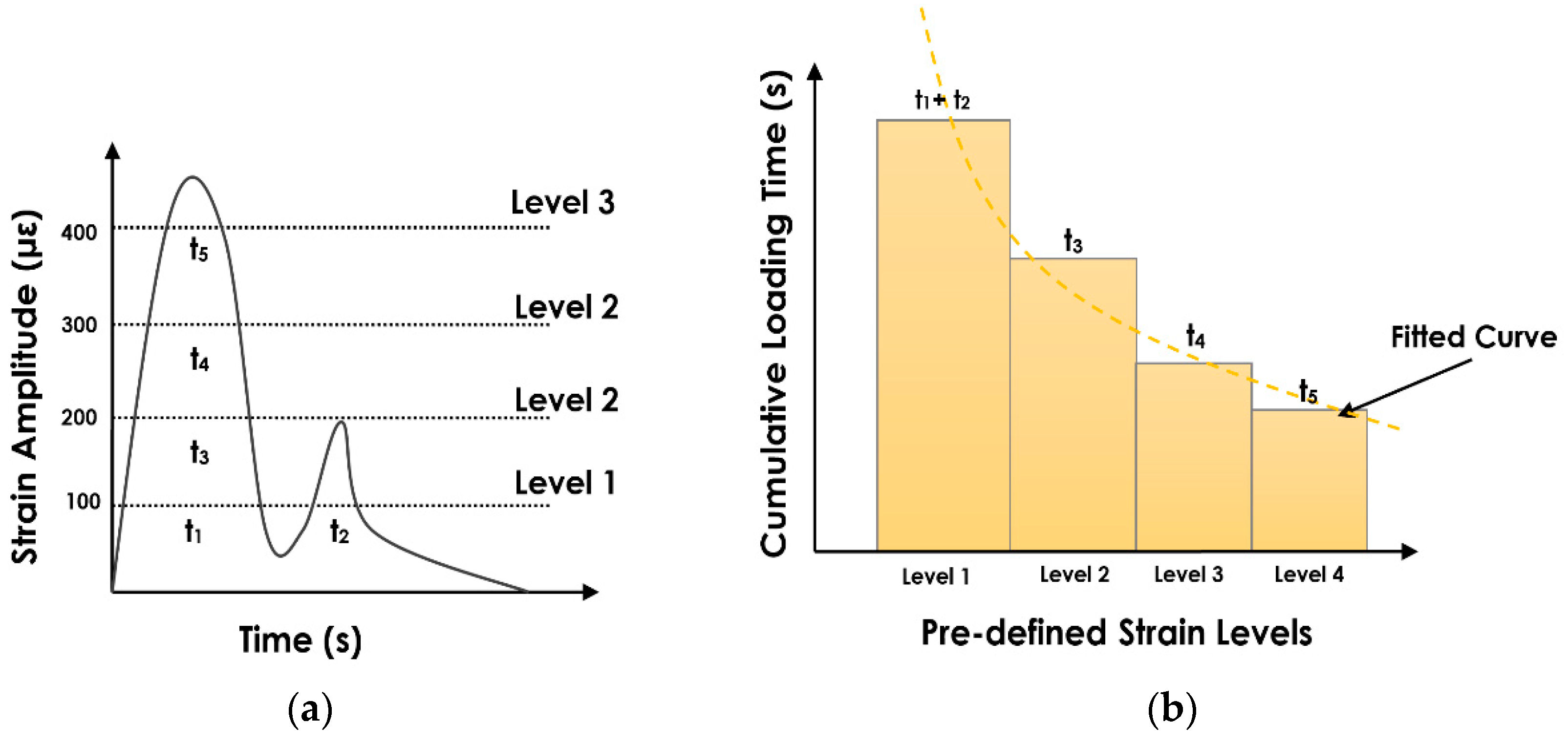
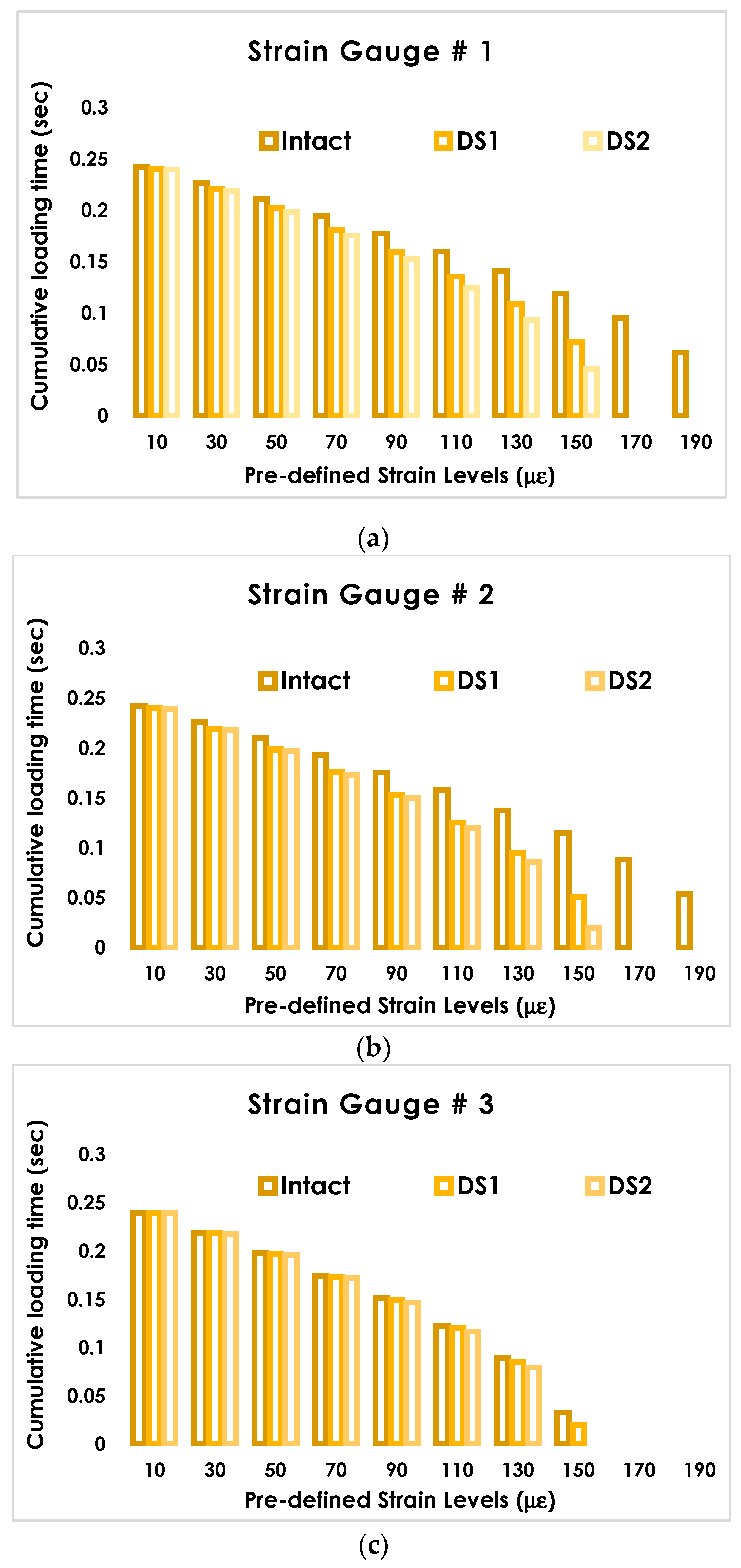
- Measuring the cumulative times at designed levels from the strain signals
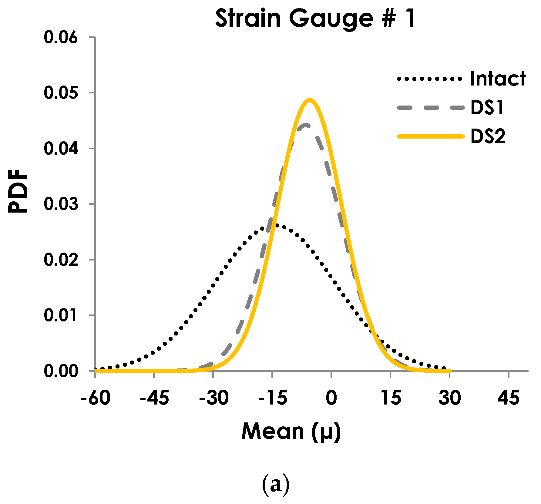
- Fitting a distribution function to the cumulative time histograms
- Calculating the cumulative distribution features for damage detection
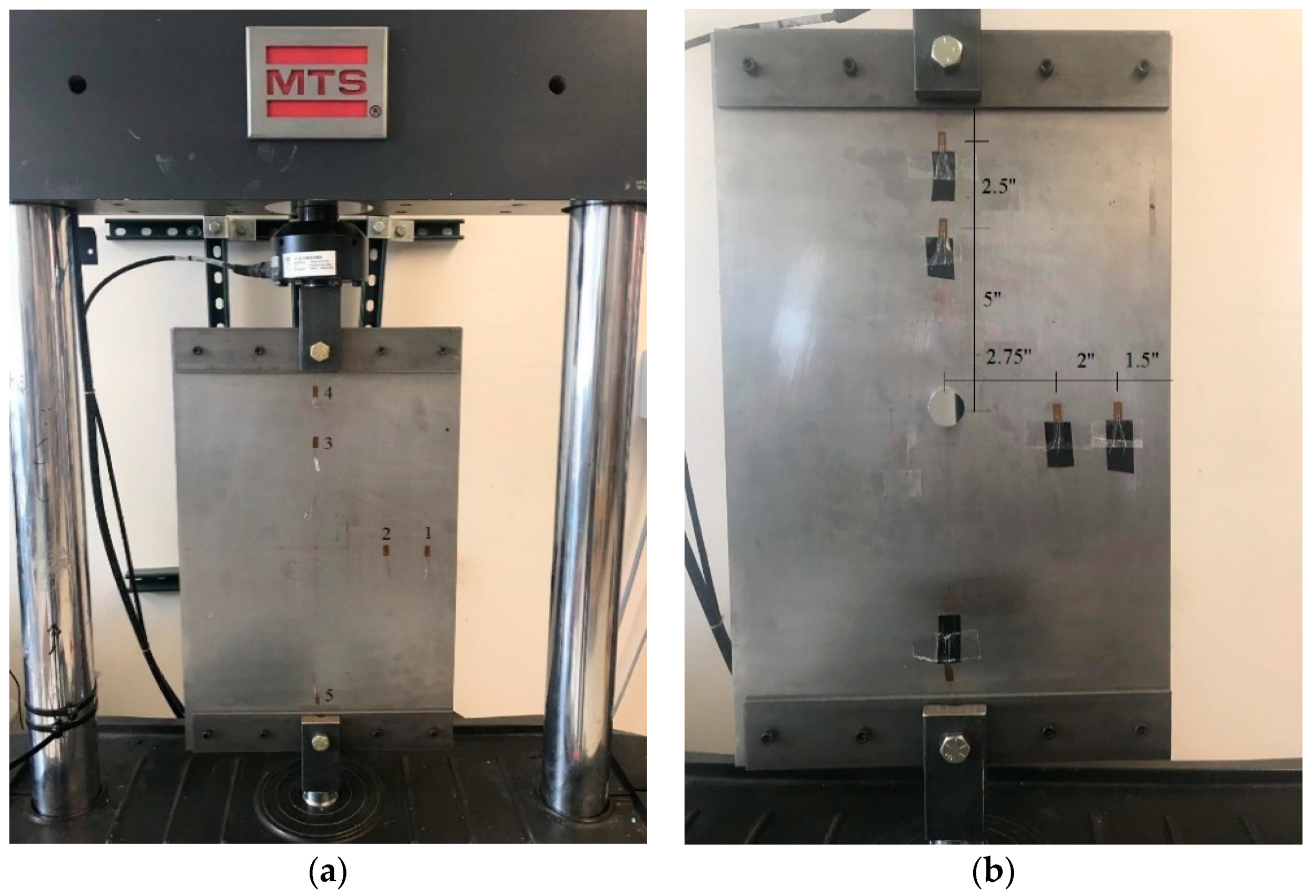
3. Experimental Study
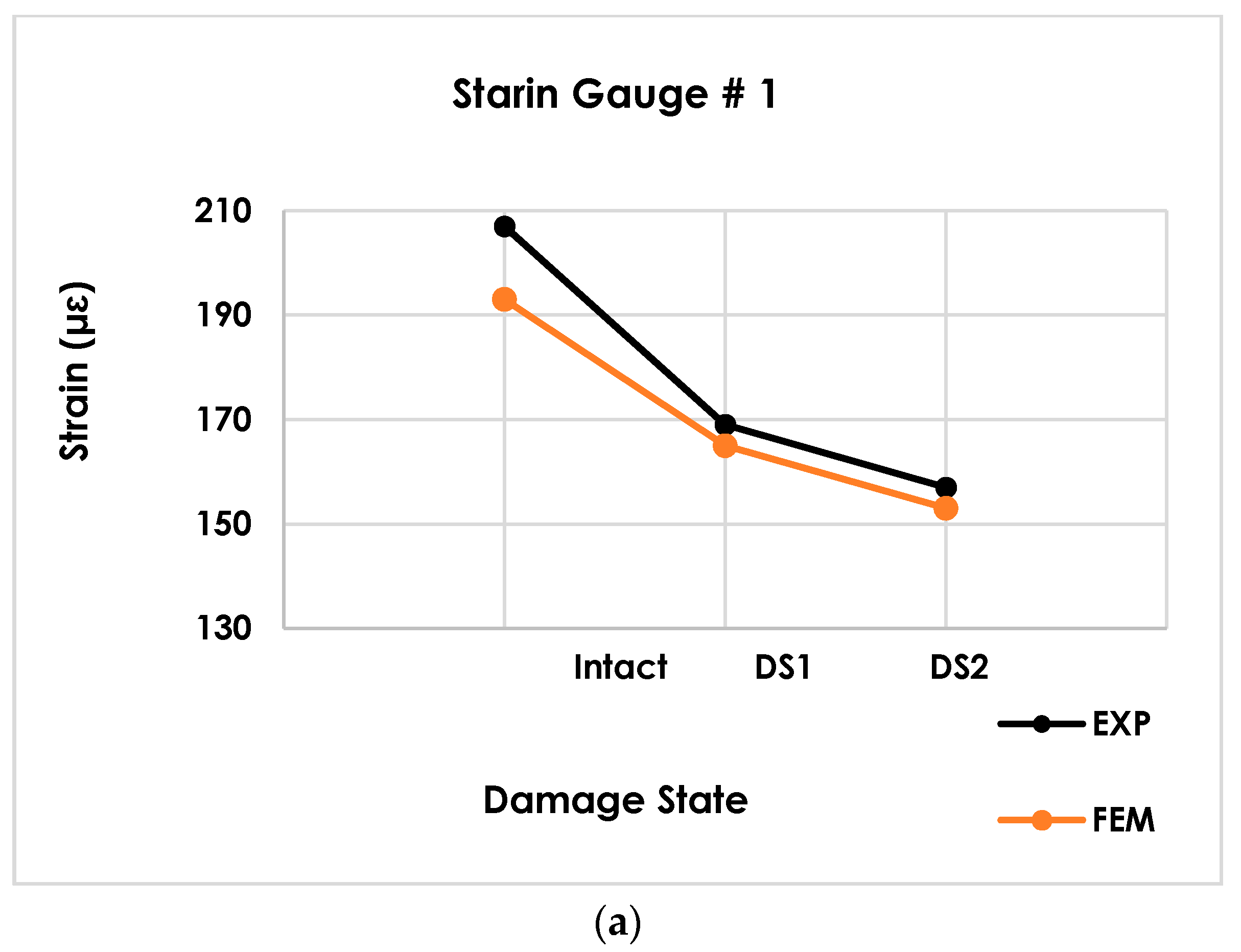
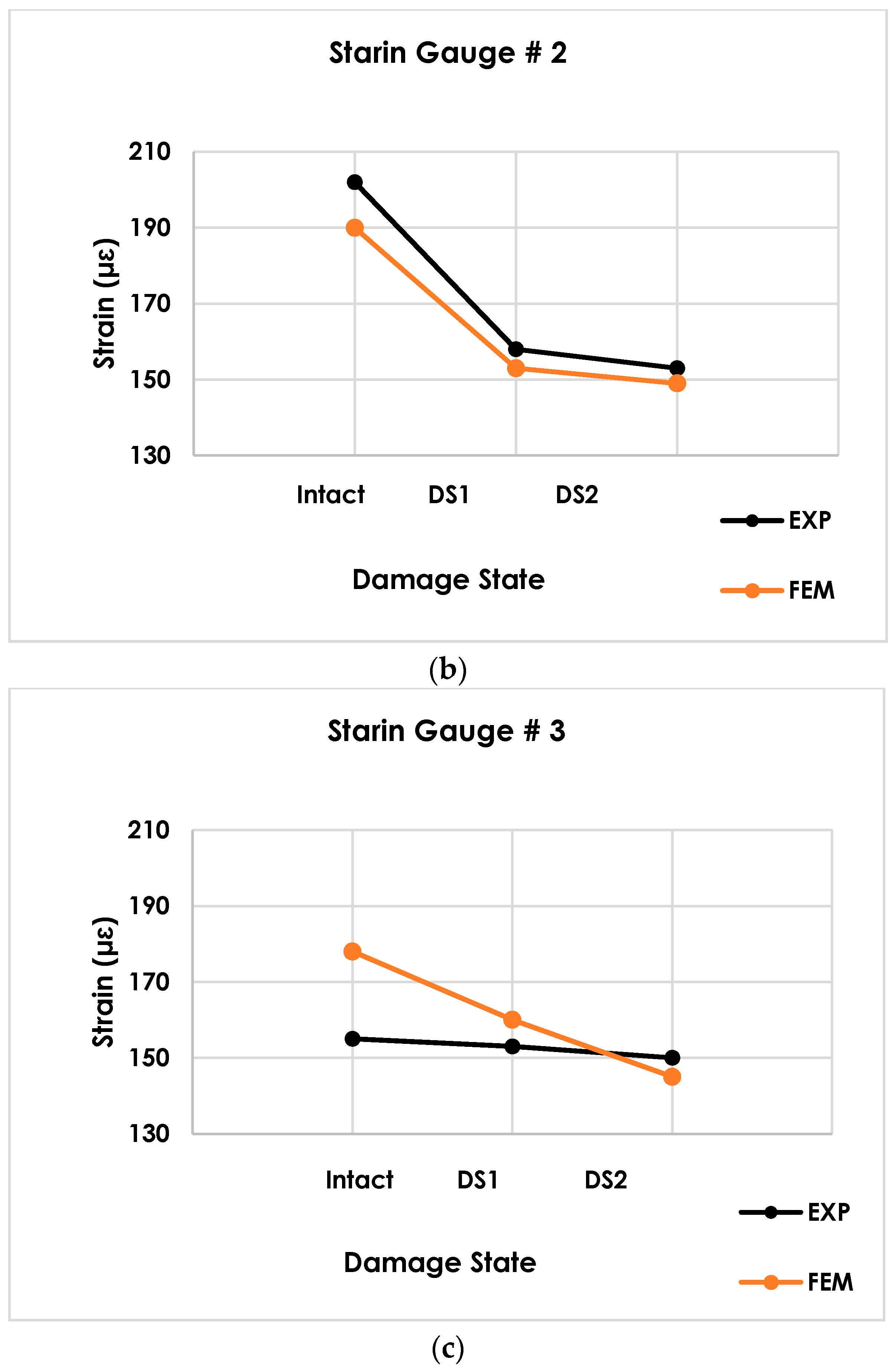
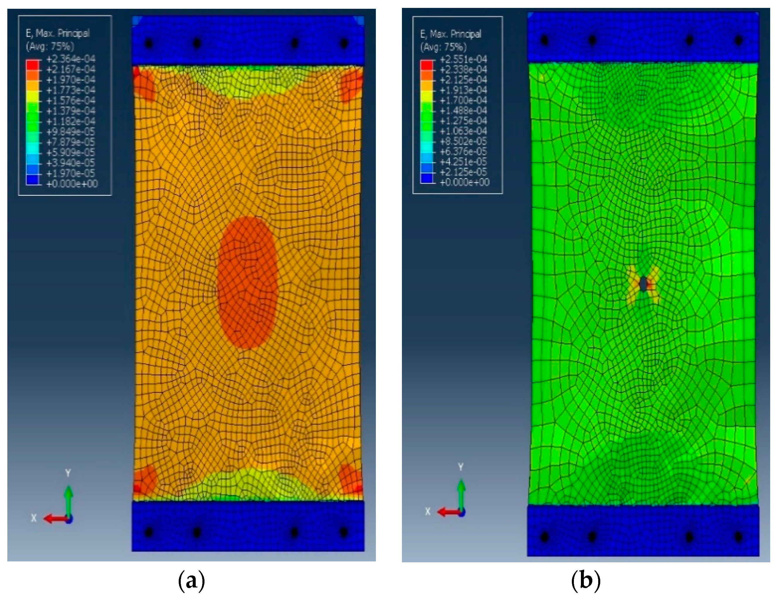
- Intact: D = 0 mm
- Damage state 1 (DS1): D = 12.7 mm (0.5 inch)
- Damage state 2 (DS2): D = 25.4 mm (1 inch)
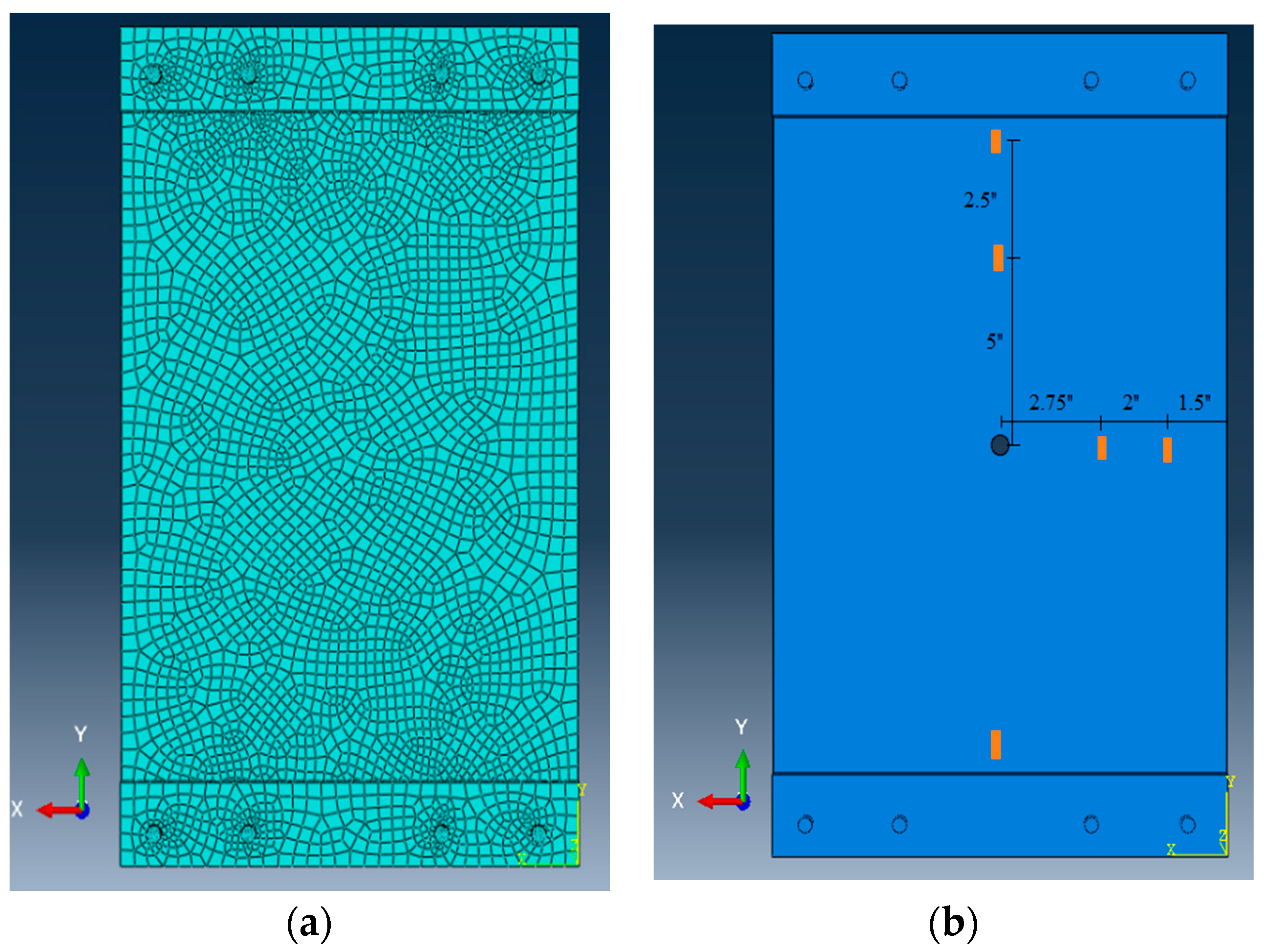
4. Numerical Study
- Total of 3129 C3D8R elements
- Elastic modulus (E) = 200 GPa
- Poisson’s ratio (ν) = 0.3
- Density = 7800 kg/m3.
5. Damage Growth Detection Using the Proposed Data Reduction Method
6. Discussion
7. Conclusions
Author Contributions
Funding
Acknowledgments
Conflicts of Interest
References
- Chang, F.-K. Structural Health Monitoring: Current Status and Perspectives; CRC Press, Inc.: Boca Raton, FL, USA, 1997. [Google Scholar]
- Dos Santos, I.L.; Pirmez, L.; Lemos, É.T.; Delicato, F.C.; Pinto, L.A.V.; De Souza, J.N.; Zomaya, A.Y. A localized algorithm for Structural Health Monitoring using wireless sensor networks. Inf. Fusion 2014, 15, 114–129. [Google Scholar] [CrossRef]
- Flynn, E.B.; Todd, M.D.; Croxford, A.J.; Drinkwater, B.W.; Wilcox, P.D. Enhanced detection through low-order stochastic modeling for guided-wave structural health monitoring. Struct. Health Monit. 2012, 11, 149–160. [Google Scholar] [CrossRef]
- Overbey, L.A.; Todd, M.D. Analysis of Local State Space Models for Feature Extraction in Structural Health Monitoring. Struct. Heal. Monit. 2007, 6, 145–172. [Google Scholar] [CrossRef]
- Wu, B.; Wu, G.; Yang, C.; He, Y. Damage identification method for continuous girder bridges based on spatially-distributed long-gauge strain sensing under moving loads. Mech. Syst. Signal Process. 2018, 104, 415–435. [Google Scholar] [CrossRef]
- Zymelka, D.; Togashi, K.; Ohigashi, R.; Yamashita, T.; Takamatsu, S.; Itoh, T.; Kobayashi, T. Printed strain sensor array for application to structural health monitoring. Smart Mater. Struct. 2017, 26, 105040. [Google Scholar] [CrossRef]
- Yin, F.; Ye, D.; Zhu, C.; Qiu, L.; Huang, Y. Stretchable, Highly Durable Ternary Nanocomposite Strain Sensor for Structural Health Monitoring of Flexible Aircraft. Sensors 2017, 17, 2677. [Google Scholar] [CrossRef]
- Nie, M.; Xia, Y.-H.; Yang, H.-S. A flexible and highly sensitive graphene-based strain sensor for structural health monitoring. Clust. Comput. 2018, 1–8. [Google Scholar] [CrossRef]
- Abdulkarem, M.; Samsudin, K.; Rokhani, F.Z.; A Rasid, M.F. Wireless sensor network for structural health monitoring: A contemporary review of technologies, challenges, and future direction. Struct. Heal. Monit. 2019, in press. [Google Scholar] [CrossRef]
- Soleimani, S.; Jiao, P.; Rajaei, S.; Forsati, R. A New Approach for Prediction of Collapse Settlement of Sandy Gravel Soils. Eng. Comput. 2018, 34(1), 15–24. [Google Scholar] [CrossRef]
- Li, J.; Deng, J.; Xie, W. Damage Detection with Streamlined Structural Health Monitoring Data. Sensors 2015, 15, 8832–8851. [Google Scholar] [CrossRef]
- Park, C.; Tang, J.; Ding, Y. Aggressive Data Reduction for Damage Detection in Structural Health Monitoring. Struct. Health Monit. 2010, 9, 59–74. [Google Scholar] [CrossRef]
- Jiang, H.; Jin, S.; Wang, C. Prediction or not? An energy-efficient framework for clustering-based data collection in wireless sensor networks. IEEE Trans. Parallel Distrib. Syst. 2011, 22, 1064–1071. [Google Scholar] [CrossRef]
- Carvalho, C.; Gomes, D.G.; Agoulmine, N.; De Souza, J.N. Improving Prediction Accuracy for WSN Data Reduction by Applying Multivariate Spatio-Temporal Correlation. Sensors 2011, 11, 10010–10037. [Google Scholar] [CrossRef] [PubMed]
- Carvalho, C.; Gomes, D.G.; de Souza, J.N.; Agoulmine, N. Multiple linear regression to improve prediction accuracy in WSN data reduction. In Proceedings of the 7th Latin American Network Operations and Management Symposium (LANOMS), Quito, Ecuador, 10–11 October 2011; pp. 1–8. [Google Scholar]
- Zhang, Y.; Li, J. Linear predictor-based lossless compression of vibration sensor data: Systems approach. J. Eng. Mech. 2006, 133, 431–441. [Google Scholar] [CrossRef]
- Tan, L.; Wu, M. Data reduction in wireless sensor networks: A hierarchical LMS prediction approach. IEEE Sens. J. 2016, 16, 1708–1715. [Google Scholar] [CrossRef]
- Wu, M.; Tan, L.; Xiong, N. Data prediction, compression, and recovery in clustered wireless sensor networks for environmental monitoring applications. Inf. Sci. 2016, 329, 800–818. [Google Scholar] [CrossRef]
- Santini, S.; Romer, R. An adaptive strategy for quality-based data reduction in wireless sensor networks. In Proceedings of the 3rd International Conference on Networked Sensing Systems, Chicago, IL, USA, 31 May–2 June 2006; pp. 29–36. [Google Scholar]
- Pattem, S.; Krishnamachari, B.; Govindan, R. The impact of spatial correlation on routing with compression in wireless sensor networks. ACM Trans. Sens. Netw. 2008, 4, 24. [Google Scholar] [CrossRef]
- Kolo, J.G.; Shanmugam, S.A.; Lim, D.W.G.; Ang, L.-M. Fast and efficient lossless adaptive compression scheme for wireless sensor networks. Comput. Electr. Eng. 2015, 41, 275–287. [Google Scholar] [CrossRef]
- He, B.; Li, Y.; Huang, H.; Tang, H. Spatial–temporal compression and recovery in a wireless sensor network in an underground tunnel environment. Knowl. Inf. Syst. 2014, 41, 449–465. [Google Scholar] [CrossRef]
- He, B.; Li, Y. Big Data Reduction and Optimization in Sensor Monitoring Network. J. Appl. Math. 2014, 2014, 294591. [Google Scholar] [CrossRef]
- Lada, E.; Lu, J.-C.; Wilson, J. A wavelet-based procedure for process fault detection. IEEE Trans. Semicond. Manuf. 2002, 15, 79–90. [Google Scholar] [CrossRef]
- Jeong, M.K.; Lu, J.-C.; Huo, X.; Vidakovic, B.; Chen, D. Wavelet-Based Data Reduction Techniques for Process Fault Detection. Technometrics 2006, 48, 26–40. [Google Scholar] [CrossRef]
- Bukkapatnam, S.T.; Nichols, J.M.; Seaver, M.; Trickey, S.T.; Hunter, M. A Wavelet-based, Distortion Energy Approach to Structural Health Monitoring. Struct. Health Monit. 2005, 4, 247–258. [Google Scholar] [CrossRef]
- Yoon, S.; Shahabi, C. The Clustered AGgregation (CAG) technique leveraging spatial and temporal correlations in wireless sensor networks. ACM Trans. Sens. Netw. 2007, 3, 3. [Google Scholar] [CrossRef]
- Peckens, C.A.; Lynch, J.P. Utilizing the cochlea as a bio-inspired compressive sensing technique. Smart Mater. Struct. 2013, 22, 105027. [Google Scholar] [CrossRef]
- Heo, G.; Jeon, J. A Study on the Data Compression Technology-Based Intelligent Data Acquisition (IDAQ) System for Structural Health Monitoring of Civil Structures. Sensors 2017, 17, 1620. [Google Scholar] [CrossRef] [PubMed]
- Chae, M.; Yoo, H.; Kim, J.; Cho, M. Development of a wireless sensor network system for suspension bridge health monitoring. Autom. Constr. 2012, 21, 237–252. [Google Scholar] [CrossRef]
- Chu, D.; Deshpande, A.; Hellerstein, J.; Hong, W. Approximate Data Collection in Sensor Networks using Probabilistic Models. In Proceedings of the 22nd International Conference on Data Engineering (ICDE’06), Atlanta, GA, USA, 3–7 April 2006. [Google Scholar]
- Wang, T.; Alam Bhuiyan, M.Z.; Wang, G.; Rahman, M.A.; Wu, J.; Cao, J. Big Data Reduction for a Smart City’s Critical Infrastructural Health Monitoring. IEEE Commun. Mag. 2018, 56, 128–133. [Google Scholar] [CrossRef]
- Wu, M.; Tan, L.; Xiong, N. A structure fidelity approach for big data collection in wireless sensor networks. Sensors 2015, 15, 248–273. [Google Scholar] [CrossRef]
- Farrar, C.R.; Worden, K. Structural Health Monitoring: A Machine Learning Perspective; Wiley: West Sussex, UK, 2013. [Google Scholar]
- Safizadeh, M.; Latifi, S. Using multi-sensor data fusion for vibration fault diagnosis of rolling element bearings by accelerometer and load cell. Inf. Fusion 2014, 18, 1–8. [Google Scholar] [CrossRef]
- Diez-Olivan, A.; Del Ser, J.; Galar, D.; Sierra, B. Data fusion and machine learning for industrial prognosis: Trends and perspectives towards Industry 4.0. Inf. Fusion 2019, 50, 92–111. [Google Scholar] [CrossRef]
- Shahdoosti, H.R.; Ghassemian, H. Combining the spectral PCA and spatial PCA fusion methods by an optimal filter. Inf. Fusion 2016, 27, 150–160. [Google Scholar] [CrossRef]
- Kumar, D.P.; Amgoth, T.; Annavarapu, C.S.R. Machine learning algorithms for wireless sensor networks: A survey. Inf. Fusion 2019, 49, 1–25. [Google Scholar] [CrossRef]
- Avci, O.; Abdeljaber, O.; Kiranyaz, S.; Hussein, M.; Inman, D.J.; Avcı, O. Wireless and real-time structural damage detection: A novel decentralized method for wireless sensor networks. J. Sound Vib. 2018, 424, 158–172. [Google Scholar] [CrossRef]
- Chakrabartty, S.; Lajnef, N.; Elvin, N.; Elvin, A.; Gore, A. Self-Powered Sensor. US 8056420B2, 15 November 2011. [Google Scholar]
- Lajnef, N.; Elvin, N.G.; Chakrabartty, S. A Piezo-Powered Floating-Gate Sensor Array for Long-Term Fatigue Monitoring in Biomechanical Implants. IEEE Trans. Biomed. Circuits Syst. 2008, 2, 164–172. [Google Scholar] [CrossRef] [PubMed]
- Lajnef, N.K.; Chatti, S.; Chakrabartty, M.; Rhimi, P. Sarkar, Smart Pavement Monitoring System; Report: FHWA-HRT-12-072; Federal Highway Administration (FHWA): Washington, DC, USA, 2013.
- Alavi, A.H.; Hasni, H.; Lajnef, N.; Chatti, K. Damage Growth Detection in Steel Plates: Numerical and Experimental Studies. Eng. Struct. 2016, 128, 124–138. [Google Scholar] [CrossRef]
- Alavi, A.H.; Hasni, H.; Lajnef, N.; Chatti, K.; Faridazar, F. An Intelligent Structural Damage Detection Approach Based on Self-Powered Wireless Sensor Data. Autom. Constr. 2016, 62, 24–44. [Google Scholar] [CrossRef]
- Alavi, A.H.; Hasni, H.; Lajnef, N.; Chatti, K.; Faridazar, F. Damage Detection Using Self-Powered Wireless Sensor Data: An Evolutionary Approach. Measurement 2016, 82, 254–283. [Google Scholar] [CrossRef]
- Hasni, H.; Alavi, A.H.; Lajnef, N.; Abdelbarr, M.; Masri, S.F.; Chakrabartty, S. Self-Powered Piezo-Floating-Gate Sensors for Health Monitoring of Steel Plates. Eng. Struct. 2017, 148, 584–601. [Google Scholar] [CrossRef]


| Number | Strain Level (µε) |
|---|---|
| 1 | 10 |
| 2 | 30 |
| 3 | 50 |
| 4 | 70 |
| 5 | 90 |
| 6 | 110 |
| 7 | 130 |
| 8 | 150 |
| 9 | 170 |
| 10 | 190 |
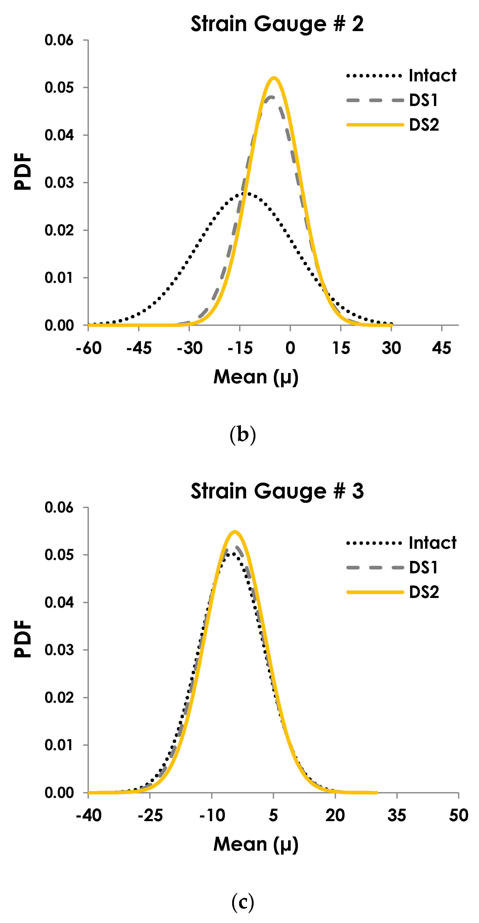
| Variation of µ | Variation of σ | |||
|---|---|---|---|---|
| Intact to DS1 | DS1 to DS2 | Intact to DS1 | DS1 to DS2 | |
| Strain Gauge 1 | −55% | −16% | −41% | −9% |
| Strain Gauge 2 | −57% | −14% | −42% | −8% |
| Strain Gauge 3 | −6% | −10% | −3% | −5% |
© 2019 by the authors. Licensee MDPI, Basel, Switzerland. This article is an open access article distributed under the terms and conditions of the Creative Commons Attribution (CC BY) license (http://creativecommons.org/licenses/by/4.0/).
Share and Cite
Bolandi, H.; Lajnef, N.; Jiao, P.; Barri, K.; Hasni, H.; Alavi, A.H. A Novel Data Reduction Approach for Structural Health Monitoring Systems. Sensors 2019, 19, 4823. https://doi.org/10.3390/s19224823
Bolandi H, Lajnef N, Jiao P, Barri K, Hasni H, Alavi AH. A Novel Data Reduction Approach for Structural Health Monitoring Systems. Sensors. 2019; 19(22):4823. https://doi.org/10.3390/s19224823
Chicago/Turabian StyleBolandi, Hamed, Nizar Lajnef, Pengcheng Jiao, Kaveh Barri, Hassene Hasni, and Amir H. Alavi. 2019. "A Novel Data Reduction Approach for Structural Health Monitoring Systems" Sensors 19, no. 22: 4823. https://doi.org/10.3390/s19224823
APA StyleBolandi, H., Lajnef, N., Jiao, P., Barri, K., Hasni, H., & Alavi, A. H. (2019). A Novel Data Reduction Approach for Structural Health Monitoring Systems. Sensors, 19(22), 4823. https://doi.org/10.3390/s19224823