1. Introduction
In 2000, the U.S. government turned off the selective availability of the Global Positioning System (GPS), making it more responsive to civil and commercial use. Since then, the industry of GNSS-based technologies (Global Navigation Satellite Systems, which includes other satellite constellations) has grown significantly. Surveyors, researchers, and most civilians use products developed from this technology. At present, GNSS receivers can be found in many devices, from precise measuring instruments to cellphones and cars. In the field of geodesy, GNSS has facilitated the implementation and quality control of high-precision and accurate networks. Before the advent of GNSS, establishing a geodetic network required a direct intervisibility between the points, as in triangulation and traverse surveys [
1]. Now, point co-ordinates can be defined by GNSS signals coming from orbital space, which only requires a good coverage of satellites during data collection. This has brought great flexibility in network design, and the achievable accuracy has also helped the densification of classical first-order geodetic networks [
2].
Most geodetic networks have been established using GNSS signals, which are available all over the Earth’s surface. They are defined by several materialized points with high precision and their co-ordinates serve as a basis in a wide variety of applications. Some examples are: support and basic control for surveying and mapping projects; implementation and maintenance of infrastructure works; monitoring of structural deformations; land cadastre and management; and monitoring of geodynamic events, such as earthquakes, landslides, and volcanoes. The study of Mt. Etna is a good example; two GNSS-based networks found a motion pattern of the active Nizzeti faults [
3]. In addition, a geodetic network design was applied to find optimal ground locations for interferometric synthetic aperture radar (InSAR) devices [
4].
To establish a geodetic network using GNSS, the receivers need to be placed at benchmarks and record satellite tracking data over a given period. Then, baseline vectors are determined between pairs of receivers, based on ranging and phase observations to the satellites. Once the vectors are computed, they become the new observations of the network and need to be adjusted to get the final point co-ordinates [
1].
Although most of the GNSS observation process does not require much direct human influence, the vectors may not be free of blunders. There are sources of error that may cause significant deviations (e.g., multipath signal propagation error, cycle slips, and ionospheric anomalies). The electromagnetic wave assumed to propagate along the line of sight between the satellite and the receiver might be reflected or scattered by obstructions before reaching the instrument [
5]. Other error sources are more mundane, such as mistakes in measuring the height of the antenna above the marker. Although random errors are inherent to observations, outliers should be detected, identified, and adapted for better determination of the co-ordinates [
6]. An outlier is better not to be used (or not used as it is) in an adjustment process because it has a high probability of being caused by a gross error [
7]. In geodesy, outliers are mostly produced by gross errors, and gross errors most often lead to outliers.
As outliers in observations affect the accuracy, those errors need to be identified or minimized [
8]. In standard geodetic adjustments, a least squares (LS) process is often applied, as it is the best linear unbiased estimator, assuming that no outliers and/or systematic errors are present in observations [
1,
9,
10]. If the data are contaminated, however, such an estimation will lead to biased parameters [
11].
Alternatively, the adjustment can be based on Robust Estimators (REs), which are less sensitive to outliers. If some observations contain blunders or even systematic errors, the REs will be insensitive to those non-random errors when estimating the parameters [
11]. REs have a wide range of applications; for example, in [
12], a robust parameter-estimation method for a mixture model working with the weights of samples is presented. Furthermore, applications of non-Gaussian distributions on multipass SAR Interferometry have been presented in [
13], and new methods for geodetic observations have been presented in [
14]. Therefore, they need to be investigated for a better understanding of their capabilities and limitations in geodetic networks.
The minimizing objective functions associated with REs are not linear and, therefore, iterative processes or smart techniques are required to solve them. One approach is to combine metaheuristic algorithms (MHs), to optimize the objective function. This strategy has been applied in several studies in geodesy, as it may lead to better results than classical methods [
15,
16,
17,
18,
19,
20,
21]. In MH research, the particle swarm optimization (PSO) [
22] has been widely applied, followed by the artificial bee colony [
23,
24,
25] and ant colony optimization methods [
26], more recently [
27]. Another solution is to apply a data-snooping procedure [
28,
29], a statistical test which takes place after the LS computation. However, studying statistical tests is not the purpose of this paper. Researchers have also applied MHs in others areas of geoscience, such as remote sensing [
30,
31].
For the adjustment of geodetic networks, MHs compute the unknown parameters (point co-ordinates) within a pre-defined search space and check them by evaluating the objective function for the chosen RE. The estimate is then used for the goodness-of-fitting evaluation. The process is repeated, following the exploration strategy adopted by the MH, until either an acceptable solution or the computational limit is reached [
20].
Applying MHs in geodetic networks adjustment has not been widely explored. Most studies have been limited to working with only one or two REs, often in simple cases. For example, they may not have considered the generation of multiple error scenarios [
18,
19,
21], or may have omitted the consideration of random errors [
20]. It is important to explore adjustment solutions where random errors can be simulated, getting as close to a real situation as possible. Still, several error scenarios need to be tested with a variety of REs to obtain a representative set and measure the reliability of the strategy.
Furthermore, an MH needs to present stable results when minimizing the RE functions and present good strategies to avoid local minima.
Therefore, this work has two main goals: First, developing better MHs by presenting the Independent Vortices Search (IVS) based on the Vortex Search method [
32], which brings advances to mitigate the limitations found in the original algorithm [
33]. We compare its performance with the original method, other modifications, and a competing algorithm.
The second goal is improving quality control in geodetic networks by combining smart and robust methods. By separating the results into three scenarios (with no outliers, small outliers, and large outliers), we classify the REs according to the demand and situation.
Then, the behaviors of several known REs when adjusting a geodetic network are tested: Least Trimmed Squares (LTS) [
34], Least Median of Squares (LMS) [
34], LTS-RC adding a constraint [
20], Sign-Constrained Robust Least Squares (SRLS) [
35], Least Trimmed Absolute deviations (LTA) [
36], and Iteratively Reweighted Least Squares (IRLS) [
37].
We generated observations from the official co-ordinates of a station and standard deviations from GNSS signal processing. Several error scenarios were simulated in the observations, which are tested by all REs, and the results are compared with the conventional LS. In addition, different median and trim positions in residual vectors of some REs are investigated. We analyzed the results by: (1) the identification outliers, analyzing the residuals vector, and (2) by the estimated parameters, comparing them with the official co-ordinates of the network.
Additionally, for problems based on the Gauss–Markov model, we present a new proposal for the search space definition when using MHs. Furthermore, a comprehensive analysis of the results achieved with different trim and median position in some REs is given, showing which equation is best in each situation.
This paper is organized into six sections: In
Section 2, we present a theoretical overview of the LS and RE methods applied in the experiments.
Section 3 presents the first contribution of the study, showing the Independent Vortices Search algorithm. In
Section 4, we present details of the experimental setup, how we analyzed the quality of the solutions, and the implementation of the REs and IVS.
Section 5 presents the second contribution of this work, discussing the results obtained with adjustments to the GNSS network. We compare the results of the trim and median position of some REs and the outcomes, as well as discussing the various error scenarios.
Section 6 brings the final considerations about the research and suggests issues to explore in future research.
3. Independent Vortices Search
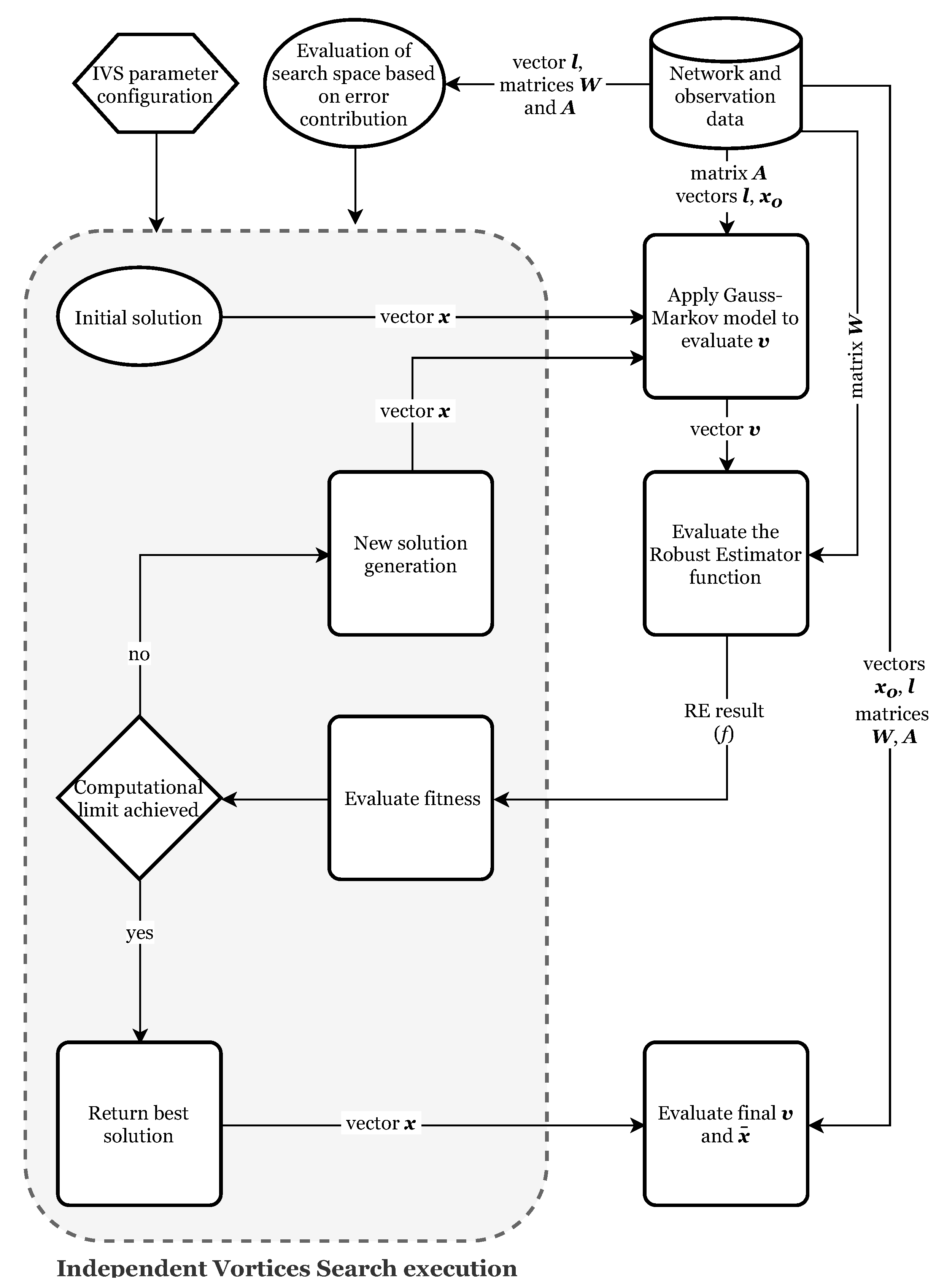
All of the REs (except for IRLS) require a numerical optimization method. The MH has to explore values for the parameters which generate the residuals from the Gauss–Markov model. The objective function of the RE is then evaluated and used for the computation of the solution fitness. Then, the MH generates new candidate solutions, continuing the process until it reaches a pre-defined limit [
20].
For the numerical optimization, we developed the Independent Vortices Search (IVS), based on the Vortex Search algorithm (VS) [
32] and its modification, the Modified Vortex Search algorithm (MVS) [
33]. While VS works with one vortex, MVS can explore many vortices at once, exchanging information. We will present more details below.
3.1. Vortex Search Algorithm
The Vortex Search algorithm (VS) is a single solution MH for numerical function optimization. It generates new candidates around the current best result, moving along the search space when achieving a better solution. The radius defines the limit for generating new candidate solutions and decreases over cycles [
32].
VS and MVS define the initial radius (radii) of the center (centers) by using Equation (
19), covering the whole search space. The algorithms obtain their first solution by applying Equation (
20), causing the search to begin at the center of the space:
where
is the initial radius of the
jth parameter,
and
are the respective minimum and maximum limits of
jth parameter, and
is the center of the vortex and the initial solution for the parameter
j.
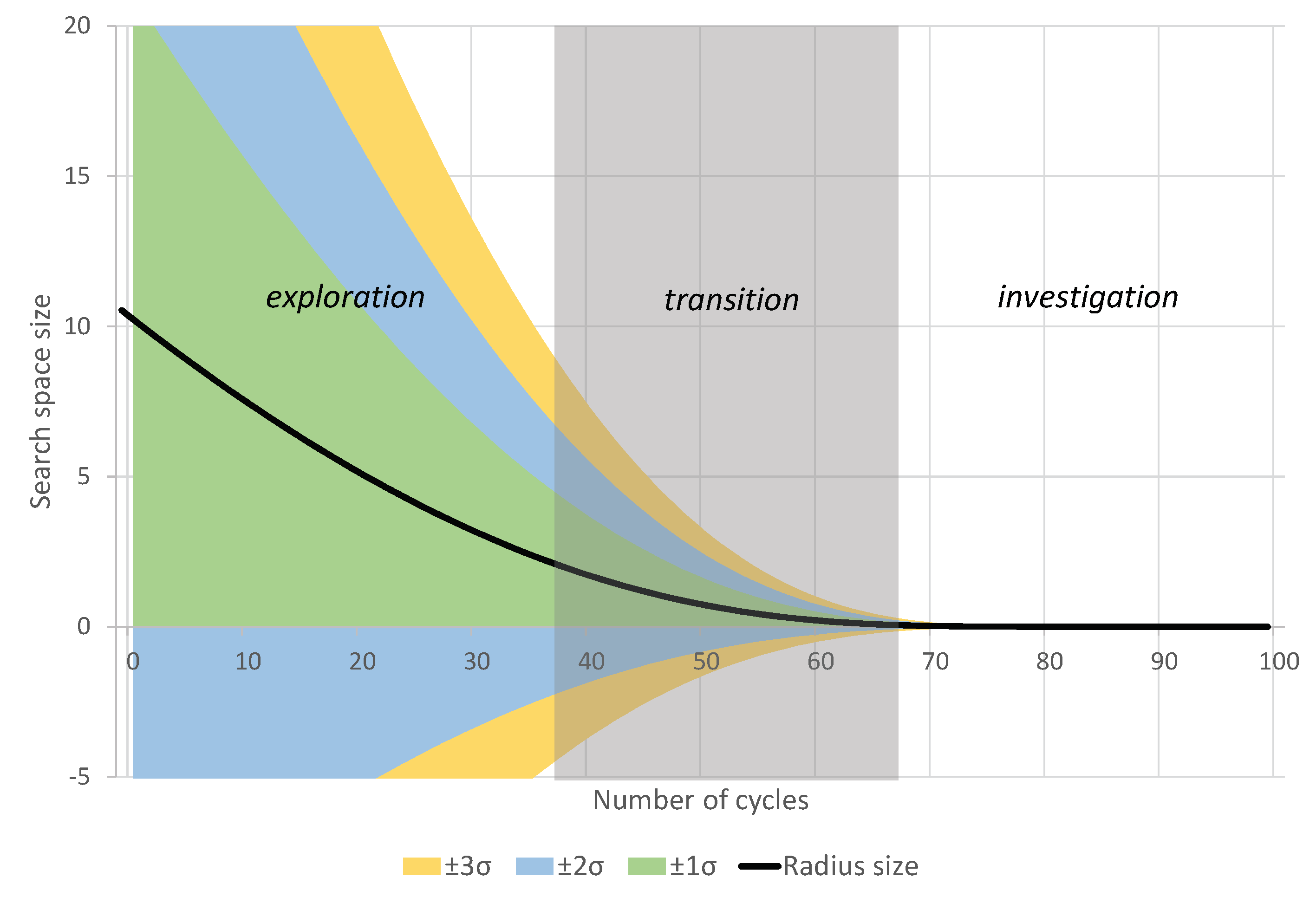
In each cycle, the radius decreases to limit the generation space for new candidate solutions. In the later cycles, the VS produces a fine adjustment as the current candidates get closer to the best solution. The radius decrease is obtained by Equation (
21), and provides satisfactory control of the exploration and investigation [
32]:
where
is the radius size in cycle
c,
R is a constant (set at
) that controls the resolution of the algorithm’s search, and
is the incomplete inverse gamma function, given by Equation (
22):
where
is a parameter that defines the shape for each cycle, as defined by Equation (
23):
The equation of the shape parameter uses the cycle count c and the maximum number of iterations .
The vector of candidate solutions
is randomly generated at the center
using the Multivariate Normal Distribution (MND) with the standard deviation vector of
.
Figure 1 shows an example of the radius convergence by applying Equation (
21) and the candidate generation limits by the MND.
The algorithm checks that the candidate values are within the search space by applying Equation (
24), where
is a random real value between [0, 1]:
For each candidate solution, a fitness function tests the result: If a candidate produces a better outcome than the current one, VS moves the center () to the new solution and discards the remaining candidates. Otherwise, the algorithm keeps the best obtained result and produces new solutions.
Both VS and MVS use all the above equations. However, by using several vortices, MVS adjusts the positions of its centers to each cycle, based on the vortex, with a better result. This separates positioning the center
for the generation of new solutions, and the best solution
of a vortex
l. For this, MVS applies Equation (
25):
where
is the new position of the center
l,
is the best solution of the center
l, and
is the result of the vortex with the best solution. At each cycle, all centers (except for
) gain new positions using the above equation [
32].
As has been shown, VS has no crossover nor mutations between candidate solutions, unlike Genetic Algorithms (GAs) and the Artificial Bee Colony (ABC) method. At each cycle, it saves the best solution—either the current best or a new one—for the next cycle, discarding the remaining ones. This way, VS has no need to use individual selection strategies, a mutation rate, or other strategies present in other MHs. This helps to keep the configuration simple, reducing human interference in searching for a solution to a problem.
Another interesting characteristic of VS is the transition between global and local search. In many MHs, exploration and investigation occur from the beginning to the end of the execution. This makes it possible to find a good enough solution, even in the first few cycles. This way, they can interrupt the execution if so desired. Otherwise, the global search continues through to the last iterations, attempting to reduce the risk of local minima. In VS, the radius size is reduced over the cycles using an inverse incomplete gamma function (Equation (
22)) and considering the ratio of cycles performed (Equation (
21)). Thus, exploration and investigation occur gradually, and so are not present throughout the entire execution, yet still providing an adequate balance. The advantage of this strategy is the fine-tuning of the best solution found in the last cycles.
However, by analyzing the VS strategy, we can conclude that the transition between exploration and investigation has two drawbacks. First, it has the local minimum risk: There is no possibility of achieving the global solution in an execution if it limits the radius to a local minimum area. The radius of the vortex becomes small and the candidates get stuck in a local search limitation. The second inconvenience is identifying the dispensability of the processing during the execution. When defining a limit of execution for example, by the number of cycles, it executes them in its totality because only in the later cycles does VS carry out the investigation stage.
MVS tries to minimize the local problem by adding several vortices to VS. However, applying Equation (
25) does not mean the vortex with the so-far best solution will bring the other centers closer to a global minimum.
With these characteristics in mind, we based the proposed IVS method on maintaining solution fine-tuning while trying to circumvent the local minimum problem, all without increasing the computational cost.
3.2. Characteristics of the IVS
The IVS starts from the MVS, aiming to make it simpler and more efficient. We propose three strategies through which IVS differs from MVS.
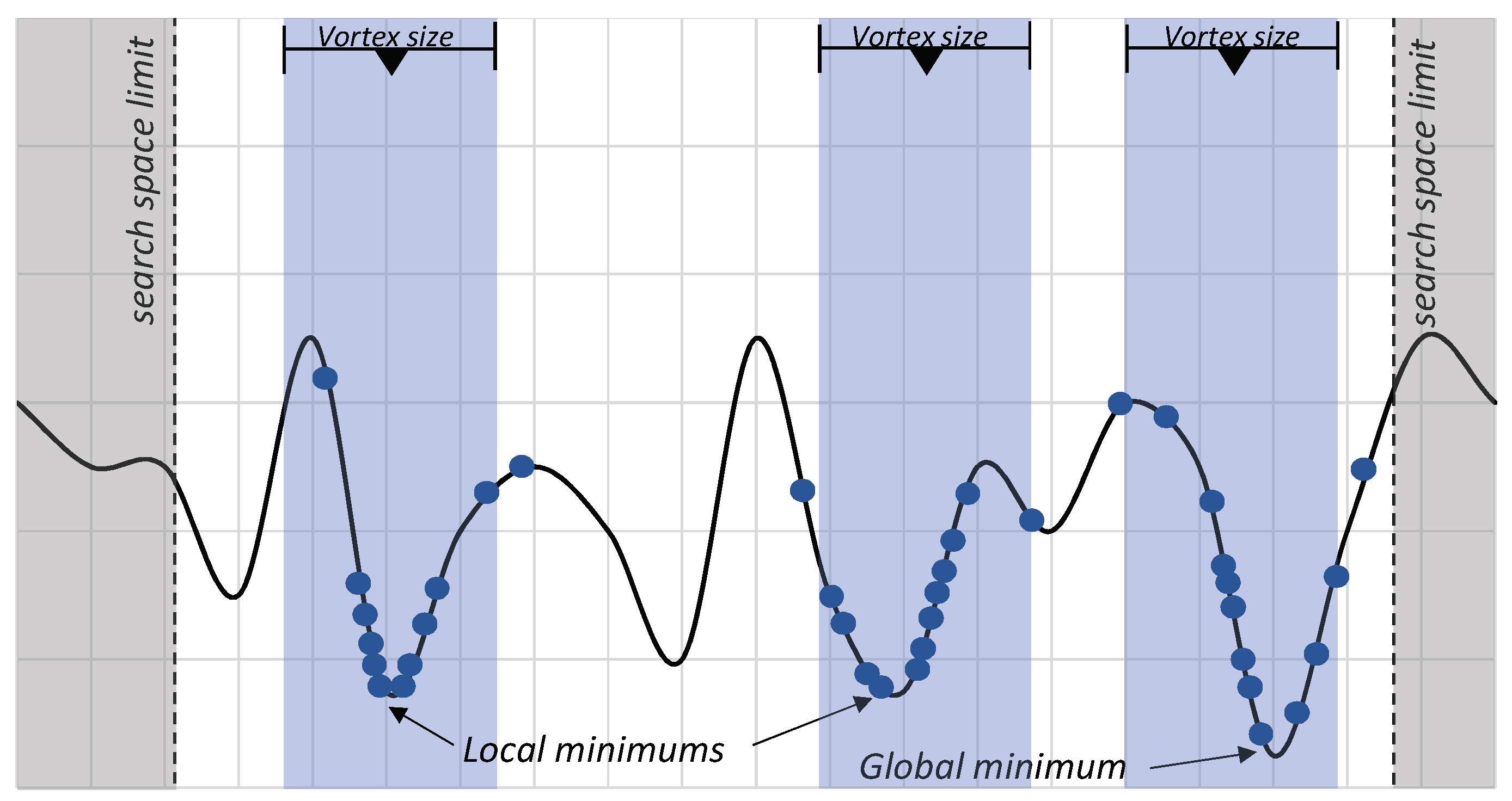
The first major difference is the complete elimination of Equation (
25), which changes the vortex center positions, based on the vortex with the best result. By doing so, each vortex can proceed toward a minimum, whether local or global. This is intended to minimize the local solutions, as we can add more vortices to explore solutions independently.
Figure 2 presents a hypothetical situation in which the vortices follow their paths towards the minima.
The second feature of IVS is the replacement of Equation (
20) for each additional vortex. The first vortex has an initial solution defined by applying Equation (
20), whereas the remaining, by Equation (
26), are randomly distributed in the search space:
where
is the initial solution for the
jth parameter of the vortex
l, with
,
, and
are the respective minimum and maximum limits of the
jth parameter
is a random real value in the interval [0, 1].
The third modification considers maintaining the amount of candidates per vortex when
(where
L is the total number of vortices). In the MVS proposal [
33], the experiments presented five centers and divided the number of candidates between them. IVS, however, fixes the quantity of candidates for each vortex. To compensate for the computational increase, IVS decreases the number of cycles performed to keep the total Fitness Evaluations (FEs) the same.
It is still possible to verify that the first two strategies have the possibility of a higher diversity of the candidates generated. By removing Equation (
25), each vortex is allowed to go ahead with its search, not dragging them close to a vortex, with better overall results at the moment. The second strategy (Equation (
26)) allows for greater diversification while generating the first results. This is because the MND, which uses the center of the vortex as the mean for candidate generation, generates more solutions near the center. With the centers of vortices more widely distributed, IVS should not concentrate candidates in only a part of the search space.
3.3. A New Search Space Definition
For the definition of the search space in the adjustment of geodetic networks, we defined the limits of each parameter
j by
and
. By using the parameter vector
obtained from conventional LS computation, we set the exploration area according to Equation (
27):
where
is the greatest absolute residual from the LS solution,
is the greatest absorption fraction of an error and 1.15 indicates a 15% safety margin. Additionally,
is defined by Equation (
28) [
44]:
where
is the covariance matrix of adjusted residuals from the LS solution.
Equation (
27) presents a novel method to define the search space. It can be applied to any problem susceptible to outliers that use the Gauss–Markov model to generate residuals and MH to explore the solution. It is not limited to geodetic networks and can be used along with REs or other techniques—for example, in hyperspectral image data [
45,
46] or 3D Point Clouds [
47]. Applying this strategy to 900 scenarios, it did not omit any solution in the IVS exploration limit.
5. Results and Discussion
For better comprehension, this section is divided into three subsections:
Section 5.1 presents the optimization with IVS and comparison with the performances of other MHs.
Section 5.2 shows the estimated impact of the trim limit and median position in some REs, when applied to the geodetic network adjustment.
Section 5.3 presents the results for the network adjustments, applying IVS and testing all the REs (including the trim limit and median position variations) in 900 error scenarios. The adjustments were organized in three topics: no outlier case, small magnitude outliers, and large magnitude outliers.
5.1. Performance and Discussion of IVS
We conducted several tests to compare the solutions obtained with IVS to solutions obtained by other MHs. For a better analysis, we generated four scenarios of errors in a GNSS network. Each scenario contained three simultaneous outliers, ranging from , in 39 observations (about 7.8% contamination). Using the LMS estimator, the MHs executed the scenarios twenty-five times. This allowed for analyzing the stability and quality of the results. More details of the network can be found in the next section.
Besides the MHs already presented, we also tested the Hybrid Vortex Search algorithm (HVS). The HVS works with the combination of ABC and VS, trying to take advantage of the best characteristics of each strategy. The reader can find more details in [
49]. Thus, the algorithms tested were:
The configurations of the MHs obeyed the following parameters: 5,000,000 FE as processing limit, 50 candidates per center for vortex algorithms, and 50 bees in ABC (25 food sources). In addition, we tested the MVS and IVS with five vortices, as presented in [
33], and 40 vortices. Preliminary tests showed better results from 20 to 60 vortices, so we adopted an intermediate value of 40.
It is important to note that cycle counting was not used as a configuration parameter or as a limit for the MH executions. For more objective comparisons between MHs, we should not use the cycle count as a stopping criterion. As each MH has different strategies in its execution, it can use a different quantity of FE in each cycle. Using a fixed number of cycles as a parameter to limit the execution can cause a large variation in the total amount of FE for each MH. This would favor MHs that make more FE per cycle, since they have more opportunities to test their solutions [
50]. We adapted the algorithms to use the number of FE as the limit for suspension. This allowed for a more adequate performance comparison. To better situate the reader, executing 5,000,000 FE was equal to 100,000 cycles in ABC with 50 bees (25 food sources); 100,000 cycles in VS with 50 candidates; and 20,000 cycles in IVS with five vortices and 50 candidates per center.
The MVS experiments performed in [
33] divided the quantity of candidates by the number of vortices. Thus, in executions with 50 candidates and five vortices, MVS generated only 10 candidates per vortex every cycle. As this work uses the number of FE as the execution limit of the MHs, each vortex generated a number of candidates established by the number of candidates parameter. For a run with 50 candidates and five vortices, the algorithm generated 50 candidates per vortex each cycle. This characteristic is standard in IVS.
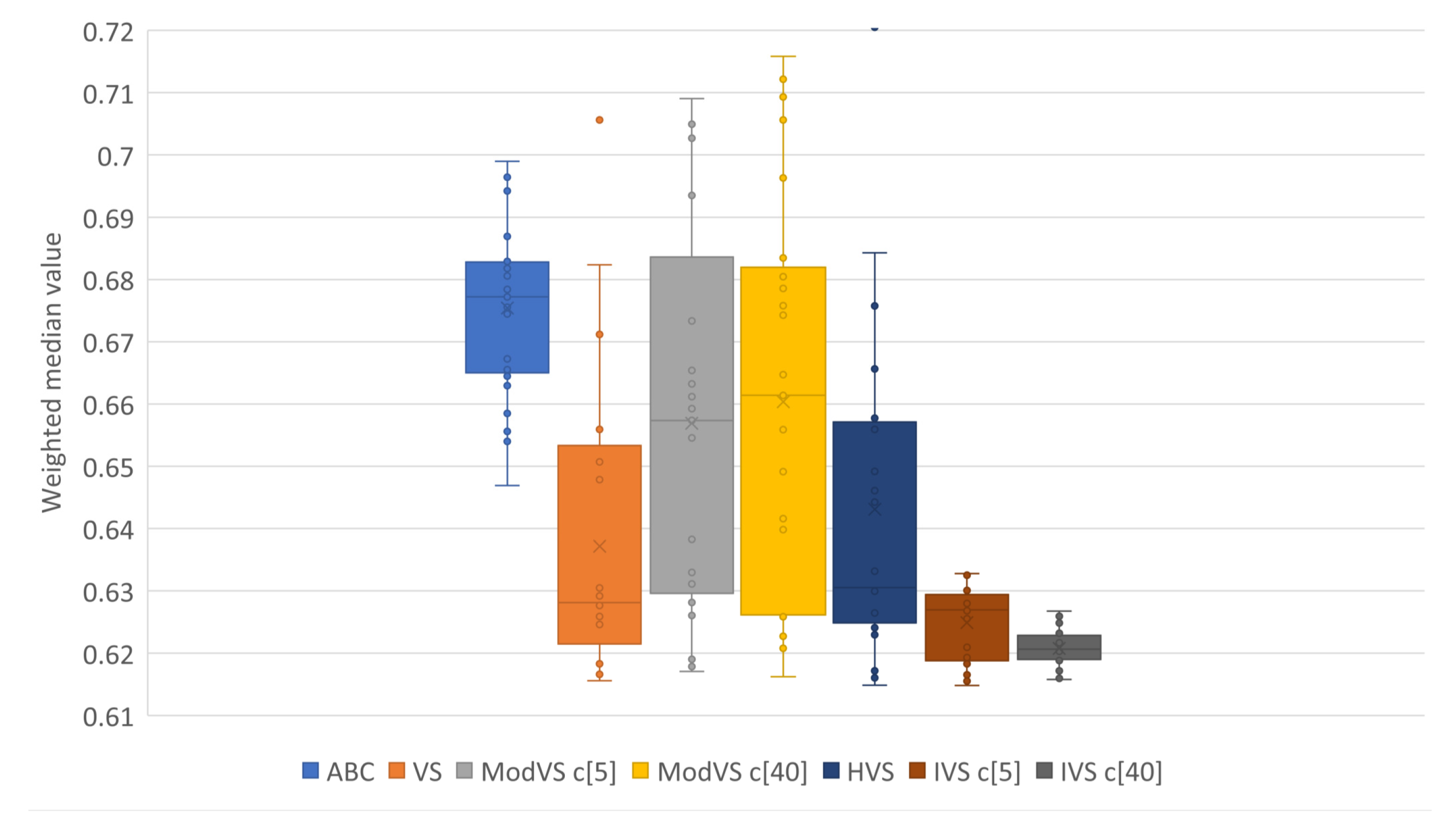
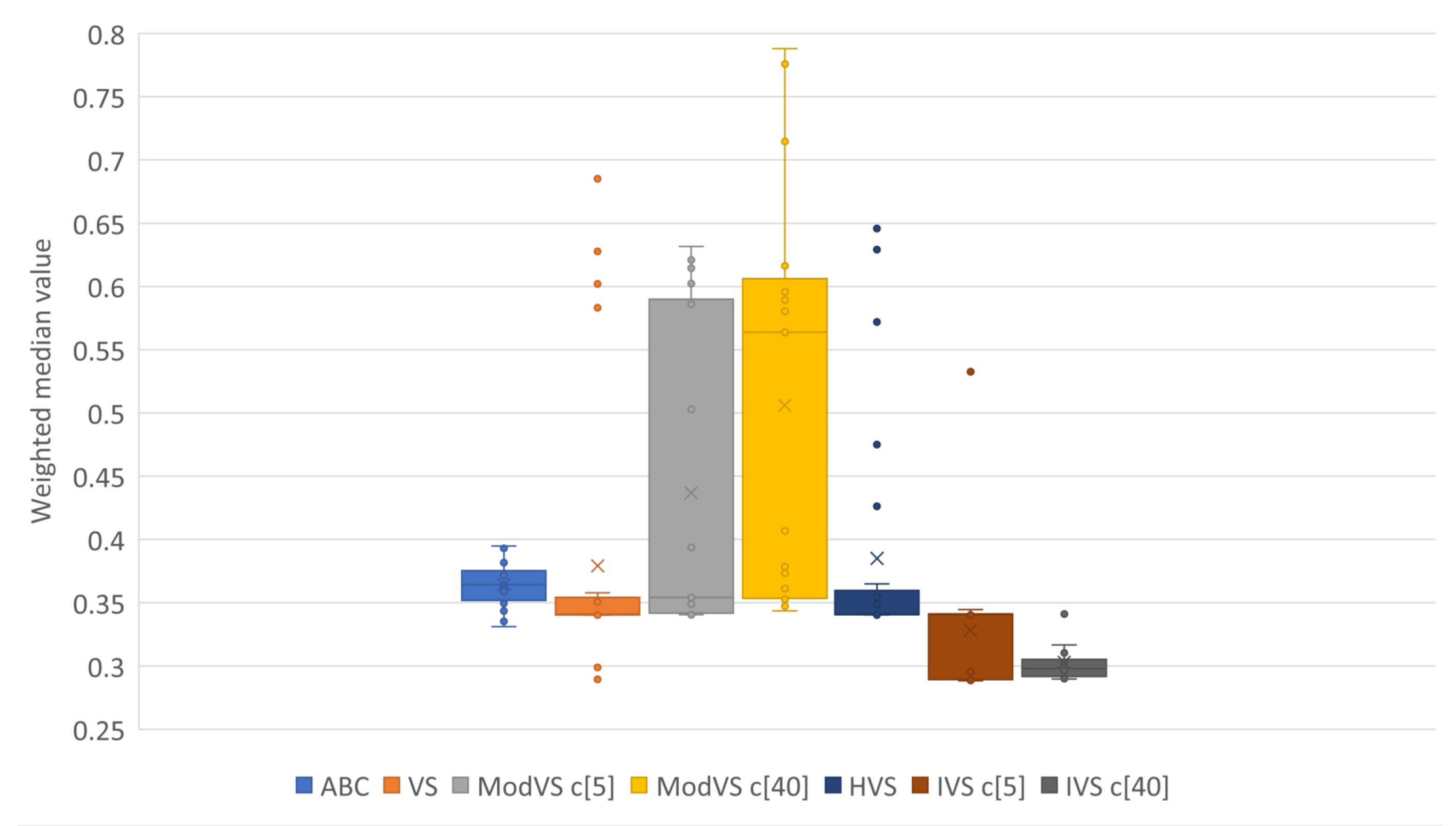
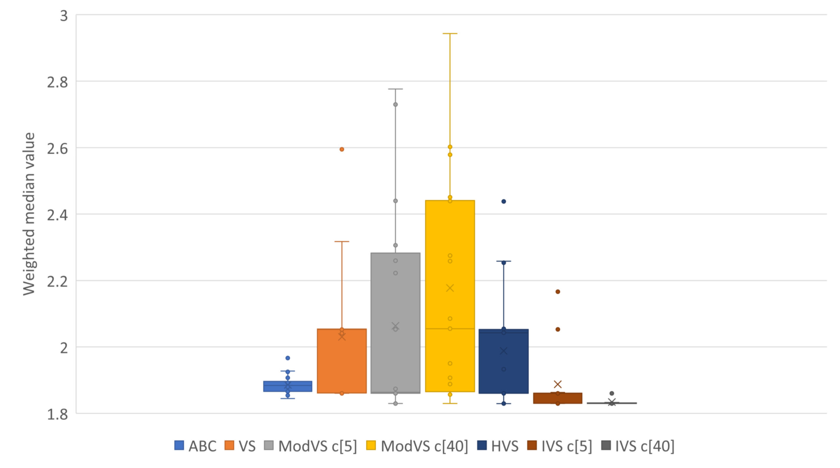
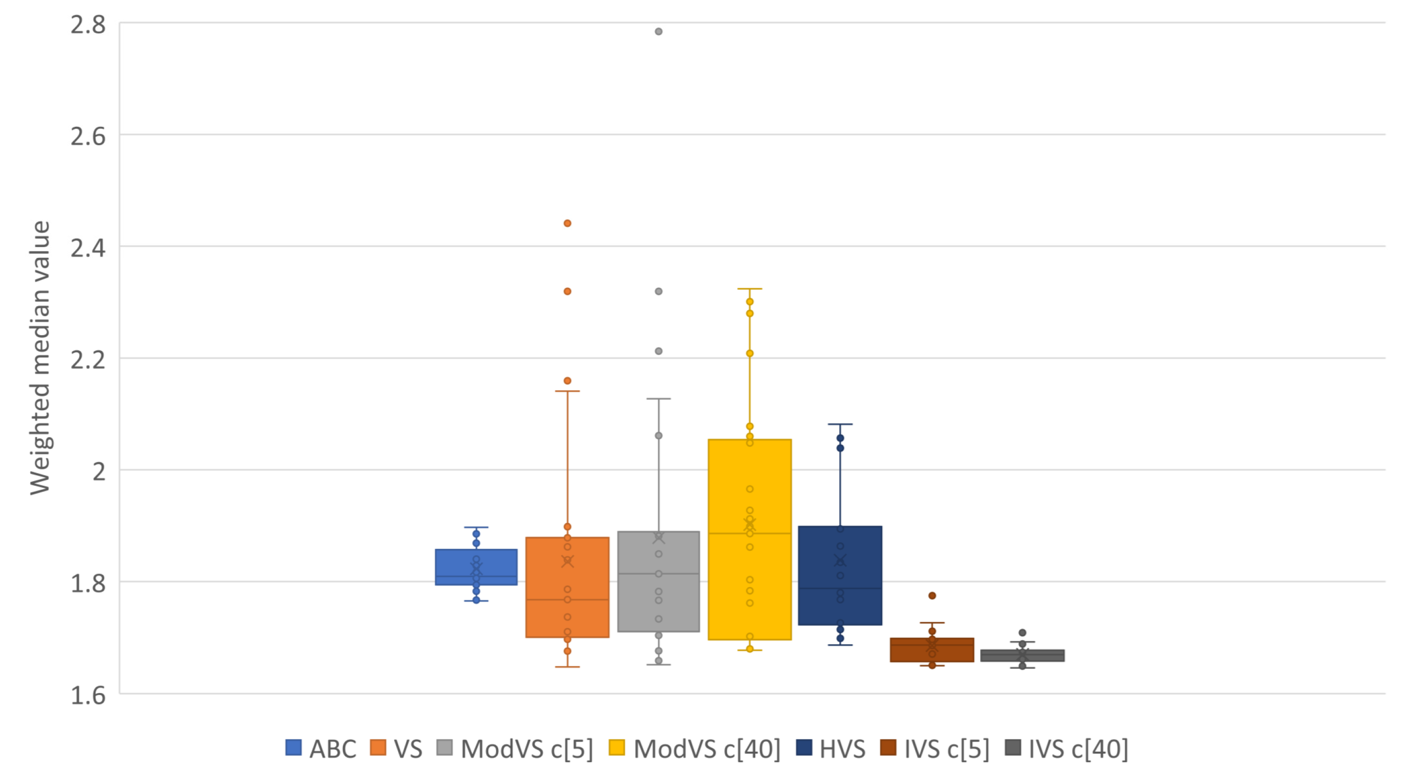
For better representation of results, we present them in box plots. Each point represents the result of one run. The number after “c” in brackets (e.g., “c[5]” and “c[40]”) is the amount of vortices, where applicable.
Figure 5,
Figure 6,
Figure 7 and
Figure 8 show the results for Scenarios 01, 02, 03, and 04, respectively.
By analyzing the charts, we see that IVS performed better than other MHs. The configuration with 40 vortices overcame the alternative with five vortices, although both options showed good results. IVS achieved the lowest minimum and presented little variation. The HVS strategy did not improve much on the solutions, as they were similiar to those found by the original VS. ABC showed lower variation in the results when compared to the already known MHs. This shows a certain stability in the solutions, surpassed only by IVS.
It is also possible to note the horizontal alignments of points (solutions) in the charts. This was common to several MHs and identifies the local minimums in which the MHs got stuck in, on some runs. In
Figure 7, it is possible to notice an alignment between the values
and
for MVS and HVS. The same diagram shows another alignment between
and
for all MHs, which coincided with the bottom of the boxes for the VS, MVS, and HVS solutions.
The MH proposed in this work overcame all other tested MH in both the mean and variation of the solution. It needed no extra computation, producing the first scientific contribution of this work. We applied the IVS configuration with 40 vortices in the following experiments to optimize the RE functions.
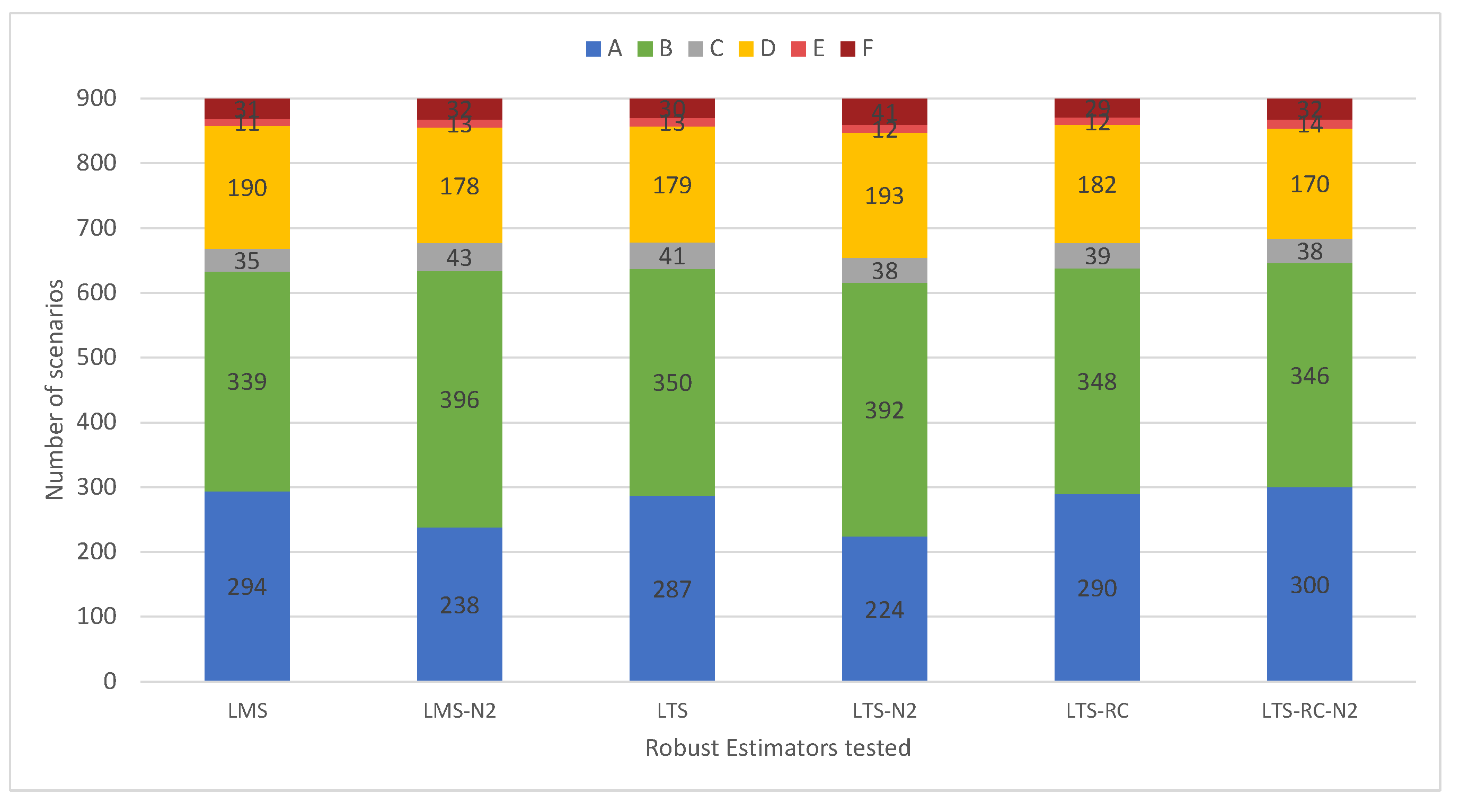
5.2. Comparing LTS/LTS-RC Trim Limit and LMS Median Position
We performed tests with the two values for the limits of LTS and LTS-RC and for the median position of LMS. The lower limit, , will be shown as and the upper limit, , as .
Figure 9 shows that the adjustments with the limit of
had worse results in the classification for LMS and LTS. Classifications of type “A” were reduced by adopting the expected threshold, as compared to more robust, increased “B” classifications. For these estimators, the lower limit maintained outliers identification, but pointed out more false positives. The results for the LTS-RC present a slight improvement to the limit of
.
Comparing the results of LTS and LTS-RC, we notice that the results presented almost the same classifications, whereas the variations with presented a significant difference. This is because the larger limit () removed fewer residuals, hardly breaking the redundancy. Furthermore, since the network had several observations among its three-dimensional points (although not repeated), it was hard for any parameter to remain without at least two residuals (not breaking redundancy). Using the limit of , the classic LTS more easily broke the redundancy in the residuals trim, whereas the LTS-RC achieved more satisfactory results, retaining the redundancy of the network.
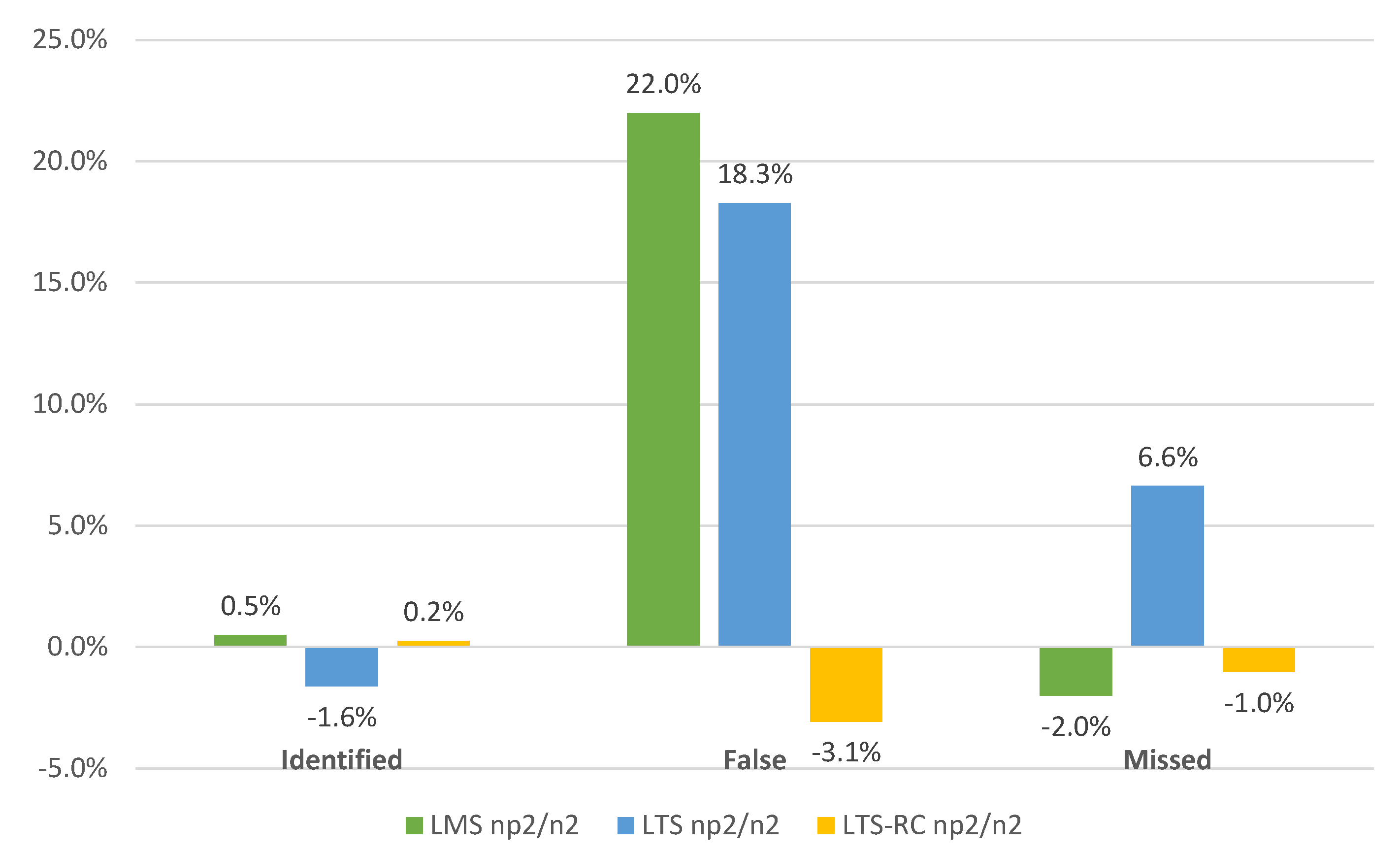
Figure 10 confirms a gain of false positives with the limit of
for LMS and LTS, and stability with a slight improvement for LTS-RC. There were no significant differences in outlier identification for the different limits, while, for undetected errors, only the LTS showed a 6.6% worsening.
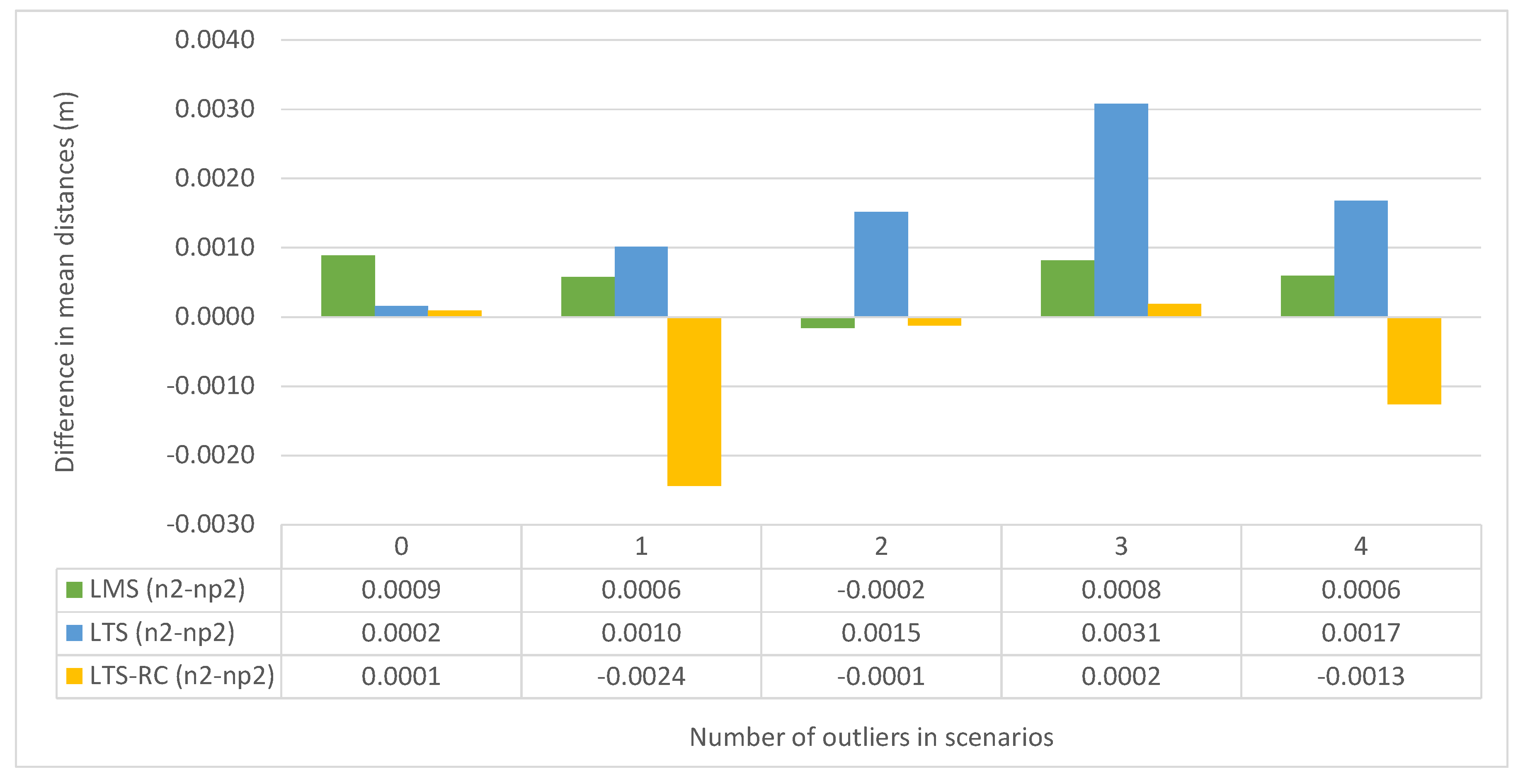
We also compared the distance of the co-ordinates from their true values.
Figure 11 displays the mean distance difference of the co-ordinates in each scenario package, between the limits
and
, for each RE. The mean differences were negligible in most situations, being below 1 mm with either
or
. LTS produced inferior results with
, whereas the LTS-RC reduced the variation in two cases, with one and four simultaneous outliers.
The redundancy constraint has proven to be interesting for any problems where the number of observations per parameter is more limited and/or the trim limit is smaller. To the best of our knowledge, this is the first time the h value has been analyzed for a geodetic application. As the measurements of these networks do not contain data related to all the parameters, the redundancy constraint also played an important role. Besides this specific treatment, the h value can be considered in any studies that wish to apply LMS, LTS, or LTS-RC.
5.3. Results in Network Adjustments
For better analysis of the behavior of each RE, we divided the results into three topics: the no outlier case (Package 01); scenarios with small outliers (Packages 02, 04, 06, and 08); and scenarios with outliers of great magnitude (Packages 03, 05, 07, and 09).
5.3.1. No Outlier Case
For scenario package 01, the results confirmed the statements in the literature. The conventional Least Squares method (LS) was the best linear unbiased estimator when the observations were free of outliers.
The solution classifications by detecting outliers in the residuals are shown in
Figure 12. LS had excellent performance, with no false positives, getting an “A” classification in all scenarios. Most REs showed similar results, with about half of the classifications as “A”.
This means that all REs presented false positives in some scenarios.
Figure 13 shows the false positive counts for each estimator. Most estimators achieved similar results, with almost one false positive per scenario.
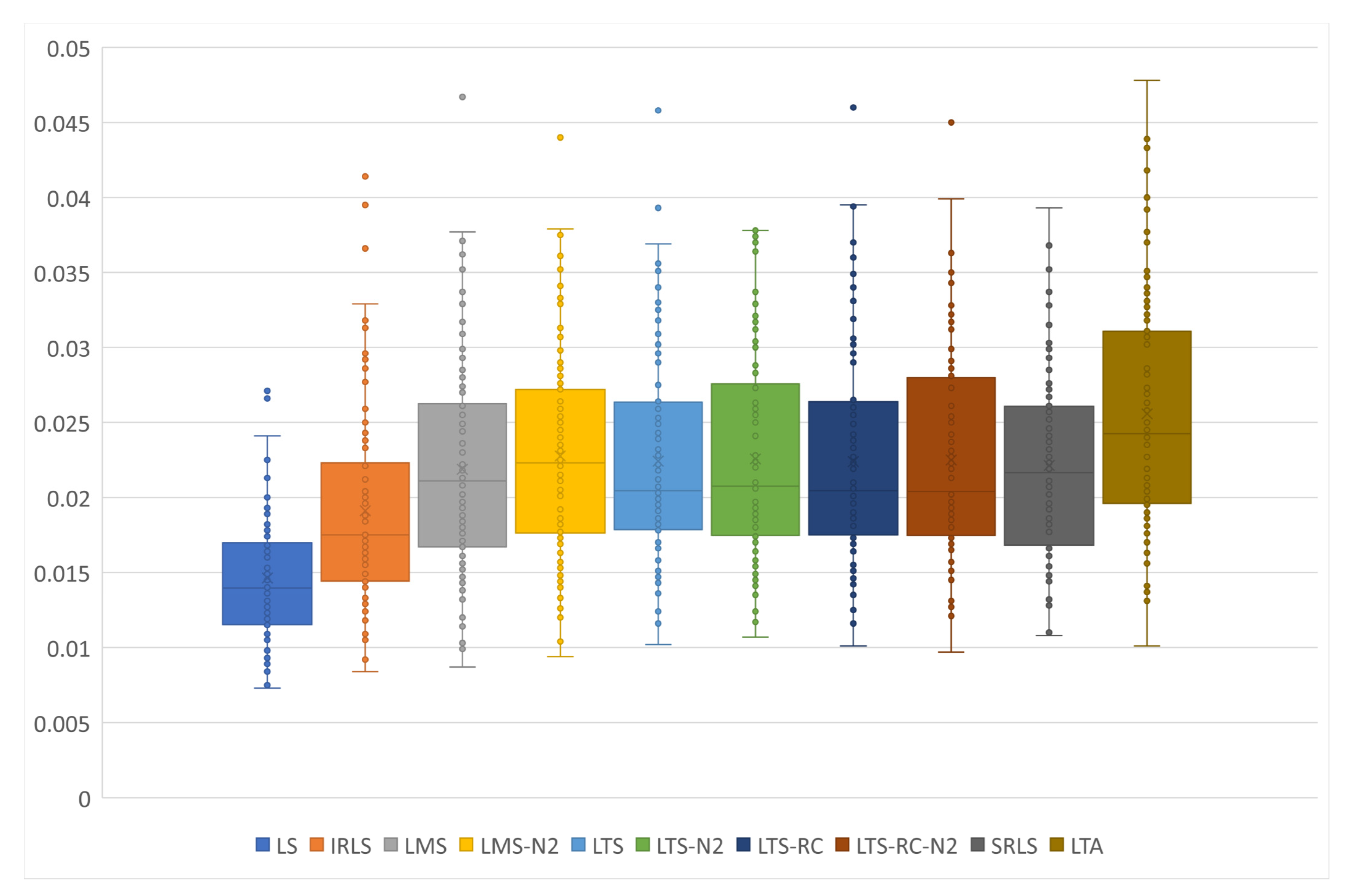
To check the solutions of each estimator, we elaborated the box-plot chart shown in
Figure 14. The LS exceeded all other estimators, showing a lower variance and a lower variation between the scenarios. As expected, the LS estimation was superior to any other RE, when tested in the conditions of no outliers. In addition, LS required no MH to estimate the parameters and presented low computational cost, when compared with estimators that need MHs. It is important to point out that the points will not reach zero, due to the random errors present in all observation vectors.
Both for outlier identification and co-ordinate estimation, LS proved to be the best method for scenarios with no outliers. The high number of false positives in the other estimators solutions led to discarding good observations and greater deviations in the estimation.
5.3.2. Small Magnitude Outliers
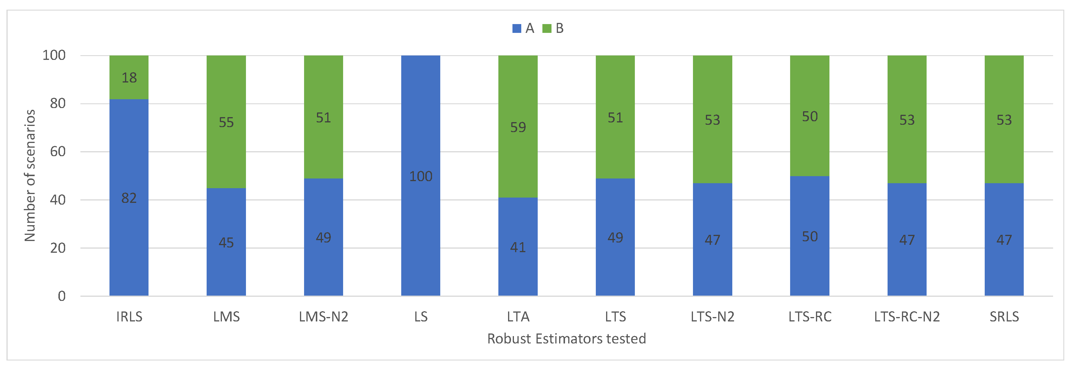
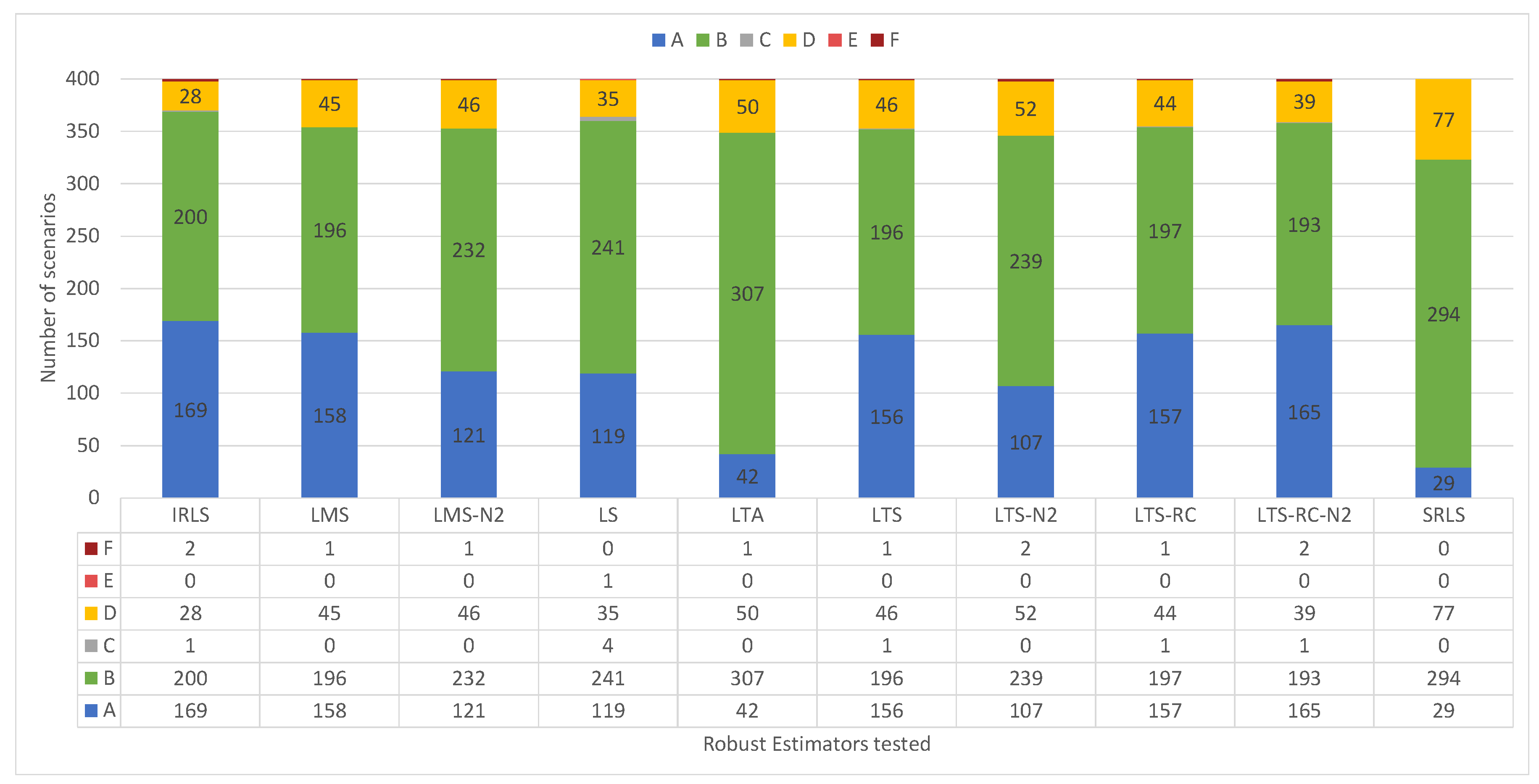
Starting with the outlier detection,
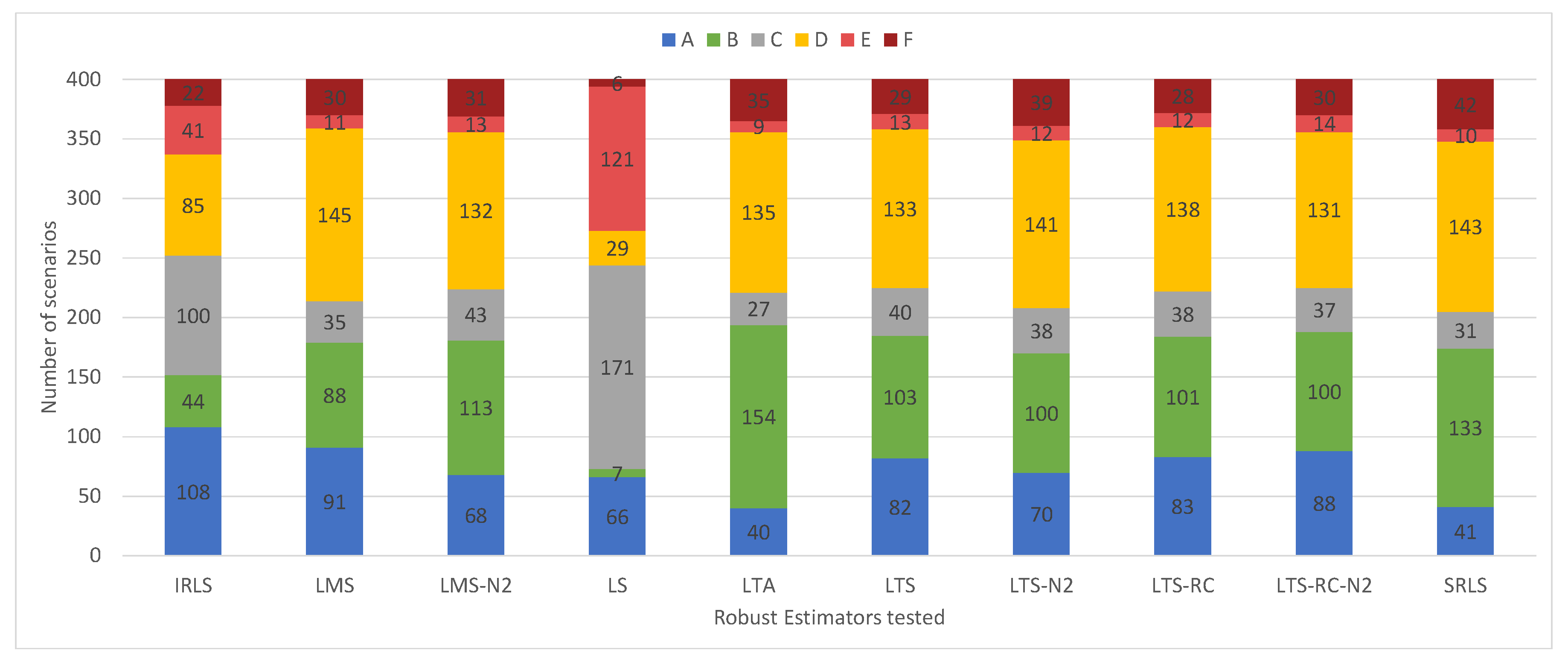
Figure 15 gives the solution classifications for each RE in the 400 scenarios. LS presents its results concentrated in the ‘no false positives’ classifications (“A”, “C” and “E”). This shows a resistance for pointing out false positives in the residuals vector by LS solutions. The IRLS got the highest number of solutions classified as “A”, overcoming the other estimators. By checking the results for classifications that identified all outliers (“A” + “B”), the LMS, LTS, and LTS-RC-N2 had the best identification ability.
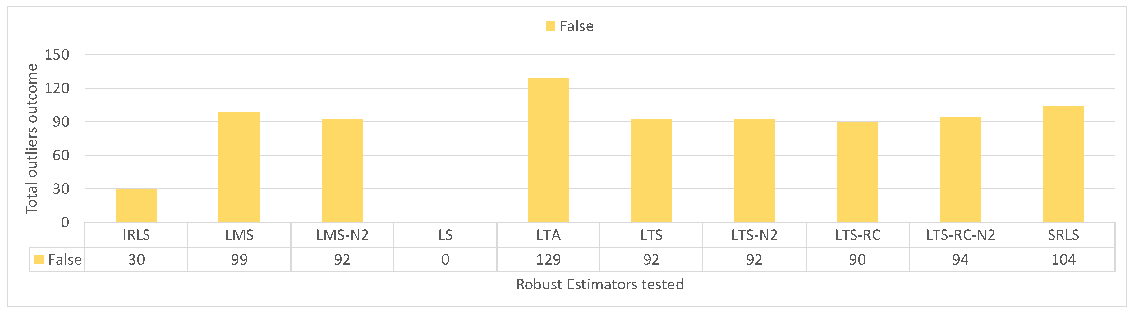
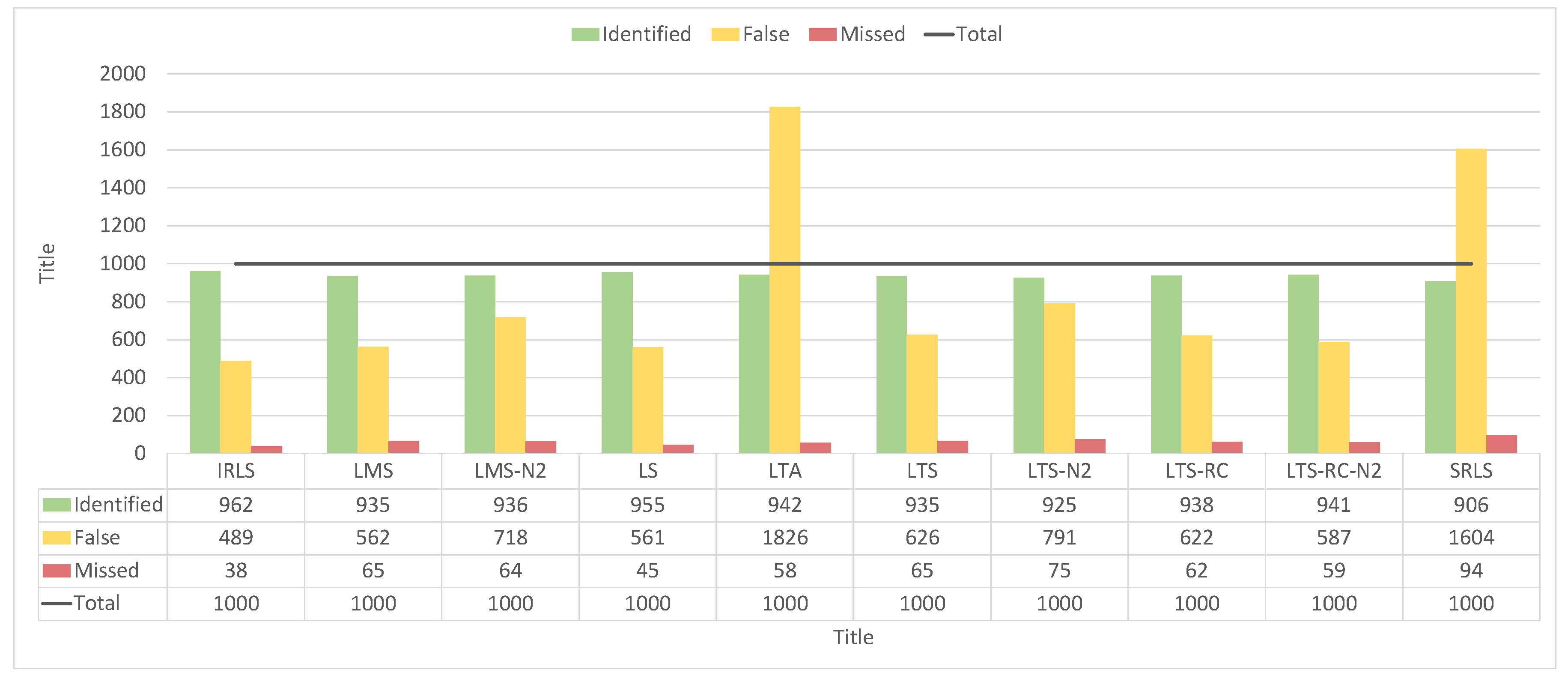
Although the LTA presented many classifications of type “B”, this estimator had the lowest number of solutions classified as type “A”, similar to SRLS. In
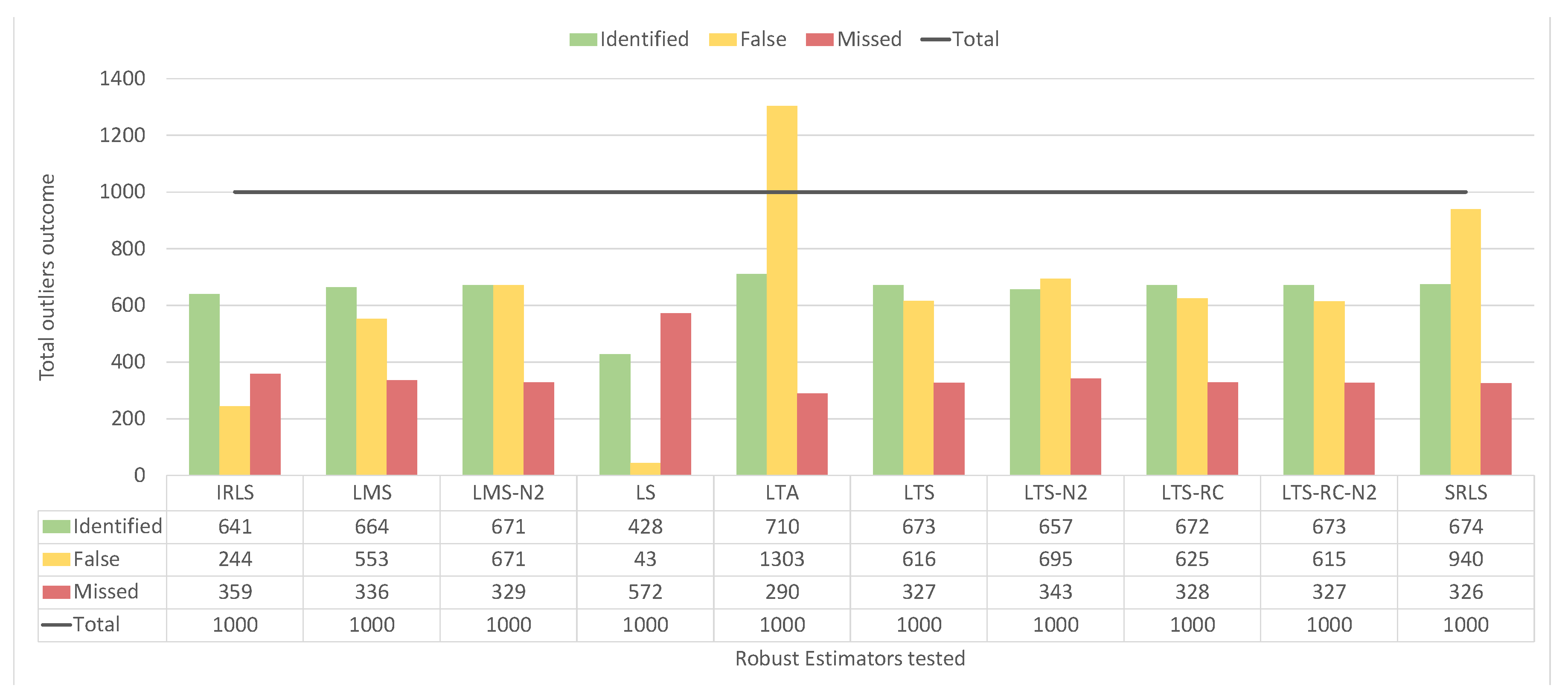
Figure 16, we see that LTA presented 1303 false positives in the residuals vector, over the 400 scenarios. It also confirms LS as the estimator with the least amount of false positives (43). In contrast, LS missed most of the blunders, not detecting 572 out of 1000 inserted outliers. Among the REs where IVS was applied, the LMS identified a good part of the outliers without an exaggerated quantity of false positives, missing less than IRLS and LS.
Analyzing the estimator solutions for parameter estimation,
Table 2 shows the mean distance of solutions from the official co-ordinates. It also adds the LS result without outliers, to compare the influence of the random errors.
LS presented the smallest deviations, being the best estimate of the parameters in the case of adopting the solution, without eliminating contaminated observations and making new adjustments. Even in scenarios with four outliers, the LS showed a better result than the REs, although the difference became smaller. The IRLS presented low variation in the solutions, even with an increase of blunders. Whereas most RE presented similar solutions, LTA, in contrast, had the worst estimates.
For an application where outliers should be identified, the LS method is not the best. In these cases, according to the results of the experiments, it is recommended to work with IRLS, or, for a better identification with a higher cost in false positives, LMS, LTS, and LTS-RC-N2 obtained more satisfying results.
By analyzing the estimates, LS presented a more solid estimate, even with the lowest detection of blunders. This shows that the outliers which were not detected by LS did not exert great distortion in the estimation. For both scenarios without outliers or schemes that present blunders of small magnitude, LS remains as the best estimator for the parameters. The good redundancy of the network probably contributed to this result. In networks with poorer geometry, the LS will not be as robust to small outliers.
5.3.3. Large Magnitude Outliers
In contrast to the experiments with small outliers, all REs showed greater ease in detecting larger outliers. Most the results were classified as “A’’ or “B’’, and rarely as “E’’ or “F’’ (see the classifications of the solutions in
Figure 17). In this case, LS presented solutions with false positives, “B’’ and “D’’ types, resembling the other tested estimators.
For classifications “A’’and “B’’ (i.e., all outliers were identified), the estimators presented similar results, around 90%.
By counting the detected false positives and undetected outliers, all estimators pointed out most of the blunders, as can we see from
Figure 18. For 1000 outliers, the values ranged from 906–962 for detection. As the detection of outliers is almost optimal, it remains to compare the amount of false positives, where IRLS, LS, LMS, and LTS-RC-N2 had the lowest false positive values, ranging from 489–587.
Table 3 presents the mean distance of solutions from the original co-ordinates. LS presented an unsatisfactory estimate for large outliers. The solution deteriorated, even with only one outlier of great magnitude. As we added more blunders to the scenarios, LS became one of the worst solutions for direct parameter estimation. LTA and SRLS also showed bad estimates, whereas most estimators presented similar, more satisfactory results, proving greater insensitivity to the outliers.
In general, for outlier identification, the LS, IRLS, LMS, or LTS-RC-N2 methods had better detection. Regarding the computational cost of these solutions, LS is the best choice because it has its own iterative method.
However, for the final estimate of the co-ordinates, the REs presented more satisfactory estimates. This shows the sensitivity of LS to outliers of great magnitude and the strength of robust methods.
Table 4 presents the best estimator, concerning the application and scenario of errors.
6. Conclusions and Future Works
Geodetic networks are the basis for mapping, geoinformation, land cadastre, and other location-based services. They play an important role in society in infrastructural works that depend on accurate control points. This work tested the strategy of using Robust Estimators (REs) in geodetic network adjustment and for detection of outliers.
Several REs were tested. A metaheuristic optimization was conducted for the LTS, LTS-RC, LMS, SRLS, and LTA estimators, whereas, for the IRLS, an iterative process was handled.
The two main contributions of the research were successfully demonstrated: (1) the Independent Vortices Search (IVS) overcame the VS, MVS, HVS, and ABC in all aspects; (2) we performed a deep investigation of several REs, separating the analysis scenarios into no outliers, small outliers, and outliers of great magnitude. This led to the classifications in
Table 4, something not explored in the literature before.
In addition, other minor contributions were also presented. One of them was the search space proposed for applying IVS using Equation (
27), which is valid not only for geodetic networks, but for any problem based on the Gauss–Markov model. Furthermore, a more detailed analysis of the results, obtained with Equations (
7) and (
18), was given in
Section 5.2, showing which equation is more appropriate in each case.
The experiments with the geodetic network were all performed by applying the IVS, built on the Modified Vortex Search. IVS works with the vortices independently, which can also facilitate the parallelization of procedures which require high performance. This includes exploring more complex problems or even larger geodetic networks.
In the experiments of quality control in the geodetic networks, in situations with small outliers or seeking outlier identification, we do not recommend the LS method. In these cases, according to the experiments, it is better to work with IRLS, or, for a better identification at a cost of more false positives, LMS, LTS, or LTS-RC-N2 can achieve better results. Even though LS detects fewer outliers in these scenarios, it remains as the best estimator for the parameters, as the co-ordinates remain closer to their true values.
For estimating the co-ordinates in scenarios with large-scale outliers, REs present a more satisfactory estimate than LS. This showed the sensitivity of LS to outliers of high magnitude and the strength of the robust methods.
Although the computational cost of REs that use MHs is greater than the classical techniques, it is not possible to establish a cost-benefit at the moment. For this, it is first necessary to consider a minimum amount of FE to get good results, based on the RE and the network dimension. However, a disadvantage of this technique is that is it not possible to estimate the precision of the points. To achieve that, we need an LS estimation after removing the outliers from the observation vector.
Future works can focus on a scalability study and the parallelization of the IVS to achieve better performance. In robust estimation, other strategies can also be studied, such as testing new constraints to REs or checking other REs not contemplated by this work.

 ,
, 


