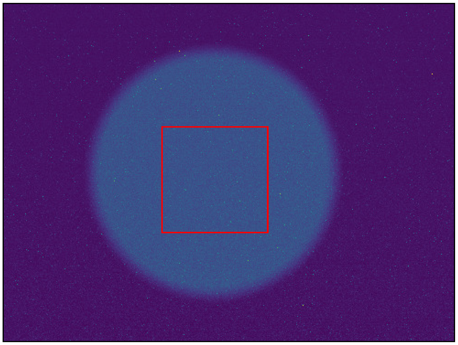
Figure 1.
Example region of interest (red rectangle) from relative spectral response data set. Pixels from center of sphere (exit port of mini integrating sphere) were averaged for every image captured. This was accomplished for all 250 images captured (400 nm–900 nm, 2 nm step size) for all bands.
Figure 1.
Example region of interest (red rectangle) from relative spectral response data set. Pixels from center of sphere (exit port of mini integrating sphere) were averaged for every image captured. This was accomplished for all 250 images captured (400 nm–900 nm, 2 nm step size) for all bands.
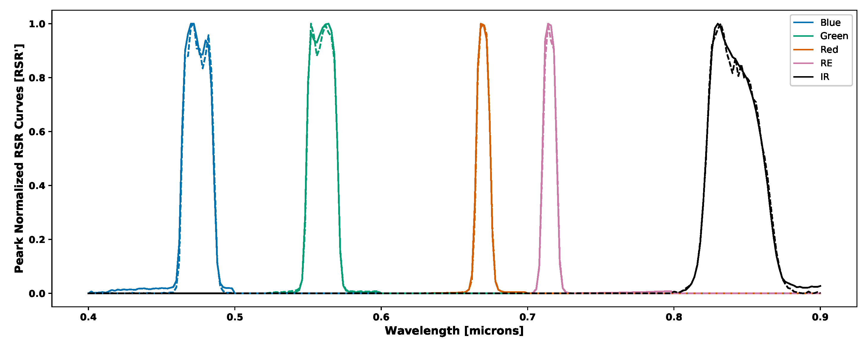
Figure 2.
Peak normalized relative spectral response of RedEdge-3 (solid lines) and RedEdge-M (dashed lines) sensors. Small variations can be seen in all channels of both sensors. RedEdge-3 contains small divots in the blue and green channels, while the Red, RE and NIR channels have small but noticeable shifts between the two sensors.
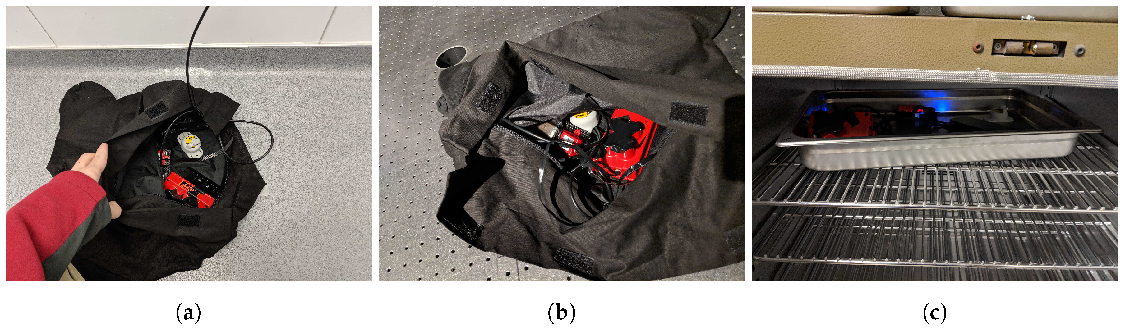
Figure 3.
MicaSense RedEdge-3 and HOBO TidbiT MX Temp 400 during dark current testing in (a) cold room, (b) room temperature and (c) bench oven.
Figure 3.
MicaSense RedEdge-3 and HOBO TidbiT MX Temp 400 during dark current testing in (a) cold room, (b) room temperature and (c) bench oven.
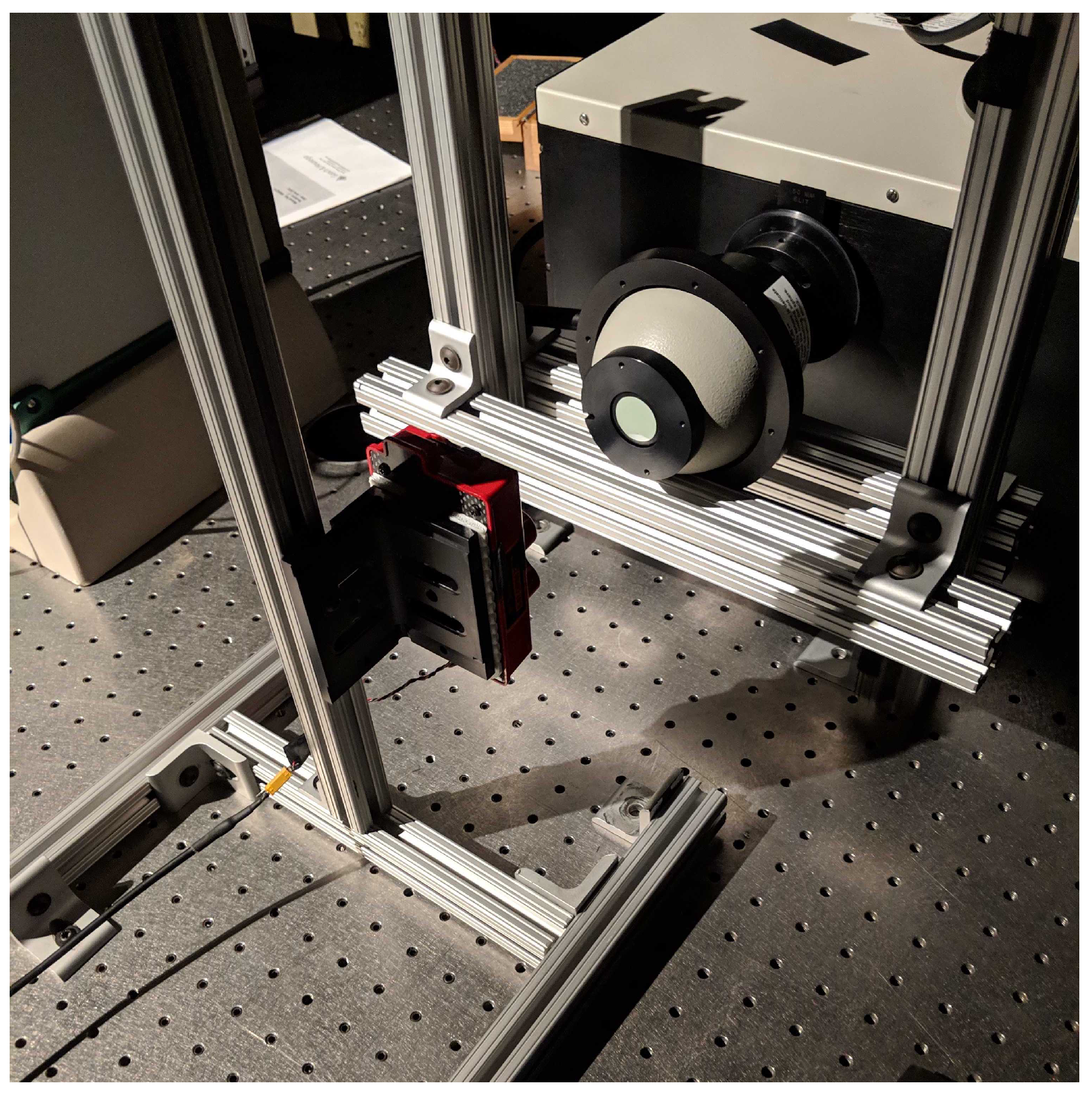
Figure 4.
Relative spectral response curve data capture setup. Monochromator exit port connected to mini integrating sphere. RedEdge-3’s center lens is aligned with exit port of mini sphere. RedEdge-3 is attached to a custom made rig which allowed for both lateral and vertical movement.
Figure 4.
Relative spectral response curve data capture setup. Monochromator exit port connected to mini integrating sphere. RedEdge-3’s center lens is aligned with exit port of mini sphere. RedEdge-3 is attached to a custom made rig which allowed for both lateral and vertical movement.
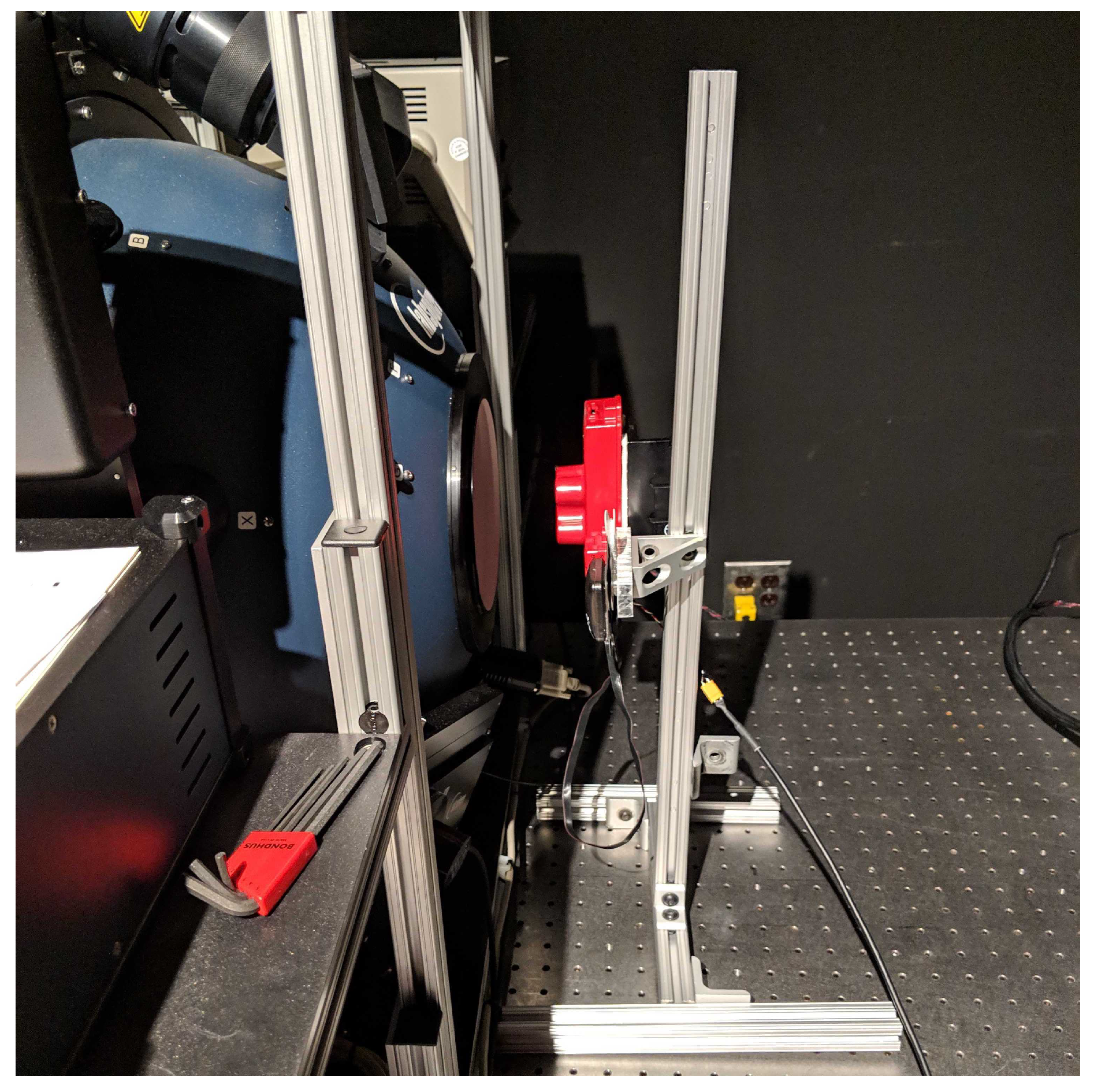
Figure 5.
Radiometric calibration data capture setup. RedEdge-3 sensor is placed in front of the exit port of the integrating sphere. Sensor is placed far enough away to avoid stray light issues but close enough for all channels to be completely filled. RedEdge is attached to a custom made rig which allowed for both lateral and vertical movement.
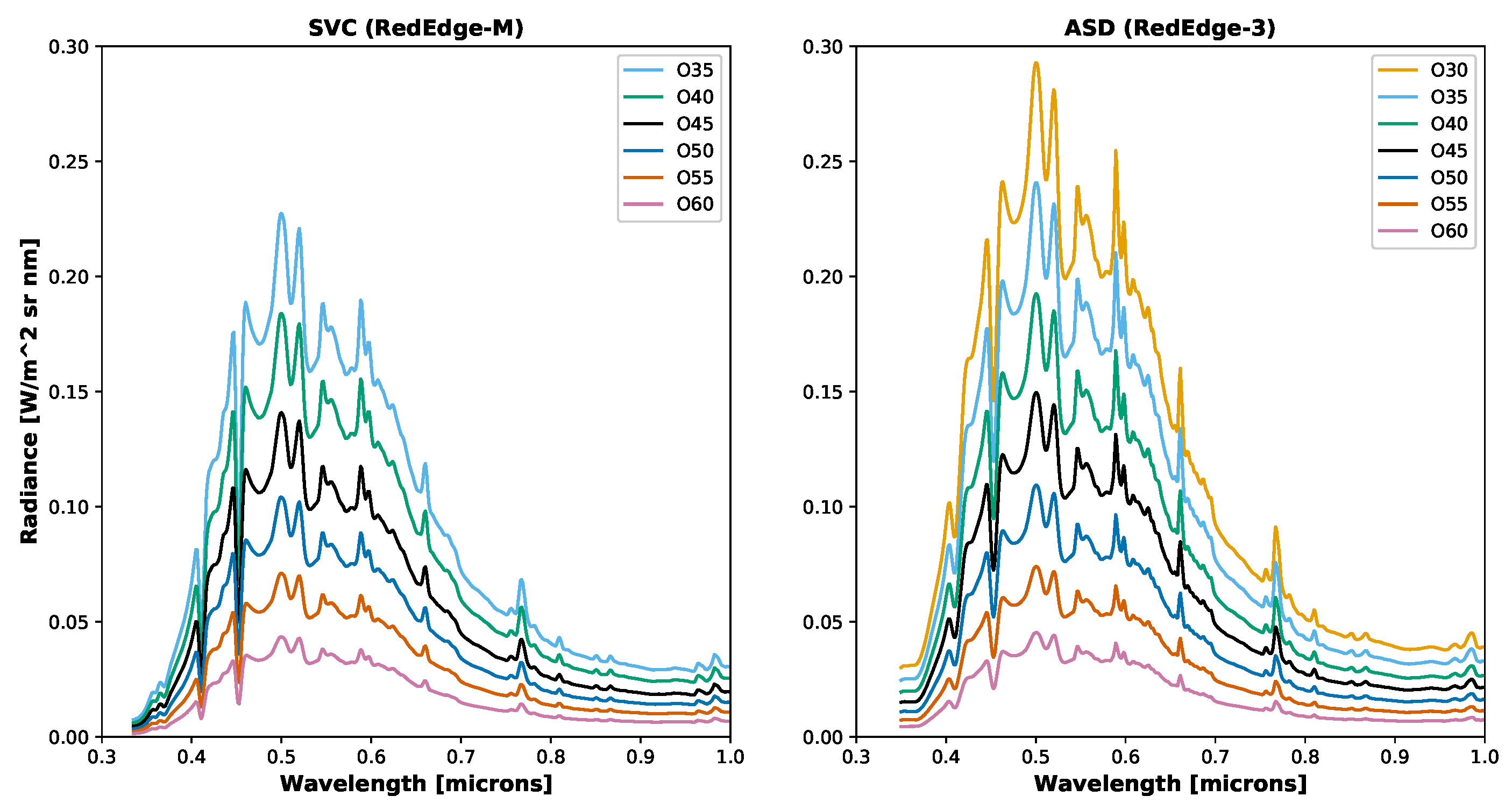
Figure 6.
Example integrating sphere radiances. (Left) SVC radiances collected and used for calibrating the RedEdge-M sensor. (Right) ASD radiances collected and used for calibrating the RedEdge-3 sensor. As expected, the measured spectra decreased in magnitude as the PEL’s aperture was closed.
Figure 6.
Example integrating sphere radiances. (Left) SVC radiances collected and used for calibrating the RedEdge-M sensor. (Right) ASD radiances collected and used for calibrating the RedEdge-3 sensor. As expected, the measured spectra decreased in magnitude as the PEL’s aperture was closed.
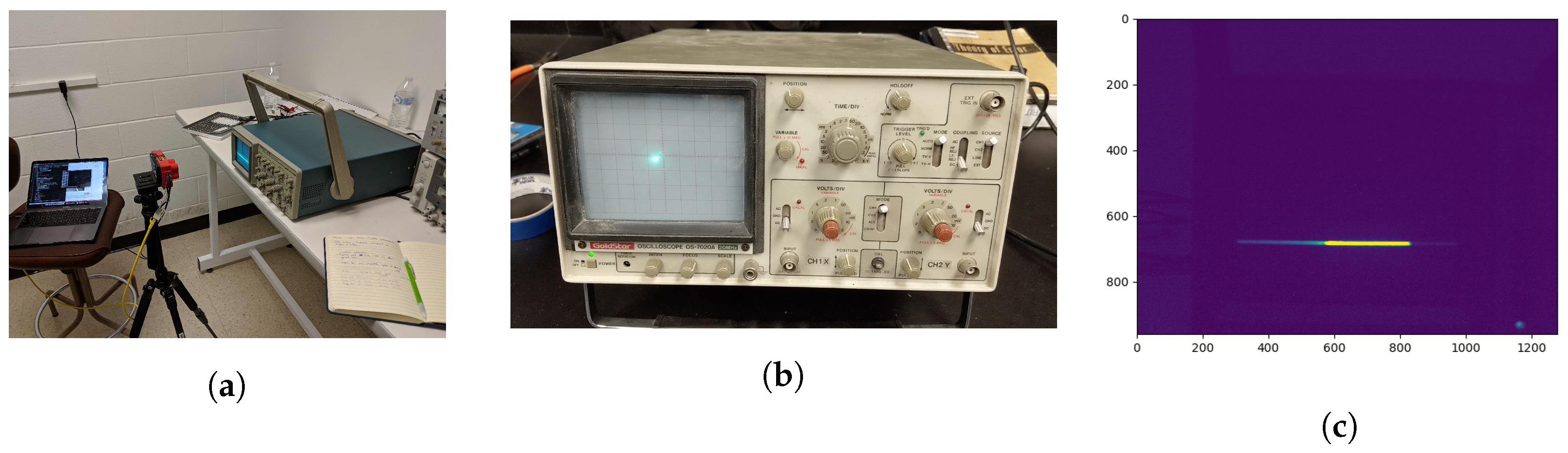
Figure 7.
Exposure time error (a) setup, (b) example oscilloscope dot and (c) example RedEdge image. Images were used for analysis if the full line was imaged in the center of the frame. This ensures the proper exposure time could be measured.
Figure 7.
Exposure time error (a) setup, (b) example oscilloscope dot and (c) example RedEdge image. Images were used for analysis if the full line was imaged in the center of the frame. This ensures the proper exposure time could be measured.
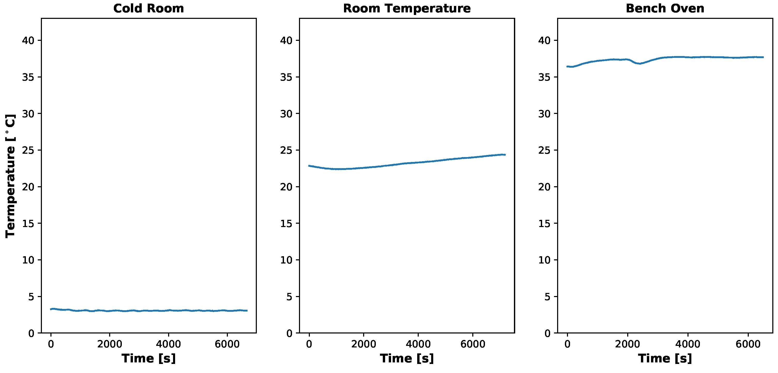
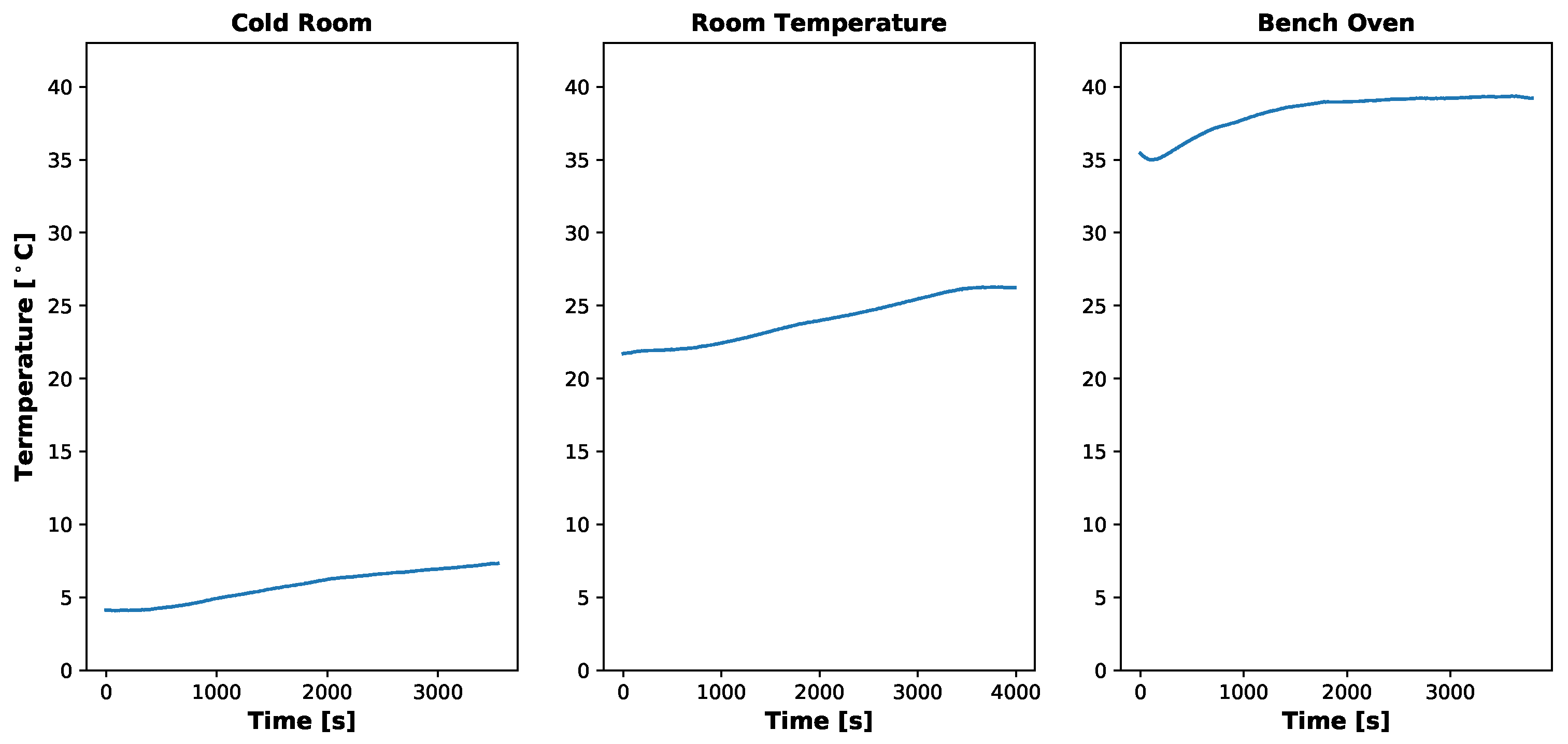
Figure 8.
Temporal temperature profile during MicaSense RedEdge-3 dark current testing. Temperature inside the light tight bag did not change significantly during the course of the test. Data collection took about 2 h for each temperature environment because the gain and exposure time had to be changed manually in-between image captures.
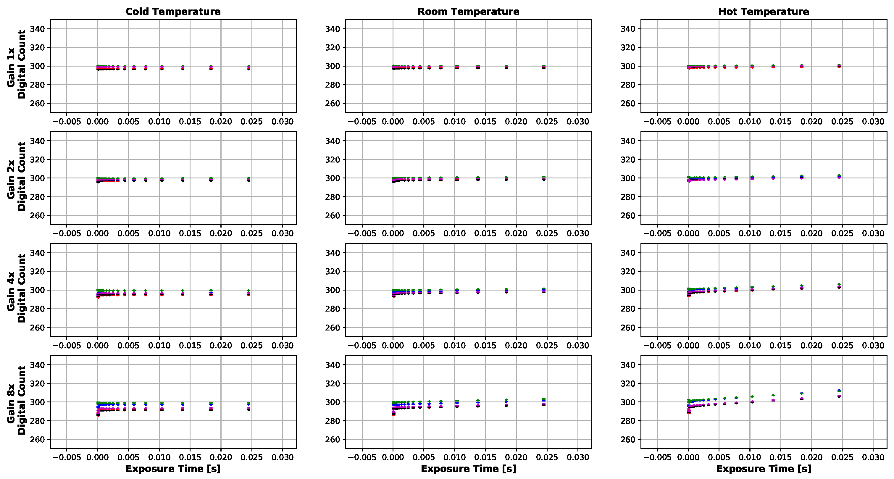
Figure 9.
Average dark current (12-bit) produced by MicaSense RedEdge-3 sensor at various gains and exposure times. Each dot represents an average of at least 30 images. Bars are one standard deviation. Digital count values hold around 300 except for higher exposure times, gains and temperatures. The highest digital counts values seen were around 340 (24.5 ms, 8× gain and 37.22 C).
Figure 10.
Temporal temperature profile during MicaSense RedEdge-M dark current testing. Temperature inside light tight bag did rise as test progressed but no significant changes in the digital counts were noticed. Data collection took about an hour for each temperature setting because the gain and exposure time were altered programatically using the RedEdge Application Program Interface (API).
Figure 11.
Average dark current (12-bit) produced by MicaSense RedEdge-M sensor at various gains and exposure times. Each dot represents an average of at least 30 images. Bars are one standard deviation. Digital count values hold around 300 except for higher exposure times, gains and temperatures. The highest digital counts values seen were around 320 (24.5 ms, 8× gain and 37.22 C). It should also be noted that the digital count values held steady regardless of the increasing temperature throughout the test.
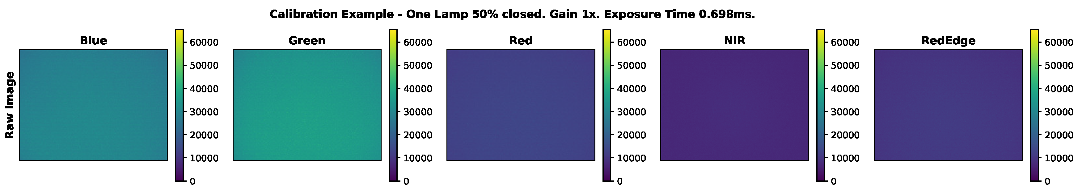
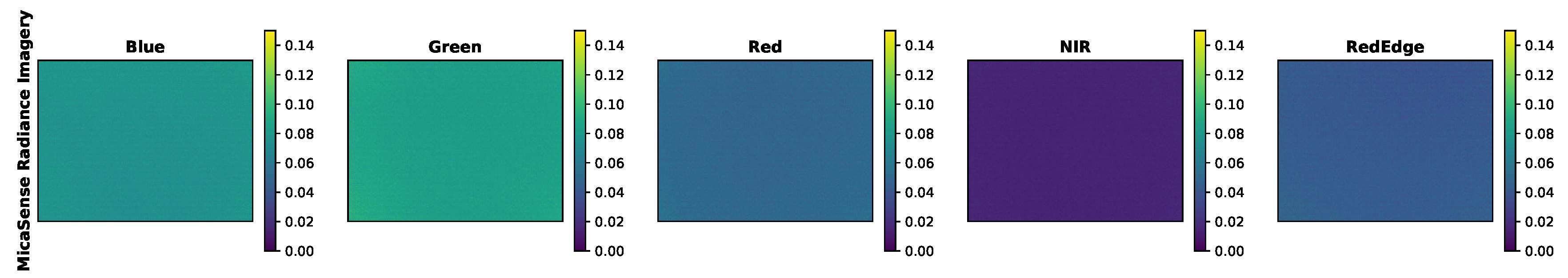
Figure 12.
Example raw RedEdge imagery taken of the integrating sphere during calibration testing.
Figure 12.
Example raw RedEdge imagery taken of the integrating sphere during calibration testing.
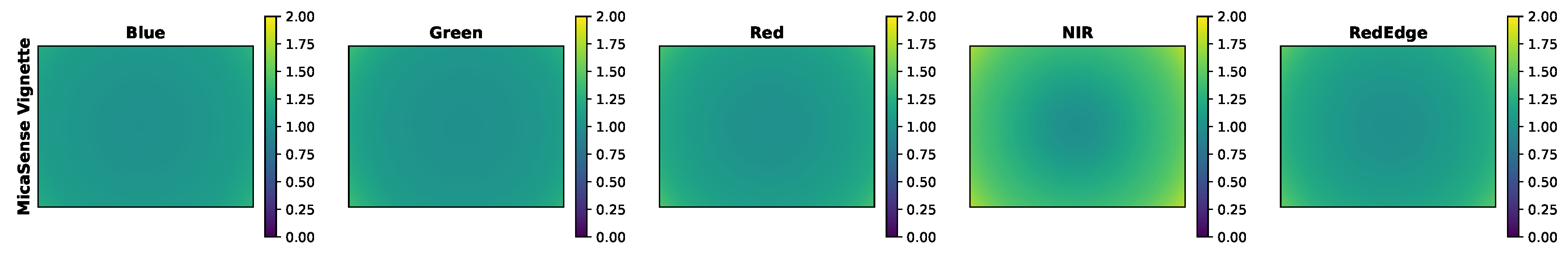
Figure 13.
MicaSense vignette imagery. These vignettes are programmed into the particular MicaSense RedEdge-3 sensor used in this study and will never change throughout the lifetime of the sensor.
Figure 13.
MicaSense vignette imagery. These vignettes are programmed into the particular MicaSense RedEdge-3 sensor used in this study and will never change throughout the lifetime of the sensor.
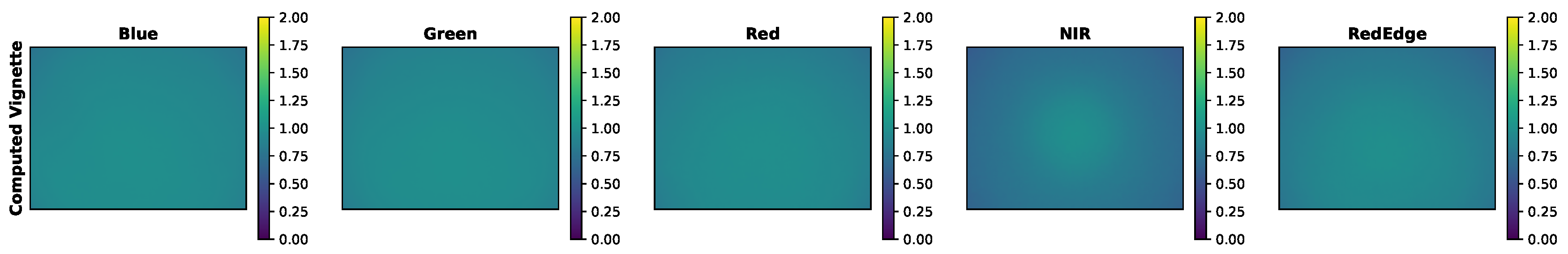
Figure 14.
Example proposed vignettes. These vignettes are computed with the methodology proposed in this paper, for the particular light level, gain and exposure time combination (One Lamp 50% closed, Gain 2× and 0.698 ms).
Figure 14.
Example proposed vignettes. These vignettes are computed with the methodology proposed in this paper, for the particular light level, gain and exposure time combination (One Lamp 50% closed, Gain 2× and 0.698 ms).
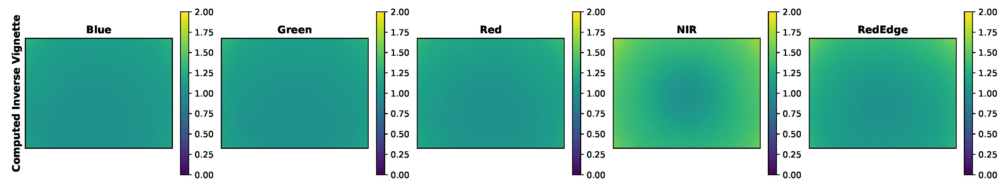
Figure 15.
Inverse of example proposed vignettes. Proposed methodology divides the image by the vignette, while MicaSense method multiples. These images were produced to showcase the similarity between MicaSense and proposed vignettes.
Figure 15.
Inverse of example proposed vignettes. Proposed methodology divides the image by the vignette, while MicaSense method multiples. These images were produced to showcase the similarity between MicaSense and proposed vignettes.
Figure 16.
Example integrating sphere imagery converted into radiance using MicaSense radiance methodology. 3-D images are shown below for clarity.
Figure 16.
Example integrating sphere imagery converted into radiance using MicaSense radiance methodology. 3-D images are shown below for clarity.
Figure 17.
Example integrating sphere imagery converted into radiance using proposed technique. 3-D images are shown below for clarity.
Figure 17.
Example integrating sphere imagery converted into radiance using proposed technique. 3-D images are shown below for clarity.
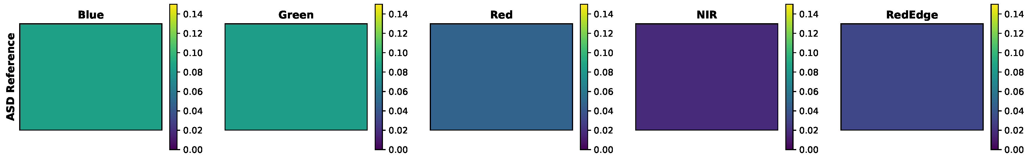
Figure 18.
ASD reference values measured of the integrating sphere during calibration testing. RedEdge-3 RSR curves applied to ASD spectra to compute band integrated radiances, which are being displayed as images.
Figure 18.
ASD reference values measured of the integrating sphere during calibration testing. RedEdge-3 RSR curves applied to ASD spectra to compute band integrated radiances, which are being displayed as images.
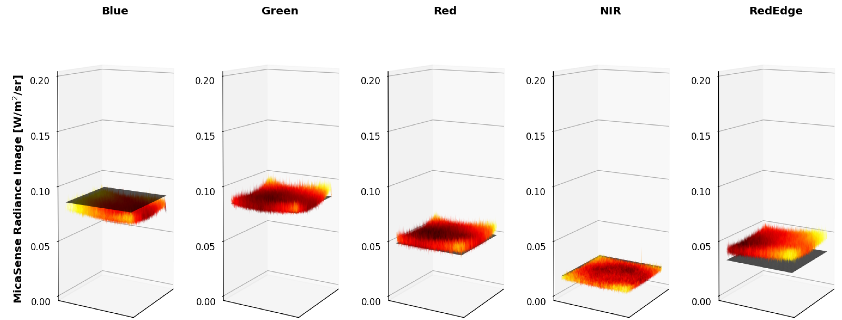
Figure 19.
Example MicaSense radiance imagery shown as 3-D images. ASD reference is shown as a black 2-D image. Imperfections of MicaSense methodology is noticeable in the magnitude (radiance calibration coefficients) and in the edges (vignette correction) of the radiance images.
Figure 19.
Example MicaSense radiance imagery shown as 3-D images. ASD reference is shown as a black 2-D image. Imperfections of MicaSense methodology is noticeable in the magnitude (radiance calibration coefficients) and in the edges (vignette correction) of the radiance images.
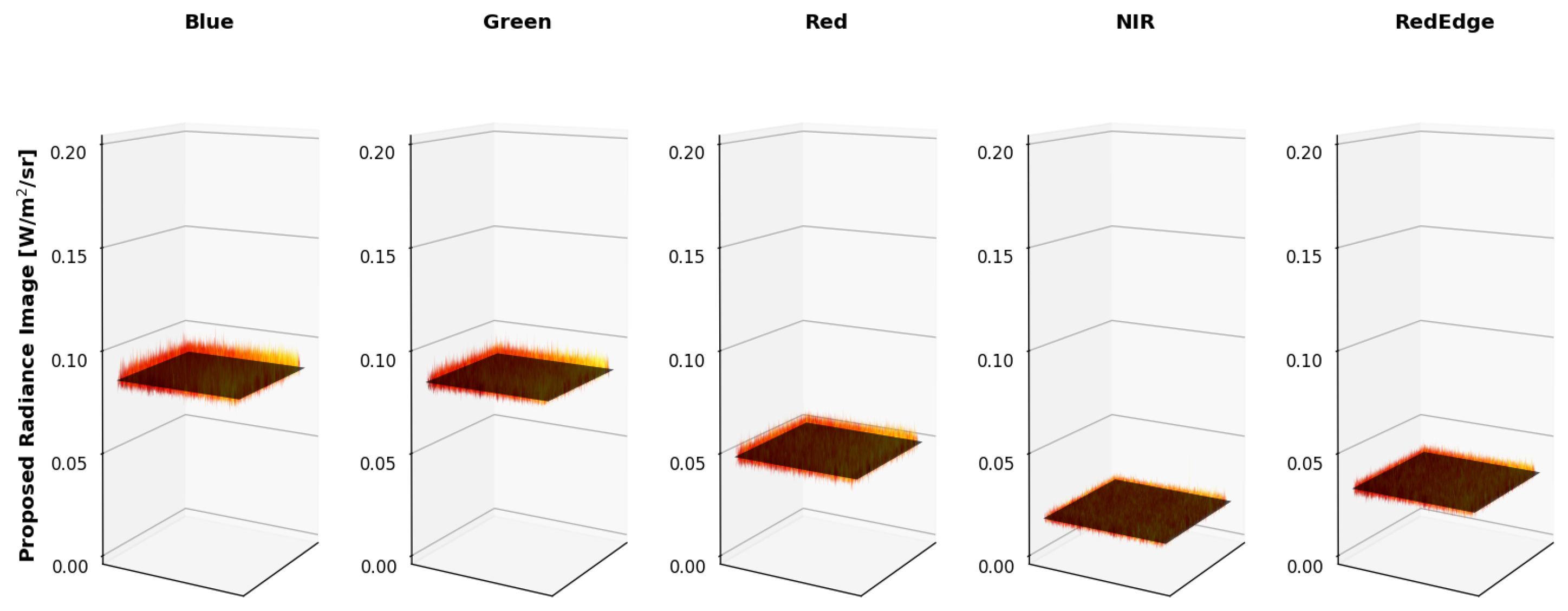
Figure 20.
Example proposed radiance imagery shown as 3-D images. ASD reference is shown as a black 2-D image. Using the proposed methodology, the produced radiance imagery magnitudes line up with the ASD reference and the applied vignette correction flattened the images.
Figure 20.
Example proposed radiance imagery shown as 3-D images. ASD reference is shown as a black 2-D image. Using the proposed methodology, the produced radiance imagery magnitudes line up with the ASD reference and the applied vignette correction flattened the images.
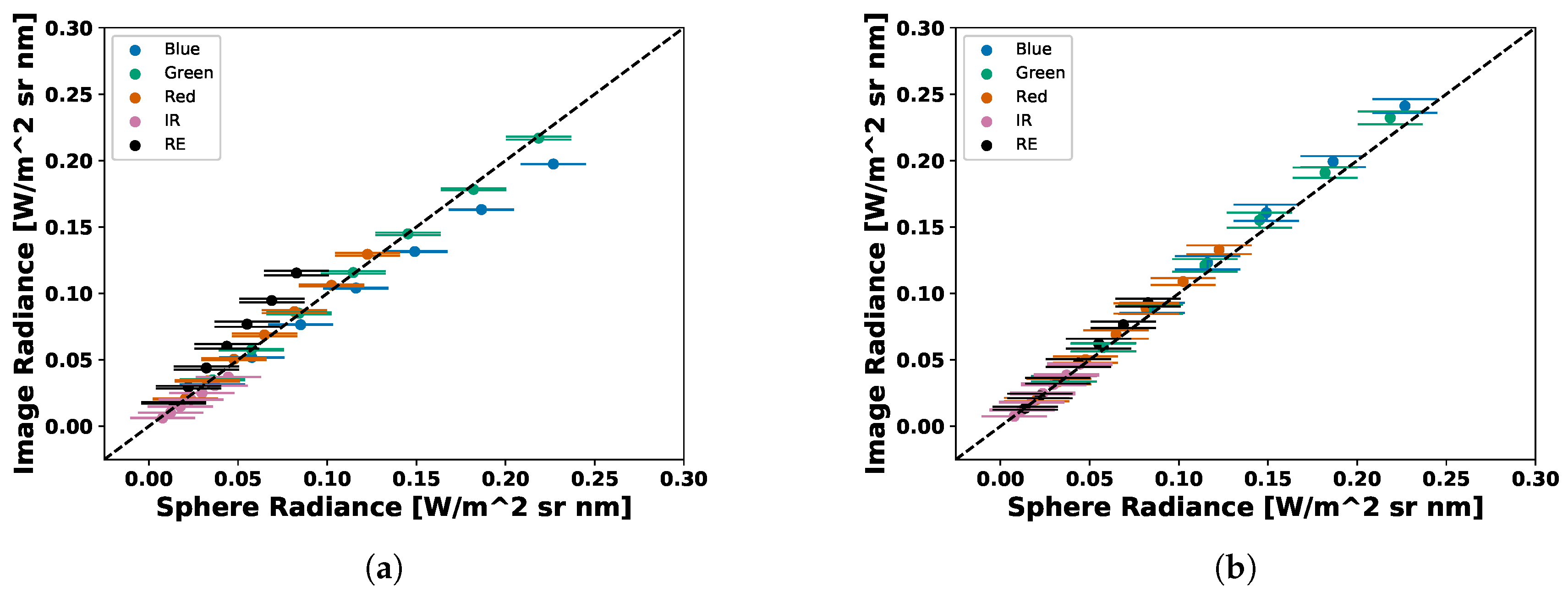
Figure 21.
Scatter plot of average RedEdge-3 image radiance vs sphere radiance. Images converted to radiance using (a) MicaSense methodology (b) Average Vignette Proposed methodology. Proposed methodology produces less error as less spread is seen in the scatter plot.
Figure 21.
Scatter plot of average RedEdge-3 image radiance vs sphere radiance. Images converted to radiance using (a) MicaSense methodology (b) Average Vignette Proposed methodology. Proposed methodology produces less error as less spread is seen in the scatter plot.
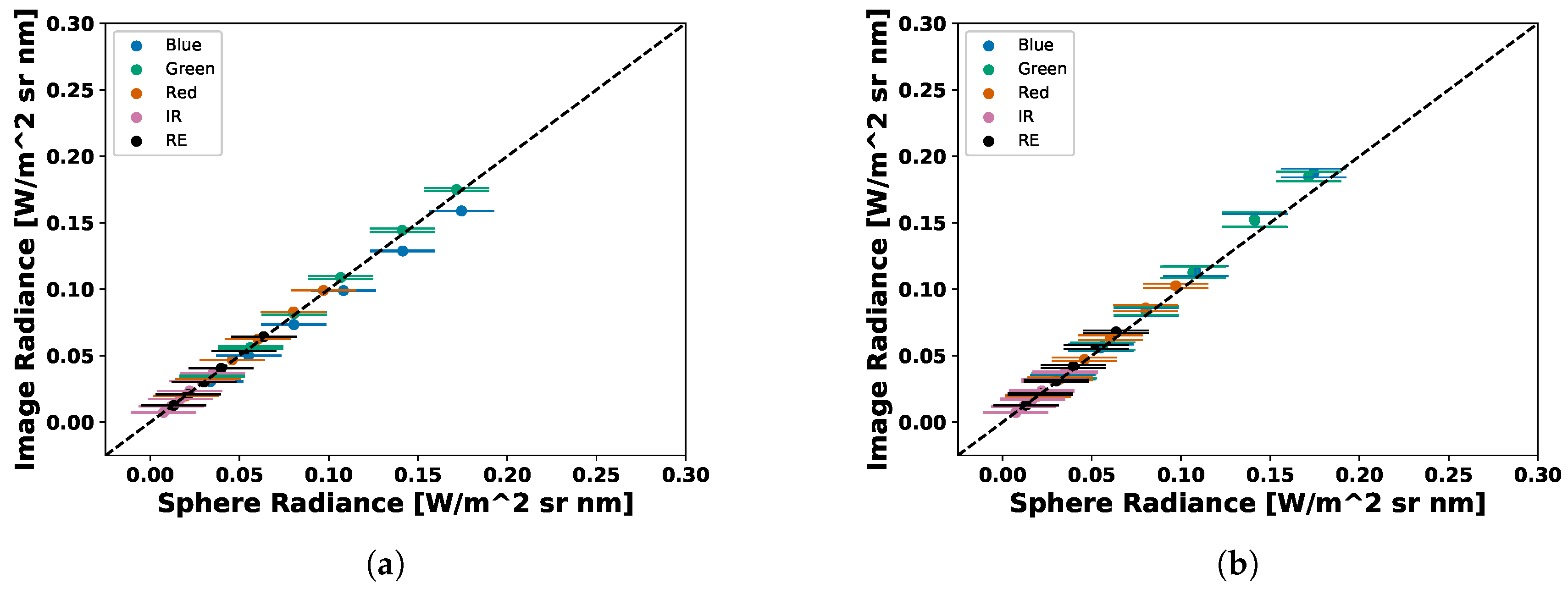
Figure 22.
Scatter plot of average RedEdge-M image radiance vs sphere radiance. Images converted to radiance using (a) MicaSense methodology (b) Average Vignette Proposed methodology. Proposed methodology produces less error as less spread is seen in the scatter plot.
Figure 22.
Scatter plot of average RedEdge-M image radiance vs sphere radiance. Images converted to radiance using (a) MicaSense methodology (b) Average Vignette Proposed methodology. Proposed methodology produces less error as less spread is seen in the scatter plot.
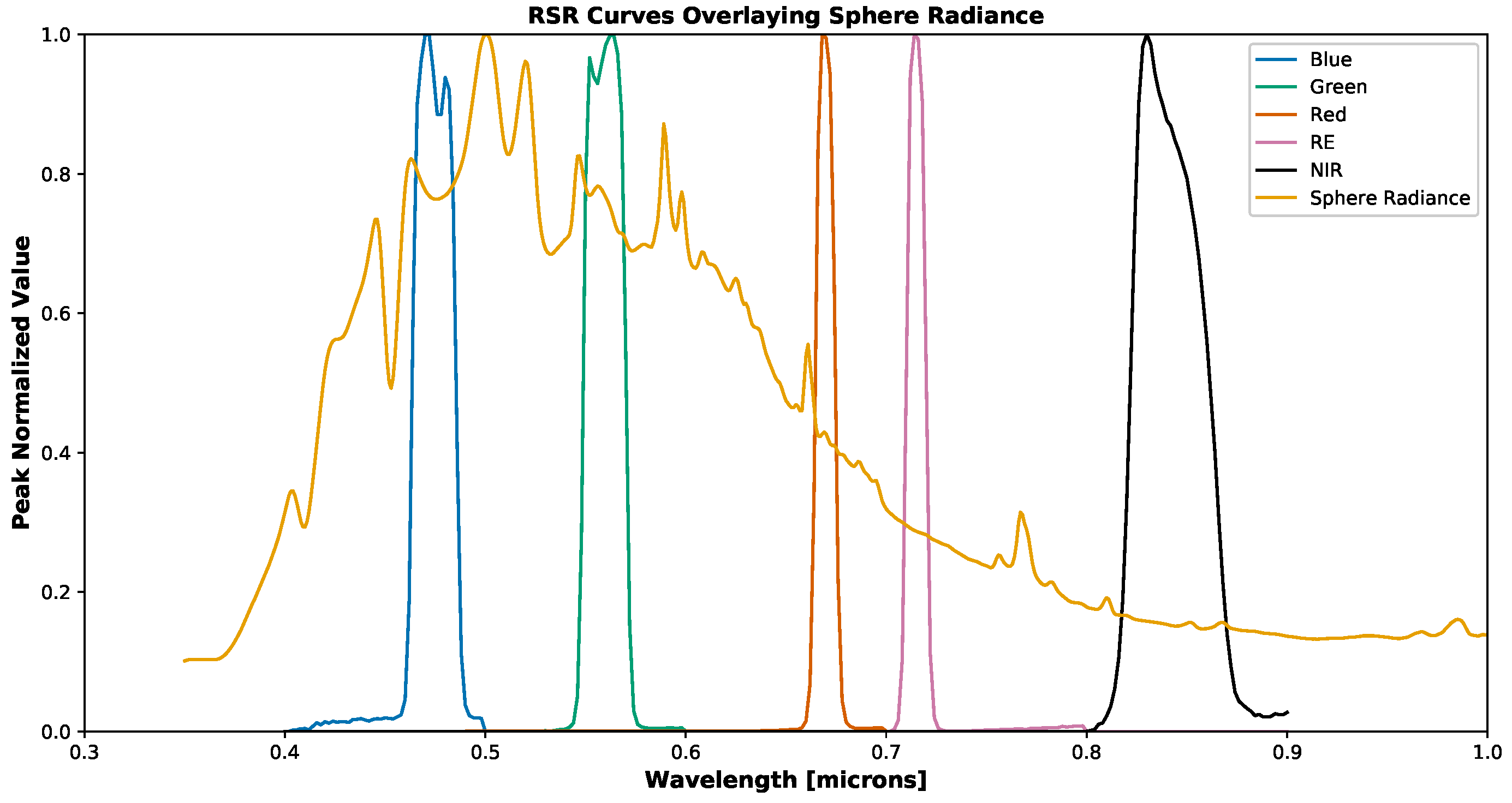
Figure 23.
Peak normalized MicaSense RedEdge-3 RSR curves overlaid onto normalized spectral radiance curve.
Figure 23.
Peak normalized MicaSense RedEdge-3 RSR curves overlaid onto normalized spectral radiance curve.
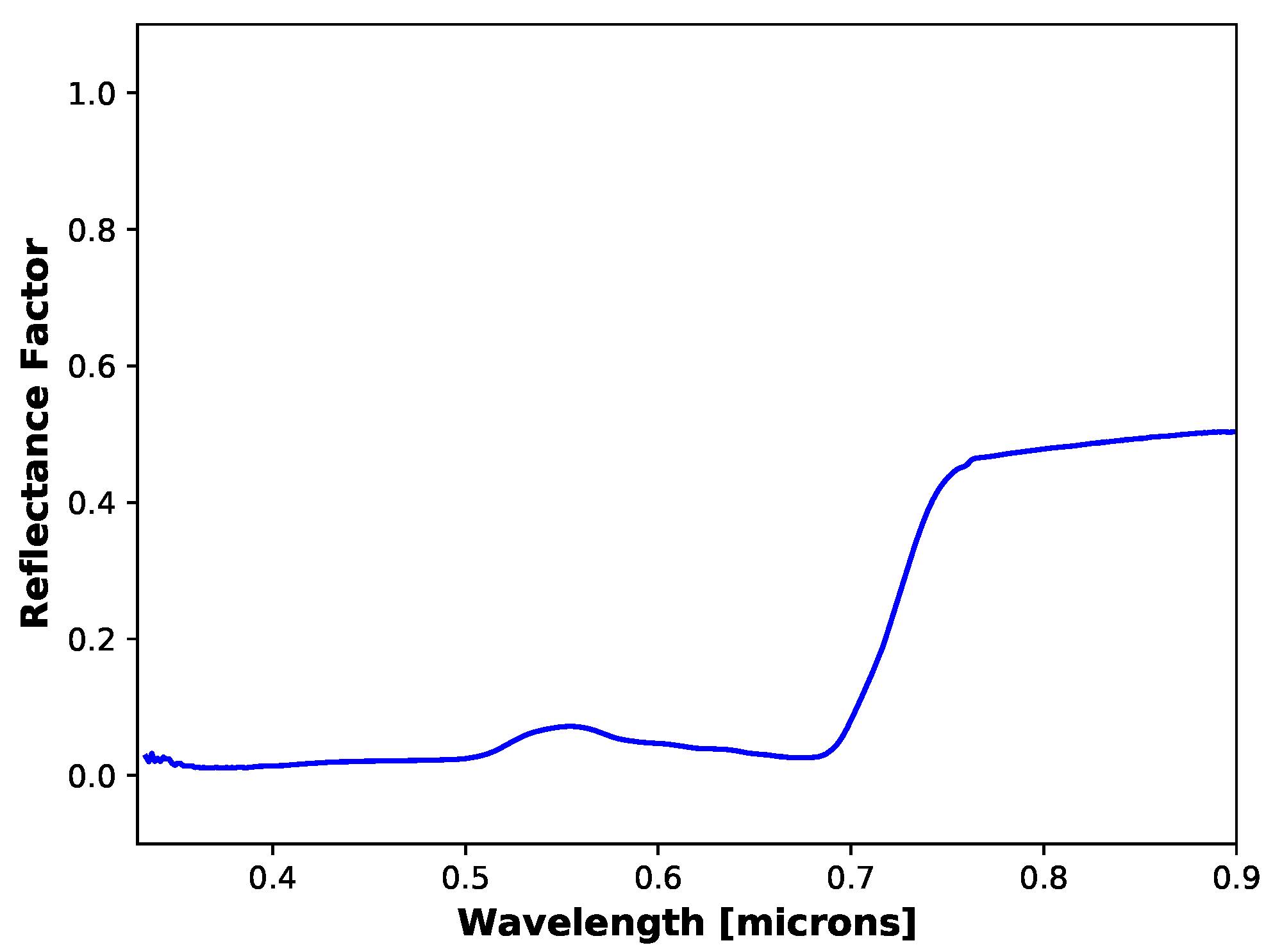
Figure 24.
Ground reference reflectance of grass target measured with SVC during a field collection in 2018. This measurement is a single measurement of the grass target.
Figure 24.
Ground reference reflectance of grass target measured with SVC during a field collection in 2018. This measurement is a single measurement of the grass target.
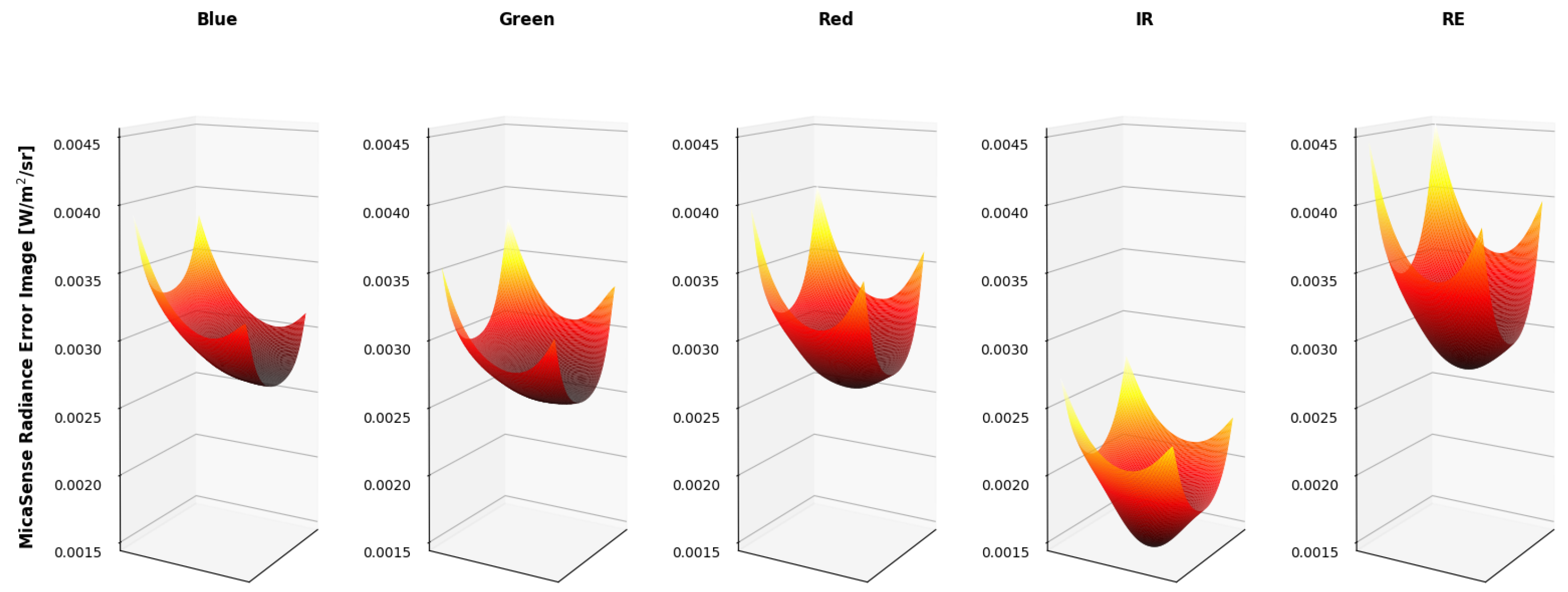
Figure 25.
Example error of MicaSense radiance imagery. Only gain, exposure time and image error components are present in these errors. Noticeable vignette shape is seen in all channels.
Figure 25.
Example error of MicaSense radiance imagery. Only gain, exposure time and image error components are present in these errors. Noticeable vignette shape is seen in all channels.
Figure 26.
Error of proposed radiance imagery. Gain, exposure time, image and radiometric calibration coefficient error components are present. Error images are all flat for all channels, as the radiance images were.
Figure 26.
Error of proposed radiance imagery. Gain, exposure time, image and radiometric calibration coefficient error components are present. Error images are all flat for all channels, as the radiance images were.
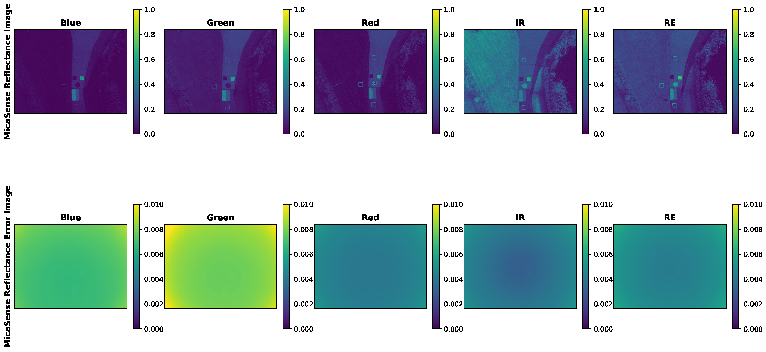
Figure 27.
Example sUAS reflectance factor image and reflectance factor error image. Radiance image computed using MicaSense methodology and AARR used to compute reflectance factor. Reflectance factor error only contains gain, exposure time, image and DLS error. Error image is overwhelmed by the vignette shape. Reflectance factor is a unit-less quantity.
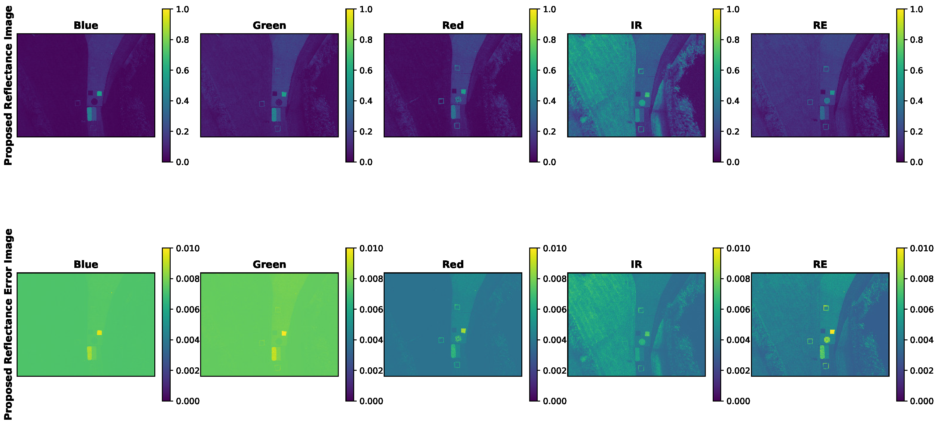
Figure 28.
Example sUAS reflectance factor image and reflectance factor error image. Radiance image computed using proposed methodology and AARR used to compute reflectance factor. Reflectance factor error contains gain, exposure time, image, radiometric calibration coefficient and dls error. Error image contains same features as the reflectance factor image (concrete path, grass, demarcated targets and reflectance conversion panels). Reflectance factor is a unit-less quantity.
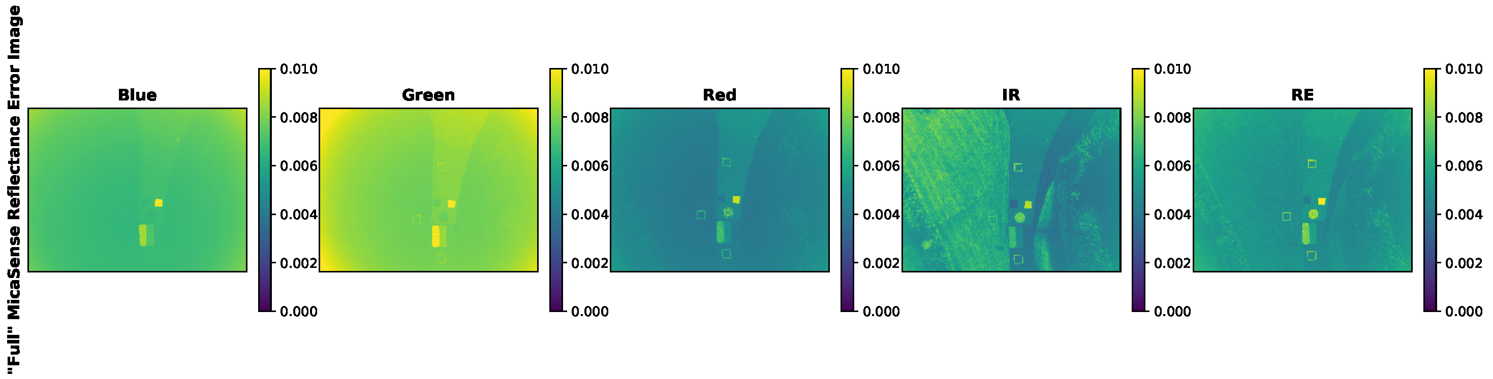
Figure 29.
Example sUAS reflectance error image. Error image contains the measured gain, exposure time, image and dls error. While the vignette and radiometric calibration coefficient standard errors were set to 1% of their values. These error images produce the same features as the reflectance image and the proposed methodology reflectance error images. Reflectance factor is a unit-less quantity.
Table 1.
MicaSense RedEdge spectral bands with respective center wavelengths and bandwidth values.
Table 1.
MicaSense RedEdge spectral bands with respective center wavelengths and bandwidth values.
| Band Name | Wavelengths [nm] | FWHM [nm] |
|---|
| Blue | 475 | 20 |
| Green | 560 | 20 |
| Red | 668 | 10 |
| Red Edge | 717 | 10 |
| Near IR | 840 | 40 |
Table 2.
Band integrated sphere radiances. Values were computed by applying RedEdge-3 RSR curves to the measured sphere radiances. All spectral band columns have units of W/m/sr/nm.
Table 2.
Band integrated sphere radiances. Values were computed by applying RedEdge-3 RSR curves to the measured sphere radiances. All spectral band columns have units of W/m/sr/nm.
| % Closed | Peak Radiance [W/m/sr/nm] | Blue | Green | Red | NIR | RedEdge |
|---|
| 30 | 0.2928 | 0.2268 | 0.2186 | 0.1226 | 0.0445 | 0.0827 |
| 35 | 0.2407 | 0.1865 | 0.1820 | 0.1024 | 0.0371 | 0.0689 |
| 40 | 0.1924 | 0.1491 | 0.1453 | 0.0817 | 0.0298 | 0.0551 |
| 45 | 0.1495 | 0.1161 | 0.1146 | 0.0648 | 0.0237 | 0.0437 |
| 50 | 0.1093 | 0.0851 | 0.0842 | 0.0477 | 0.0176 | 0.0322 |
| 55 | 0.0739 | 0.0578 | 0.0575 | 0.0327 | 0.0122 | 0.0222 |
| 60 | 0.0453 | 0.0355 | 0.0357 | 0.0204 | 0.0077 | 0.0139 |
Table 3.
Radiometric calibration coefficients computed using proposed methodology for both RedEdge-3 and RedEdge-M sensors. The Blue, Green and Red bands produced very similar coefficients, while the NIR and RedEdge bands were different.
Table 3.
Radiometric calibration coefficients computed using proposed methodology for both RedEdge-3 and RedEdge-M sensors. The Blue, Green and Red bands produced very similar coefficients, while the NIR and RedEdge bands were different.
| | Blue | Green | Red | NIR | RedEdge |
|---|
| RedEdge-3 | 3.656 × | 2.916 × | 5.863 × | 5.168 × | 5.396 × |
| RedEdge-M | 3.233 × | 2.814 × | 5.698 × | 3.726 × | 6.524 × |
Table 4.
Average percent errors in radiance imagery for all bands using both conversion methods for the RedEdge-3. Standard deviations are shown in parenthesis.
Table 4.
Average percent errors in radiance imagery for all bands using both conversion methods for the RedEdge-3. Standard deviations are shown in parenthesis.
| Sensor | Method | Blue | Green | Red | RedEdge | NIR |
|---|
| RedEdge-3 | MicaSense | −10.98 (0.93) | −0.43 (1.59) | 3.59 (2.67) | 32.81 (5.94) | −17.08 (2.45) |
| Proposed (Average) | 3.44 (5.63) | 2.93 (5.47) | 2.93 (6.63) | 3.70 (8.91) | 0.72 (4.08) |
| Proposed (Closest) | 3.66 (6.05) | 3.19 (5.95) | 3.25 (7.17) | 4.23 (9.74) | 0.75 (3.95) |
Table 5.
Average percent errors in radiance imagery for all bands using both conversion methods for the RedEdge-M. Standard deviations are shown in parenthesis.
Table 5.
Average percent errors in radiance imagery for all bands using both conversion methods for the RedEdge-M. Standard deviations are shown in parenthesis.
| Sensor | Method | Blue | Green | Red | RedEdge | NIR |
|---|
| RedEdge-M | MicaSense | −9.22 (0.61) | 0.50 (1.70) | 0.82 (1.79) | −1.62 (2.72) | 1.58 (3.66) |
| Proposed (Average) | 2.50 (4.82) | 2.91 (5.34) | 1.28 (4.31) | 0.99 (4.51) | 0.78 (5.05) |
| Proposed (Closest) | 2.82 (5.41) | 3.14 (5.78) | 1.70 (5.01) | 1.10 (4.55) | 0.78 (4.86) |
Table 6.
Grass target reflectance factor errors as a result of calibration errors.
Table 6.
Grass target reflectance factor errors as a result of calibration errors.
| Sensor | Method | Blue | Green | Red | RedEdge | NIR | NDVI | NDRE |
|---|
| SVC | Reference | 0.022 | 0.071 | 0.026 | 0.188 | 0.490 | 0.899 | 0.445 |
| RedEdge-3 | MicaSense Correction | 0.020 | 0.070 | 0.027 | 0.249 | 0.406 | 0.876 (0.005) | 0.239 (0.026) |
| Proposed Correction | 0.023 | 0.073 | 0.027 | 0.193 | 0.487 | 0.897 (0.007) | 0.435 (0.038) |
| RedEdge-M | MicaSense Correction | 0.020 | 0.071 | 0.026 | 0.185 | 0.491 | 0.899 (0.004) | 0.458 (0.018) |
| Proposed Correction | 0.022 | 0.073 | 0.026 | 0.189 | 0.491 | 0.898 (0.006) | 0.444 (0.027) |
Table 7.
RedEdge-3 12-bit digital count error for various light level, gain and exposure combinations. Digital count error was computed using vignette and row-corrected imagery from an integrating sphere. A positive correlation is seen between digital count error and both gain and exposure time, while a negative correlation is seen for digital count error and light level.
| % Closed | Peak Radiance | Exposures | Gain | Blue | Green | Red | NIR | RedEdge |
|---|
| [W/m/sr/nm] | [ms] |
|---|
| 50 | 0.1093 | 0.585 | 1 | 49.664 | 51.681 | 25.783 | 18.749 | 22.480 |
| 50 | 0.1093 | 0.585 | 2 | 98.905 | 102.491 | 51.271 | 36.732 | 44.843 |
| 55 | 0.0739 | 0.765 | 1 | 41.940 | 44.367 | 22.605 | 36.732 | 44.843 |
| 55 | 0.0739 | 0.765 | 2 | 83.420 | 88.443 | 44.711 | 34.432 | 39.722 |
| 60 | 0.0453 | 0.585 | 1 | 29.103 | 30.208 | 16.466 | 14.697 | 15.587 |
| 60 | 0.0453 | 0.585 | 2 | 57.727 | 59.945 | 32.609 | 28.981 | 30.257 |
| 60 | 0.0453 | 0.585 | 4 | 114.67 | 119.22 | 64.870 | 56.984 | 60.723 |
Table 8.
RedEdge-3 gain error for various light level, gain and exposure combinations. Digital count imagery was captured using an integrating sphere using a variety of light levels, gains and exposure times. Gain error was calculated by comparing the measured digital counts between images where the gain was the only variable difference.
| % Closed | Peak Radiance | Exposures | Gain Difference | Blue | Green | Red | NIR | RedEdge |
|---|
| [W/m/sr/nm] | [ms] |
|---|
| 50 | 0.1093 | 0.585 | 1× to 2× | 0.00022 | 0.00022 | 0.00027 | 0.00076 | 0.00043 |
| 55 | 0.0739 | 0.765 | 1× to 2× | 0.00014 | 0.00015 | 0.00023 | 0.00068 | 0.00053 |
| 60 | 0.0453 | 0.585 | 1× to 2× | 0.00025 | 0.00056 | 0.00078 | 0.00080 | 0.00121 |
| 60 | 0.0453 | 0.585 | 2× to 4× | 0.00029 | 0.00040 | 0.00049 | 0.00058 | 0.00074 |
| 60 | 0.0453 | 0.585 | 1× to 4× | 0.00055 | 0.00094 | 0.00140 | 0.00174 | 0.00262 |
Table 9.
RedEdge-3 exposure time errors for various settings. Errors were computed using an oscilloscope and measuring the line produced by a moving dot. A positive correlation can be seen between exposure time and error.
Table 9.
RedEdge-3 exposure time errors for various settings. Errors were computed using an oscilloscope and measuring the line produced by a moving dot. A positive correlation can be seen between exposure time and error.
| Exposure Time [ms] | Error |
|---|
| 0.5 | 2.7072 × |
| 1.0 | 4.5643 × |
| 2.5 | 1.0740 × |
Table 10.
RedEdge-3 radiometric calibration standard errors. Computed using the standard error for a regression estimate for all bands. Only 25 samples went into this computation, as the regression estimate itself contained only 25 samples.
Table 10.
RedEdge-3 radiometric calibration standard errors. Computed using the standard error for a regression estimate for all bands. Only 25 samples went into this computation, as the regression estimate itself contained only 25 samples.
| Blue | Green | Red | NIR | RedEdge |
|---|
| 3.988 × | 3.268 × | 8.118 × | 4.841 × | 1.062 × |
Table 11.
RedEdge-3 downwelling light sensor (DLS) standard errors. DLS measurements made using an integrating sphere at various light levels. Standard errors computed from 30 images at each light level. A positive correlation is seen between light level and the error.
Table 11.
RedEdge-3 downwelling light sensor (DLS) standard errors. DLS measurements made using an integrating sphere at various light levels. Standard errors computed from 30 images at each light level. A positive correlation is seen between light level and the error.
| % Closed | Peak Radiance | Blue | Green | Red | IR | RedEdge |
|---|
| [W/m/sr/nm] |
|---|
| 0 and 20 | 0.8023 | 3.6641 × | 2.1970 × | 1.1931 × | 4.6659 × | 8.8712 × |
| 0 and 40 | 0.6331 | 1.2486 × | 1.2858 × | 1.0518 × | 3.2586 × | 7.9633 × |
| 0 and 60 | 0.4989 | 2.9821 × | 3.0761 × | 3.8348 × | 1.0106 × | 2.3651 × |
| 0 and 80 | 0.4581 | 3.8725 × | 3.2880 × | 2.9041 × | 8.7316 × | 2.7989 × |
| 100 and 20 | 0.3585 | 7.2181 × | 6.6139 × | 5.0755 × | 1.5182 × | 3.7861 × |
| 100 and 40 | 0.1906 | 4.1037 × | 3.5980 × | 2.7043 × | 8.4237 × | 2.2069 × |
| 100 and 60 | 0.0449 | 1.0027 × | 1.4695 × | 6.4848 × | 3.5597 × | 1.0256 × |
| 100 and 80 | 0.0017 | 5.8776 × | 3.9563 × | 4.0075 × | 2.2207 × | 2.7876 × |
Table 12.
Percentage error in radiance of the radiance image. IR and RedEdge produced higher radiance errors under the MicaSense methodology.
Table 12.
Percentage error in radiance of the radiance image. IR and RedEdge produced higher radiance errors under the MicaSense methodology.
| Method | Blue | Green | Red | IR | RedEdge |
|---|
| MicaSense | 3.85 | 3.25 | 5.84 | 12.23 | 7.35 |
| Proposed | 3.75 | 3.21 | 5.45 | 9.29 | 6.54 |


