Spoofing Attack Results Determination in Code Domain Using a Spoofing Process Equation

Abstract
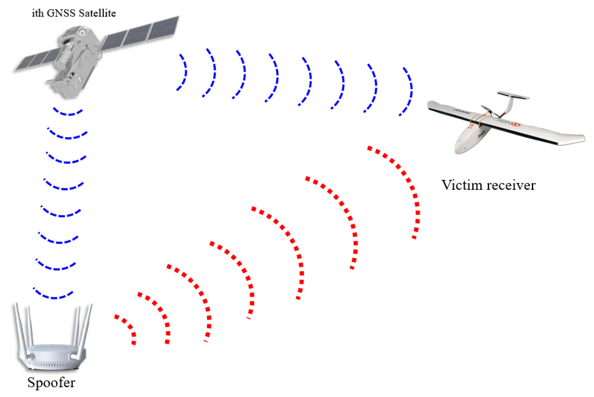
1. Introduction
- We develop an SPE that can be used to express the entire spoofing process in the form of an nth order polynomial.
- We obtain the spoofing results in one single calculation using the SPE and determine the correlation between each parameter based on the boundary line which distinguishes between successful and unsuccessful spoofing attacks.
- For a particular receiver, the minimum power of a spoofing signal for a successful spoofing attack could be estimated via the SPE.
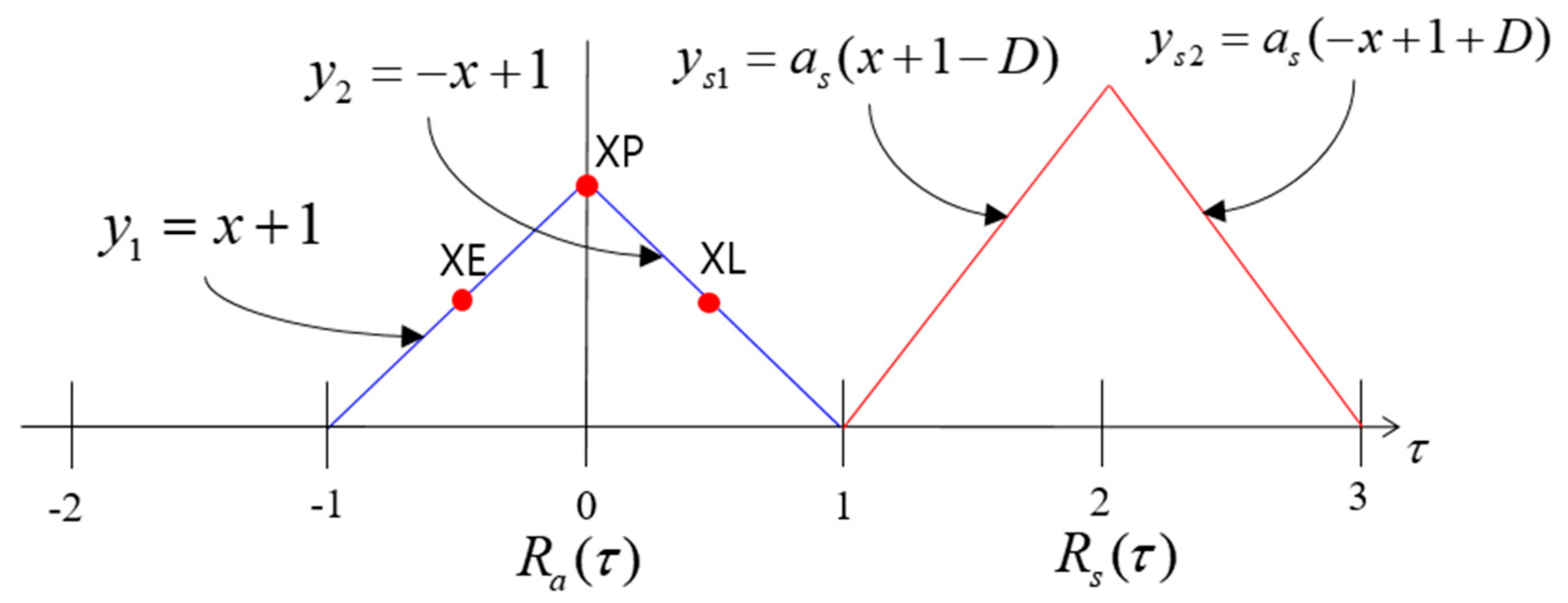
2. Authentic and Spoofing Signal ACF Model
- denotes the total received signal;
- denotes the pseudorandom code;
- is the code phase of the authentic signal;
- is the code phase of the spoofing signal;
- is the spoofing power advantage;
- is the carrier phase of the authentic signal;
- is the carrier phase of the spoofing signal;
- is the complex zero-mean white Gaussian noise (AWGN).
- indicates the left line of the ACF of the authentic signal;
- indicates the right line of the ACF of the authentic signal;
- is the ACF of the authentic signal;
- is the difference in the code phases between spoofing and authentic signals;
- indicates the left line of the ACF of the spoofing signal;
- indicates the right line of the ACF of the spoofing signal;
- is the slope of the ACF of the spoofing signal;
- is the ACF of the authentic signal;
- is the ACF of the total signal;
- XE is the accumulation result with the replica code separated 0.5 chip early;
- XP is the accumulation result with the replica code;
- XL is the accumulation result with the replica code separated 0.5 chip late.
- is the code phase difference between the local replica and the authentic signal;
- is the code phase difference between the local replica and the spoofing signal;
- is the Doppler frequency difference between the local replica and the authentic signal;
- is the Doppler frequency difference between the local replica and the spoofing signal;
- is the carrier phase difference between the local replica and the authentic signal;
- is the carrier phase difference between the local replica and the spoofing signal.
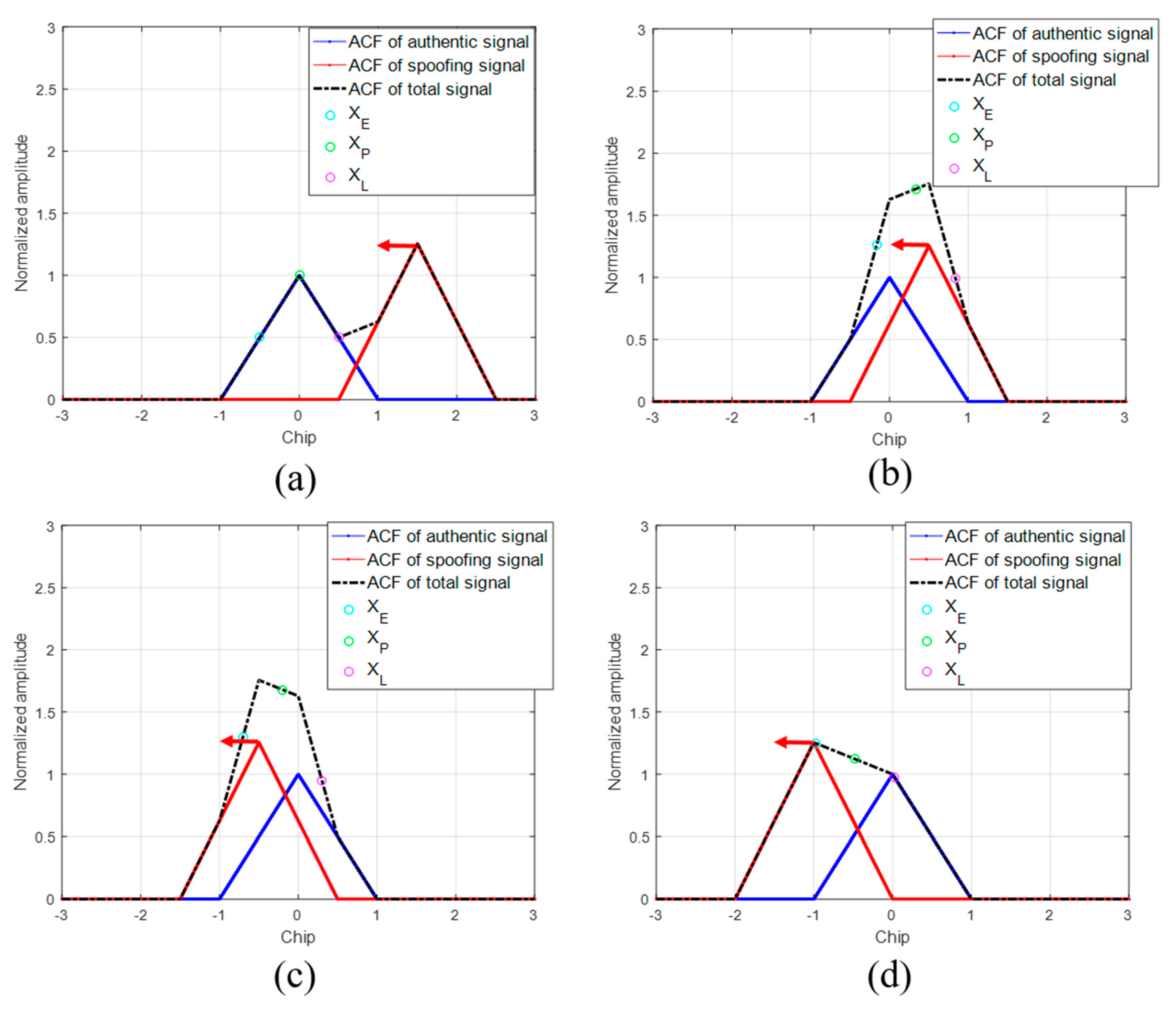
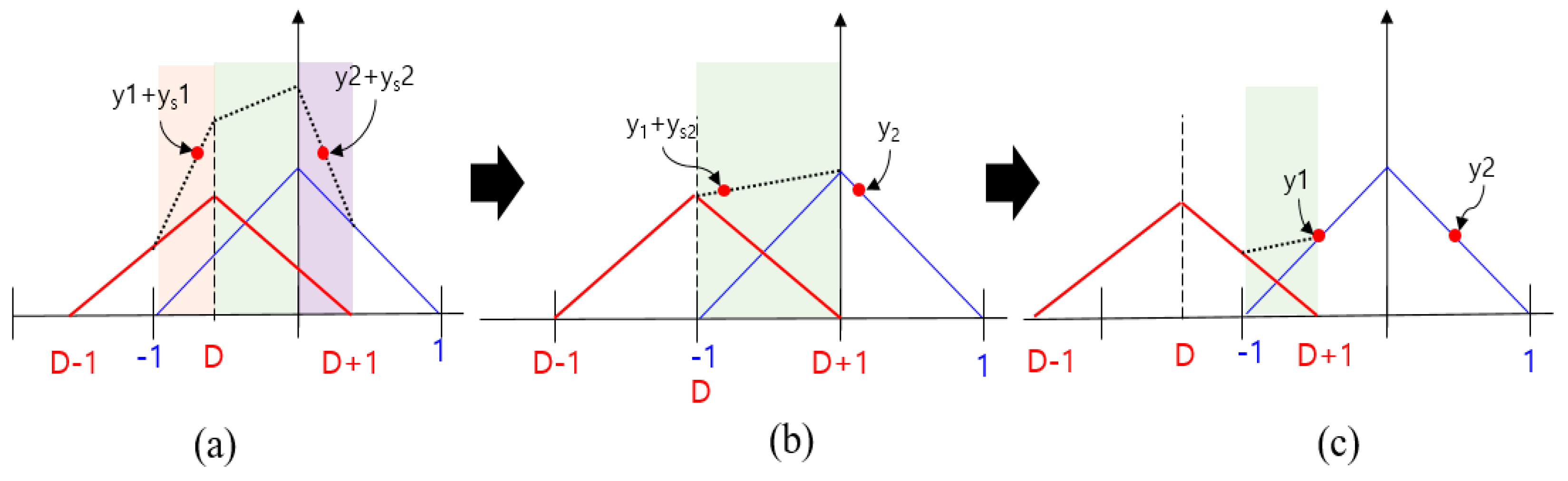
3. Spoofing Scenario Simulation Using ACF Model
4. Development of Spoofing Process Equation
4.1. Conventional Approach for τ Calculation
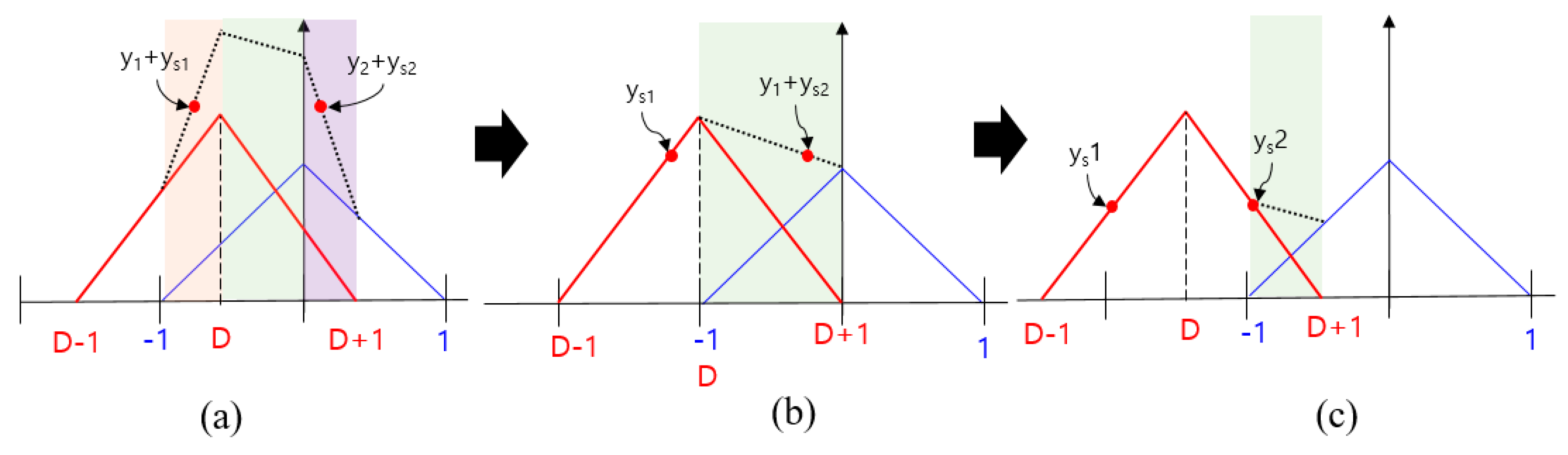
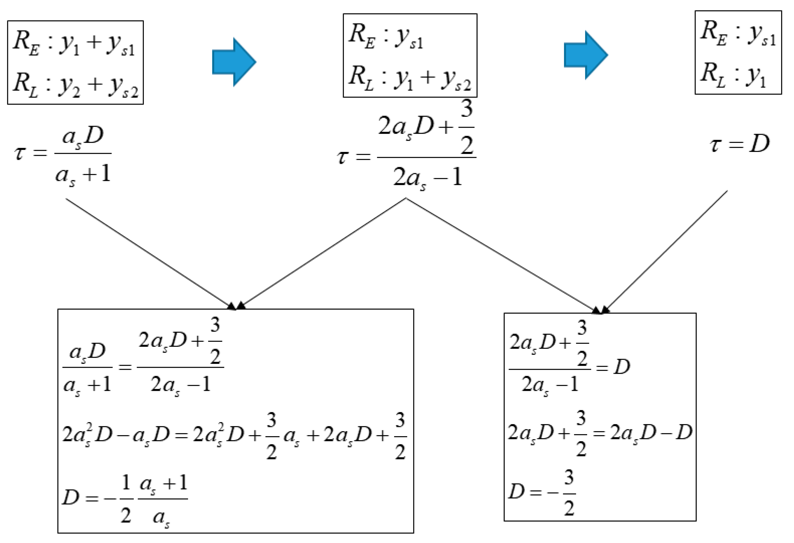
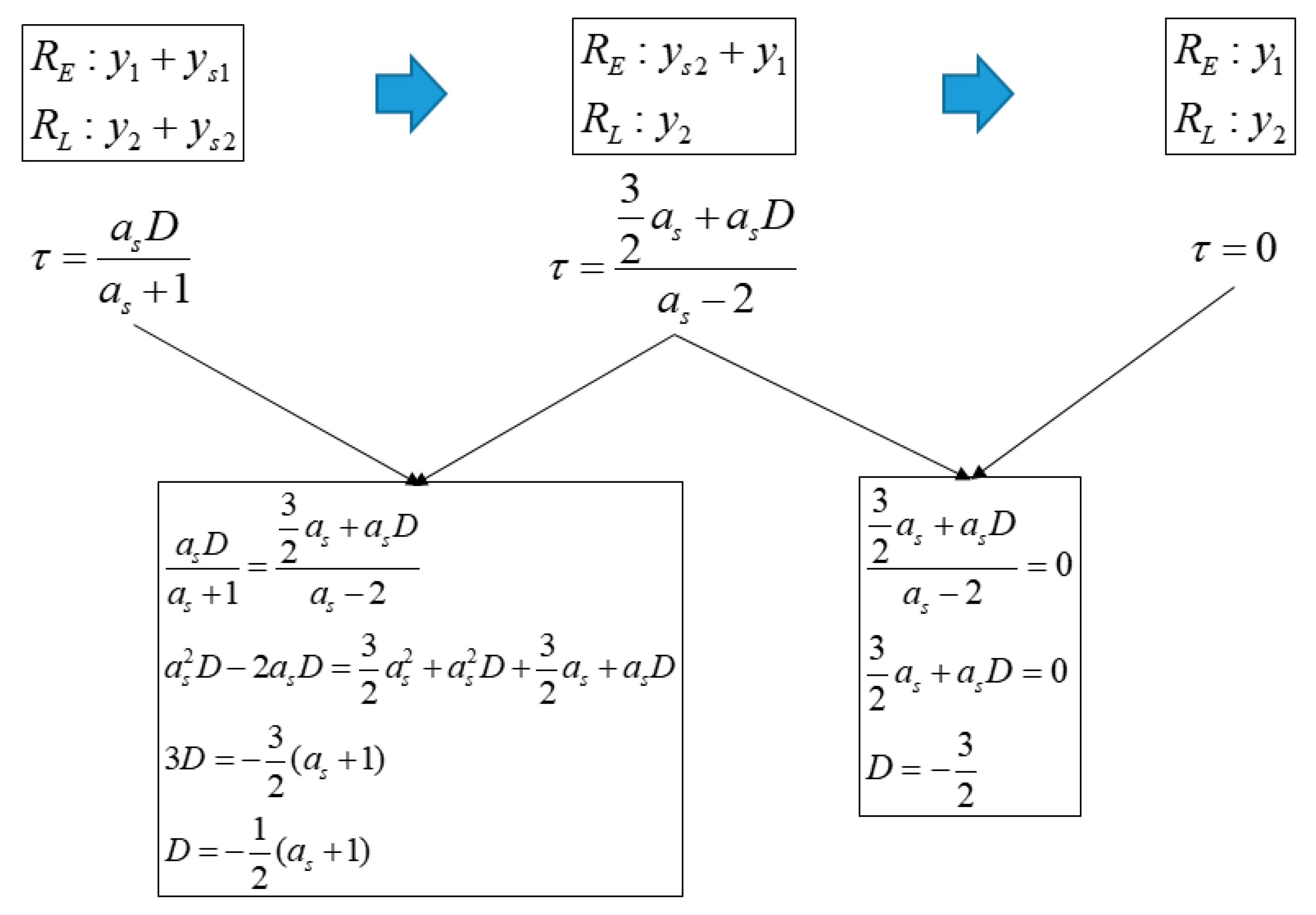
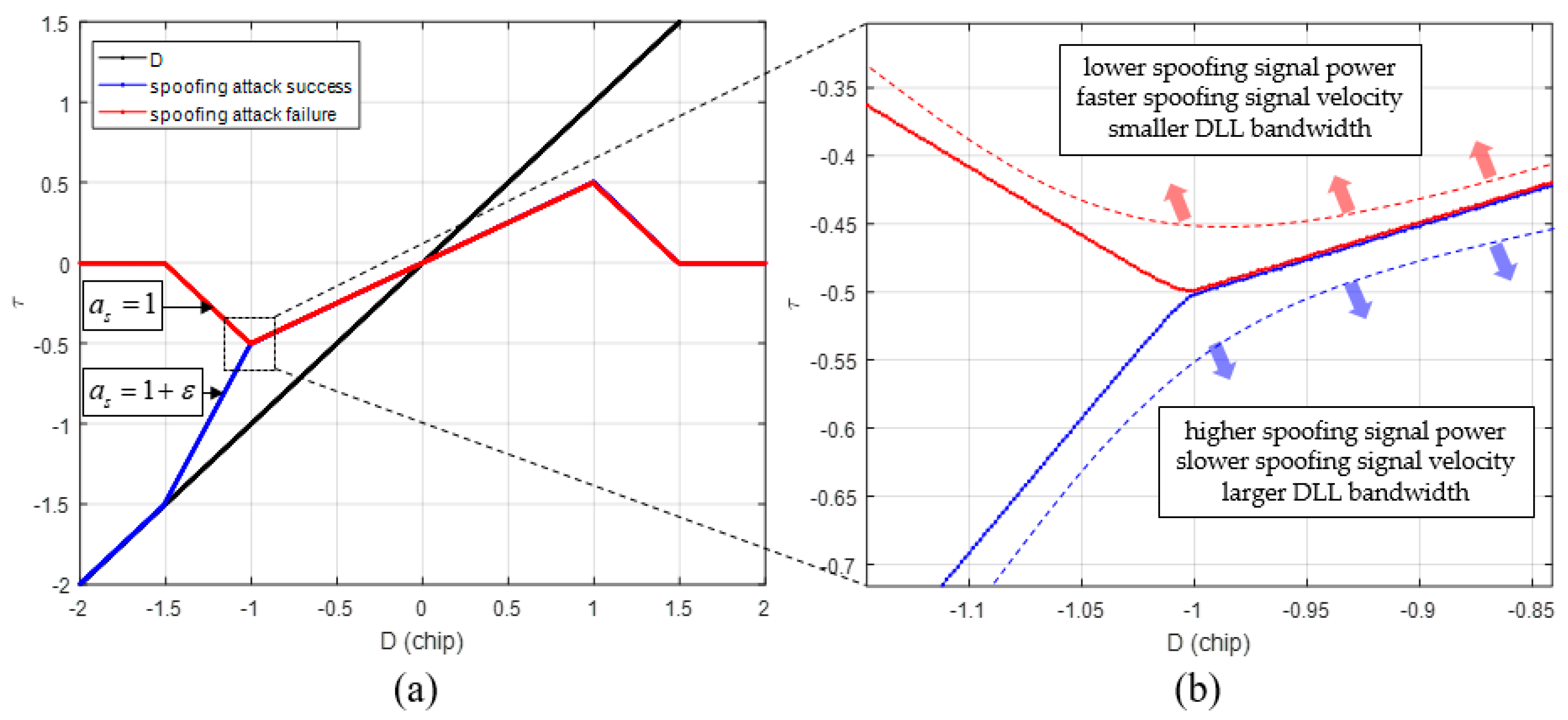
4.2. Proposed Approach for τ Calculation
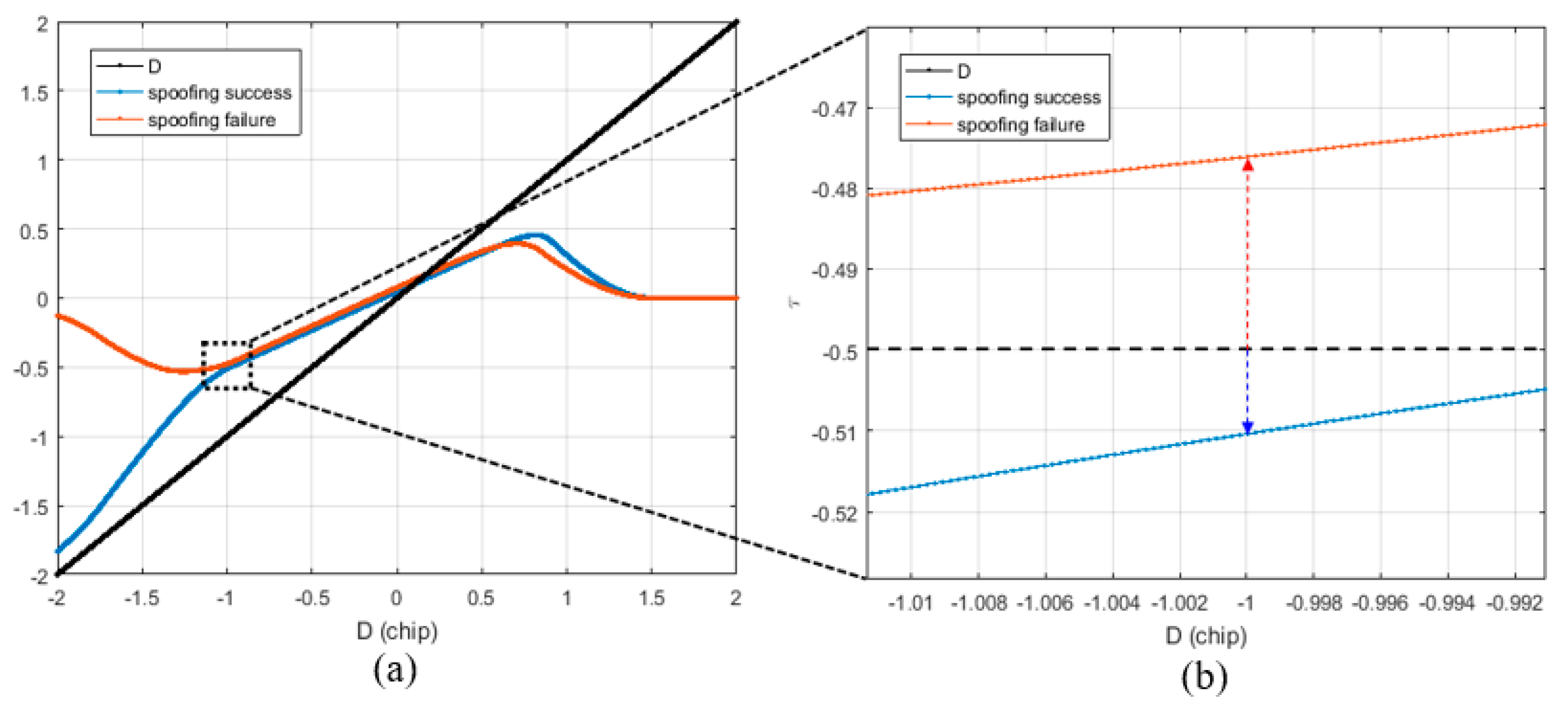
4.3. Spoofing Attack Success or Failure Criteria
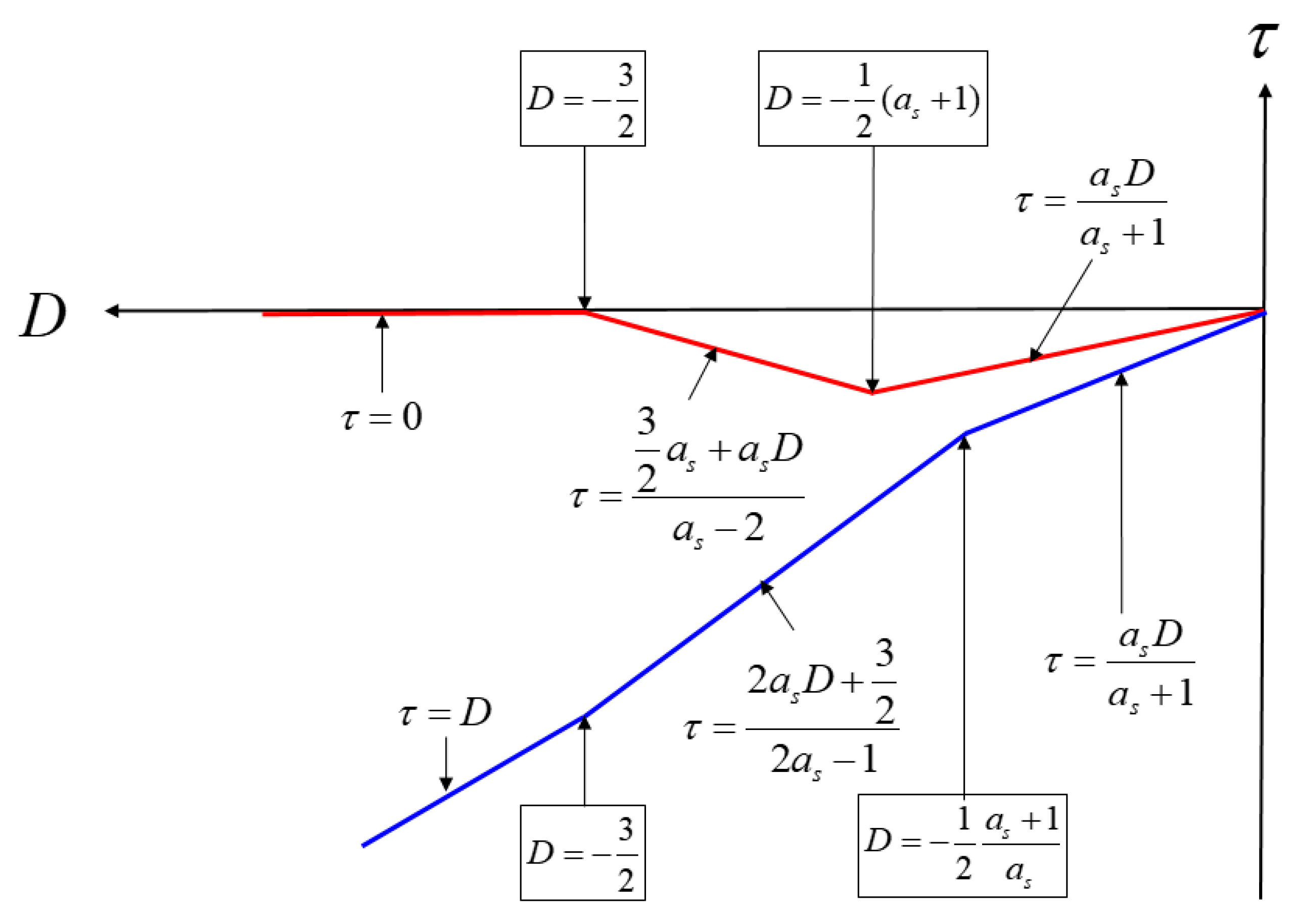
4.4. Derivation of SPE
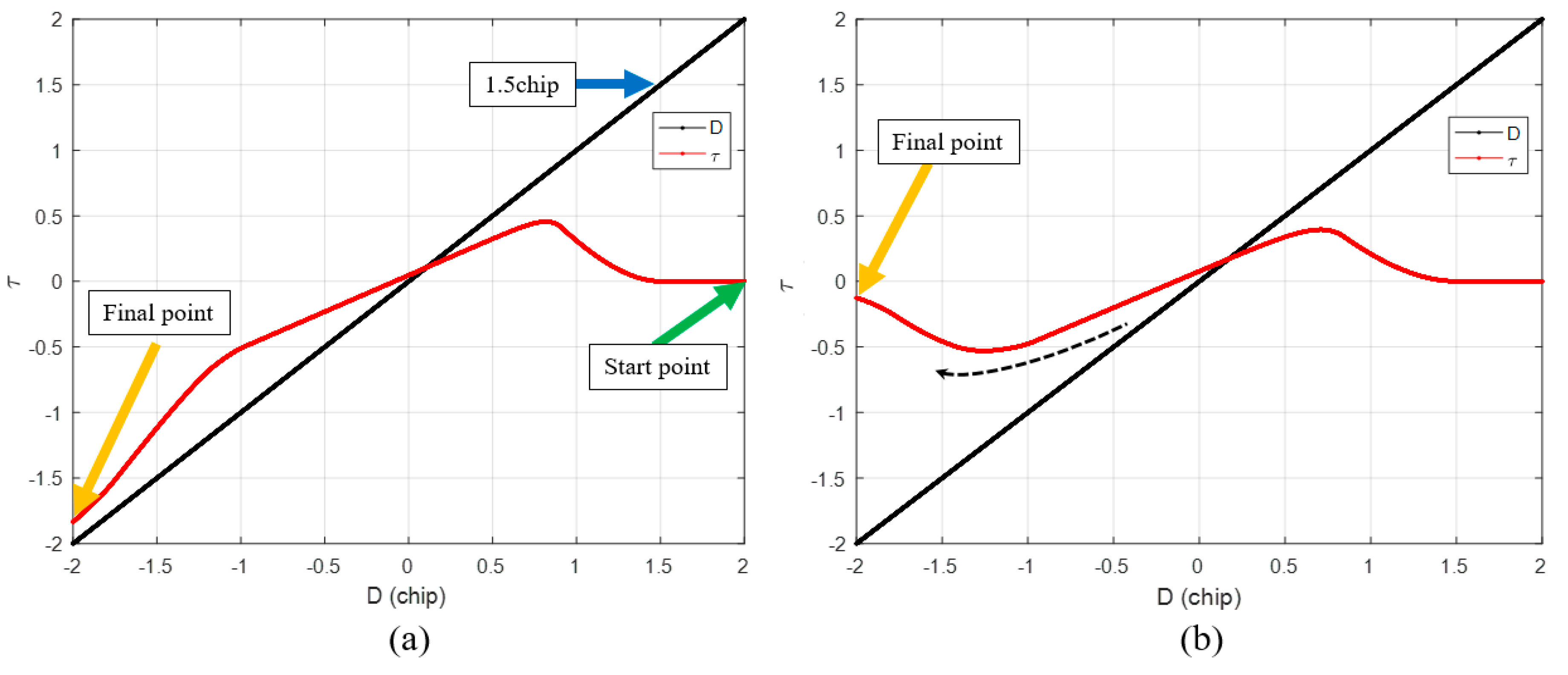
5. Analysis of SPE Simulation Results
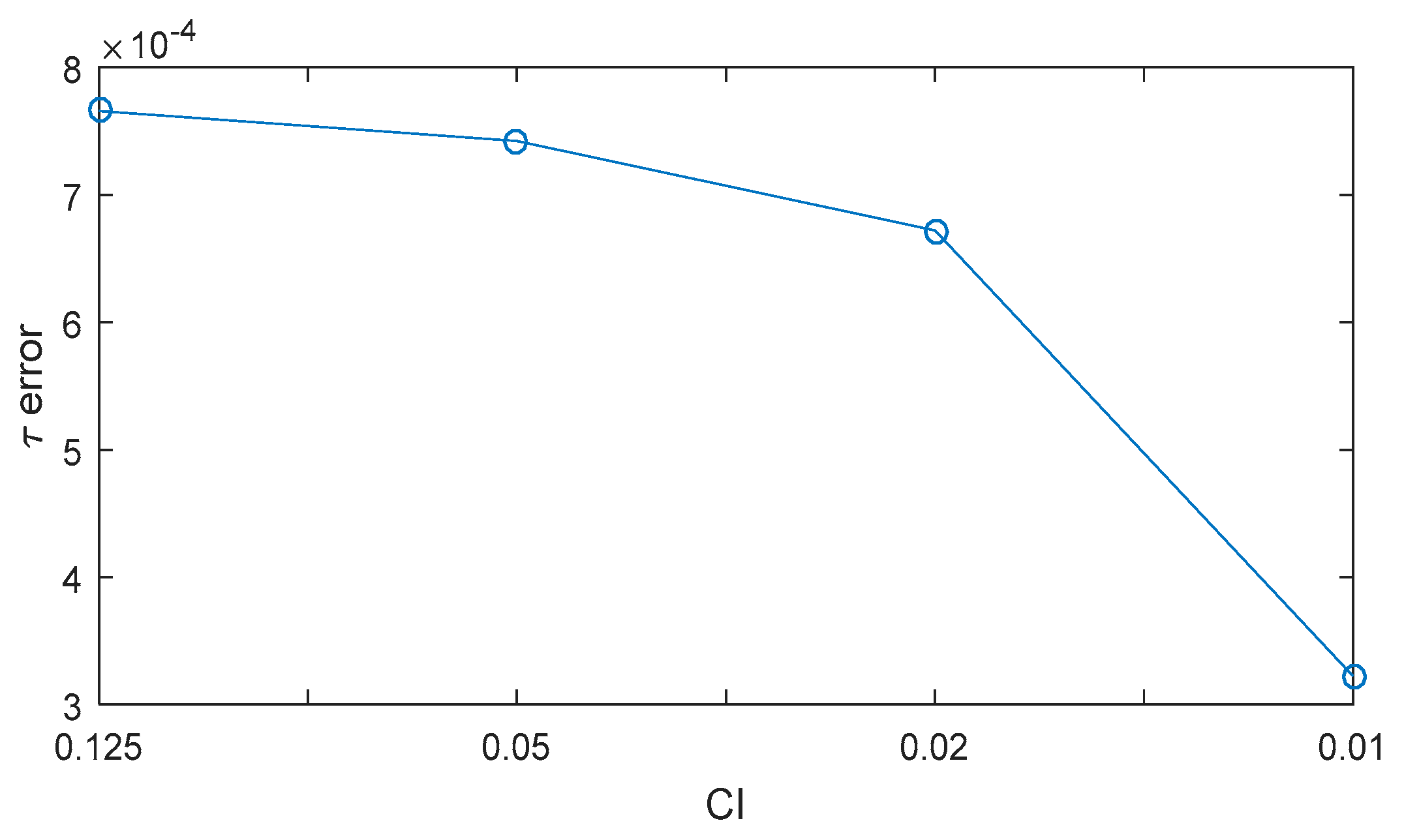
5.1. SPE Performance Analysis
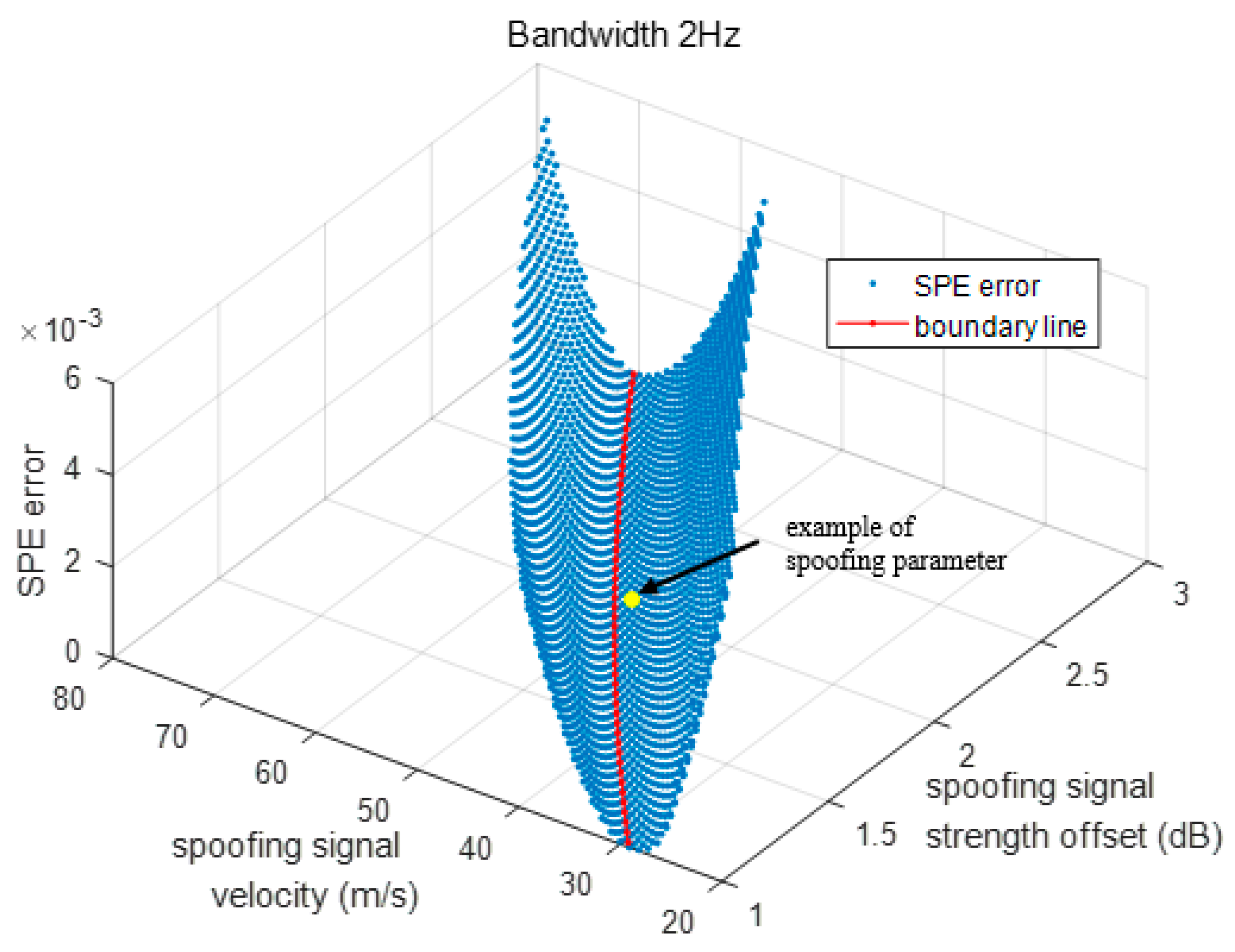
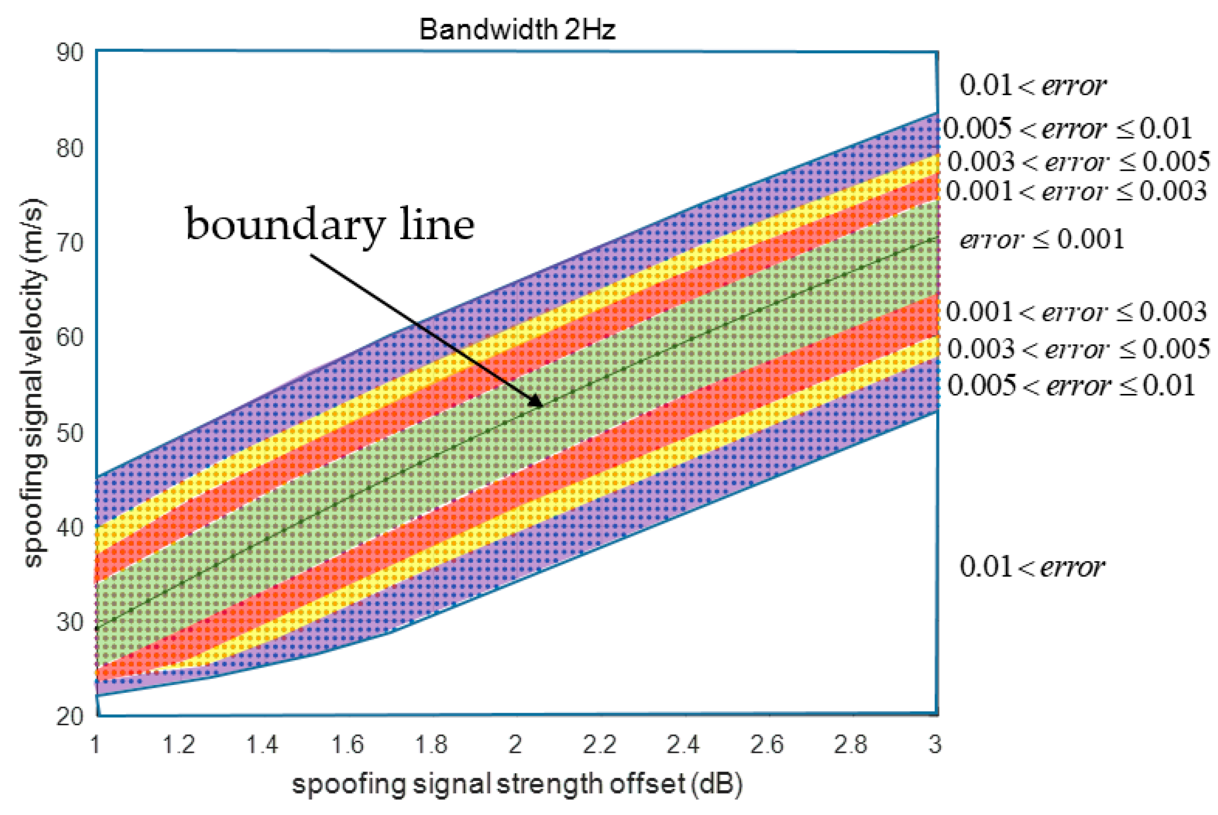
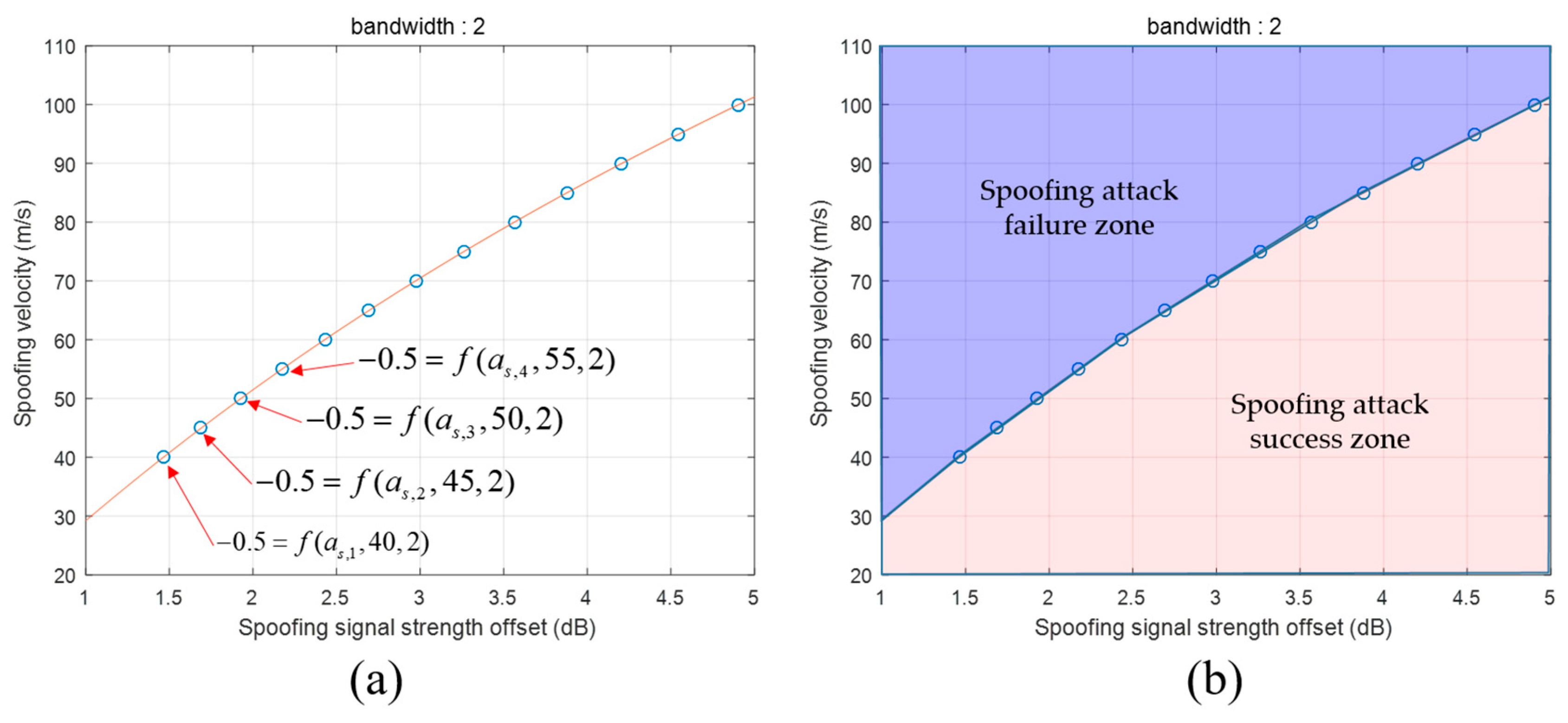
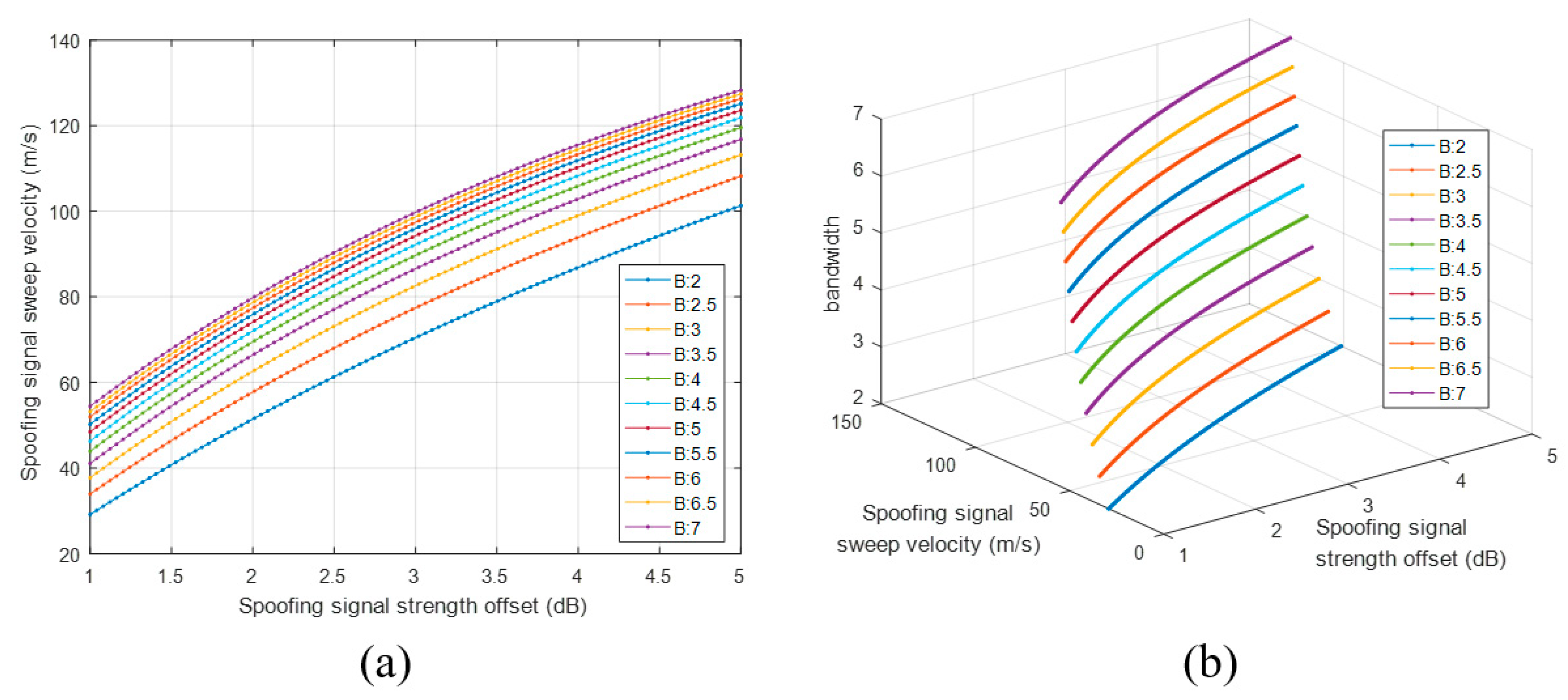
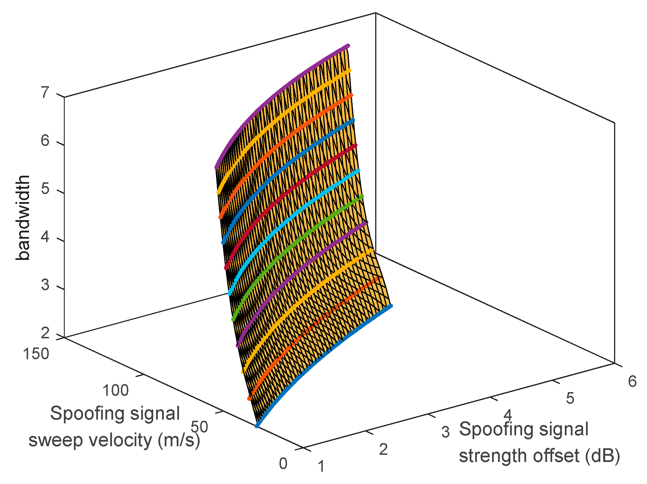
5.2. Determination of Boundary Line and Surface Using SPE
6. Discussion
- The SPE can be derived in the same manner regardless of the DLL order. The details of the same are given in Appendix B.
- In this paper, we analyzed the effect of the spoofing signal on the local replica code phase using the SPE. However, for a completely successful spoofing attack, the point of FLL tracking should be moved from the authentic signal to the spoofing signal. In the future, we will focus on spoofing process analysis in the frequency domain.
- Our simulation is conducted without any noise. If noise is added to our simulation, the probability distribution around the boundary line can be obtained using the SPE. The probability of spoofing attack success or failure on the boundary line would be 50%.
7. Conclusions
Author Contributions
Acknowledgments
Conflicts of Interest
Appendix A

Appendix B
References
- Psiaki, M.L.; Humphreys, T.E. GNSS Spoofing and Detection. Proc. IEEE 2016, 104, 1258–1270. [Google Scholar] [CrossRef]
- Cavaleri, A.; Motella, B.; Pini, M.; Fantino, M. Detection of spoofed GPS signals at code and carrier tracking level. In Proceedings of the 2010 5th ESA Workshop on Satellite Navigation Technologies and European Workshop on GNSS Signals and Signal Processing (NAVITEC), Noordwijk, The Netherlands, 8–10 December 2010; pp. 1–6. [Google Scholar]
- Tippenhauer, N.O.; Pöpper, C.; Rasmussen, K.B.; Capkun, S. On the requirements for successful GPS spoofing attacks. In Proceedings of the 18th ACM Conference on Computer and Communications Security, Chicago, IL, USA, 17–21 October 2011. [Google Scholar] [CrossRef]
- Hui, H.; Na, W. A study of GPS jamming and anti-jamming. In Proceedings of the 2009 2nd International Conference on Power Electronics and Intelligent Transportation System (PEITS), Shenzhen, China, 19–20 December 2009. [Google Scholar] [CrossRef]
- Ng, Y.; Gao, G.X. Mitigating jamming and meaconing attacks using direct GPS positioning. In Proceedings of the 2016 IEEE/ION Position, Location and Navigation Symposium (PLANS), Savannah, GA, USA, 11–14 April 2016; pp. 1021–1026. [Google Scholar] [CrossRef]
- Kerns, A.J.; Shepard, D.P.; Bhatti, J.A.; Humphreys, T.E. Unmanned aircraft capture and control via GPS spoofing. J. Field Robot. 2014, 31, 617–636. [Google Scholar] [CrossRef]
- Jafarnia-Jahromi, A.; Broumandan, A.; Nielsen, J.; Lachapelle, G. GPS vulnerability to spoofing threats and a review of antispoofing techniques. Int. J. Navig. Obs. 2012, 2012. [Google Scholar] [CrossRef]
- Humphreys, T.E.; Ledvina, B.M.; Tech, V.; Psiaki, M.L.; Hanlon, B.W.O.; Kintner, P.M. Assessing the Spoofing Threat: Development of a Portable GPS Civilian Spoofer. In Proceedings of the 21st International Technical Meeting of the Satellite Division of The Institute of Navigation (ION GNSS 2008), Savannah, GA, USA, 16–19 September 2008; pp. 2314–2325. [Google Scholar] [CrossRef]
- Shepard, D.P.; Bhatti, J.A.; Humphreys, T.E. Drone Hack: Spoofing Attack Demonstration on a Civilian Unmanned Aerial Vehicle. GPS World 2012, 23, 30–33. [Google Scholar]
- Bhatti, J.; Humphreys, T.E. Hostile Control of Ships via False GPS Signals: Demonstration and Detection. Navig. J. Inst. Navig. 2017, 64, 51–66. [Google Scholar] [CrossRef]
- Wang, K.; Chen, S.; Pan, A. Time and Position Spoofing with Open Source Projects; Black Hat: London, UK, 2015; p. 148. [Google Scholar]
- Wang, F.; Li, H.; Lu, M. GNSS spoofing detection and mitigation based on maximum likelihood estimation. Sensors 2017, 17, 1532. [Google Scholar] [CrossRef] [PubMed]
- Psiaki, M.L.; O’Hanlon, B.W.; Bhatti, J.A.; Shepard, D.P.; Humphreys, T.E. GPS spoofing detection via dual-receiver correlation of military signals. IEEE Trans. Aerosp. Electron. Syst. 2013, 49, 2250–2267. [Google Scholar] [CrossRef]
- Manfredini, E.G.; Dovis, F. On the use of a feedback tracking architecture for satellite navigation spoofing detection. Sensors 2016, 16, 2051. [Google Scholar] [CrossRef] [PubMed]
- Liu, K.; Wu, W.; Wu, Z.; He, L.; Tang, K. Spoofing detection algorithm based on pseudorange differences. Sensors 2018, 18, 3197. [Google Scholar] [CrossRef] [PubMed]
- Shafiee, E.; Mosavi, M.R.; Moazedi, M. Detection of Spoofing Attack using Machine Learning based on Multi-Layer Neural Network in Single-Frequency GPS Receivers. J. Navig. 2018, 71, 169–188. [Google Scholar] [CrossRef]
- Daneshmand, S.; Jafarnia-jahromi, A.; Broumandan, A.; Lachapelle, G. A Low-Complexity GPS Anti-Spoofing Method Using a Multi-Antenna Array. In Proceedings of the 25th International Technical Meeting of The Satellite Division of the Institute of Navigation, Nashville, TN, USA, 17–21 September 2012. [Google Scholar]
- Broumandan, A.; Lachapelle, G. Spoofing Detection Using GNSS/INS/Odometer Coupling for Vehicular Navigation. Sensors 2018, 18, 1305. [Google Scholar] [CrossRef] [PubMed]
- Perdue, L.; Sasaki, H.; Fischer, J. Testing GNSS Receivers to Harden Against Spoofing Attacks. In Proceedings of the International Symposium on GNSS 2015, Kyoto, Japan, 16–19 November 2015. [Google Scholar]
- Ma, C.; Lachapelle, G.; Cannon, M.E. Implementation of a Software GPS Receiver. Architecture 2003, 2004, 956–970. [Google Scholar]


| Parameters | Spoofing Attack Success Probability |
|---|---|
| Increase in the spoofing signal strength | Increase |
| Increase in spoofing signal sweep velocity | Decrease |
| Increase in the DLL bandwidth | Increase |
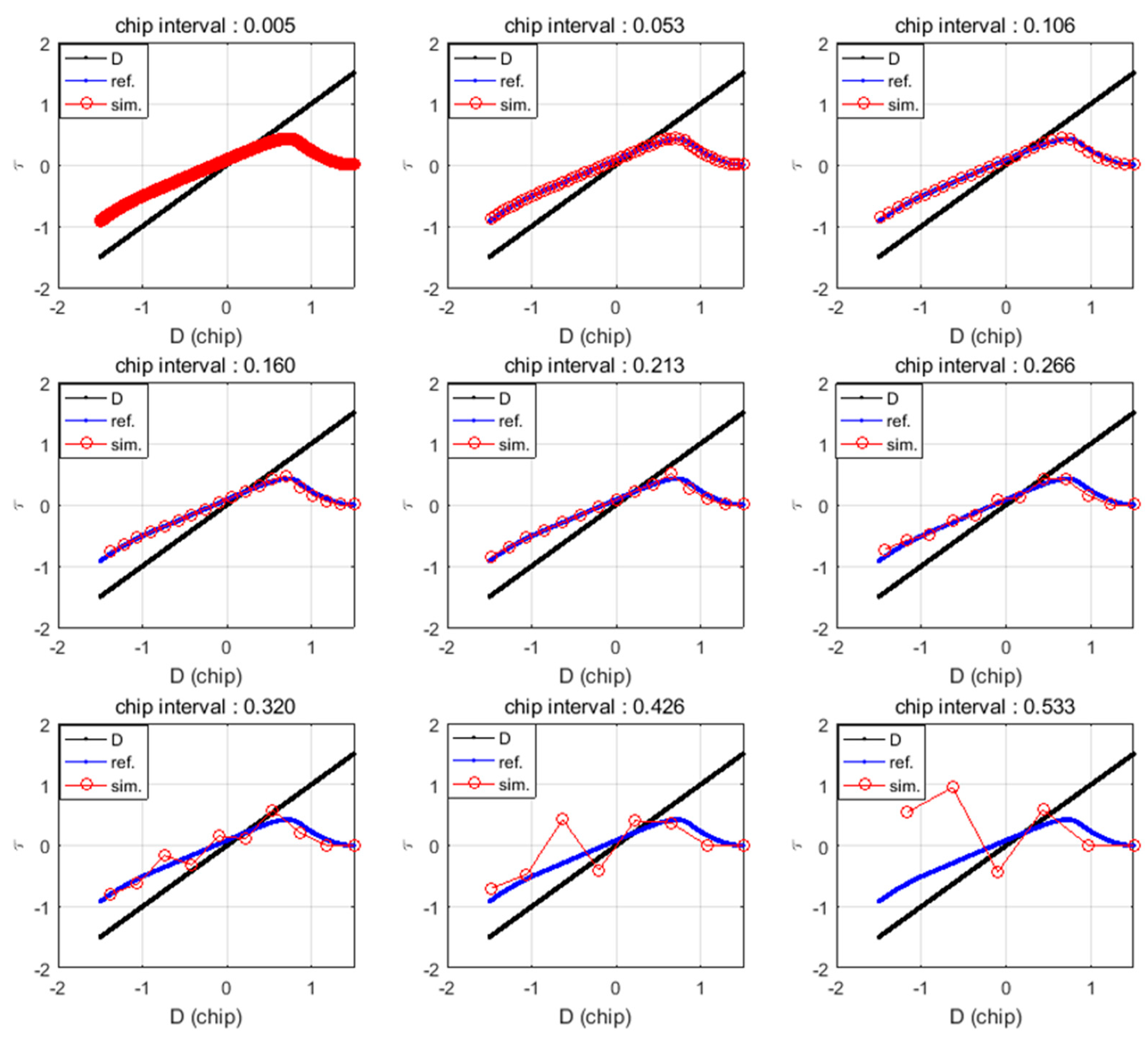
| Chip Interval (chip) | Time Interval (second) |
|---|---|
| 0.005 | 0.0183 |
| 0.053 | 0.1941 |
| 0.125 | 0.4578 |
| 0.160 | 0.5860 |
| 0.213 | 0.7801 |
| 0.266 | 0.9742 |
| 0.320 | 1.1720 |
| 0.426 | 1.5602 |
| 0.533 | 1.9521 |
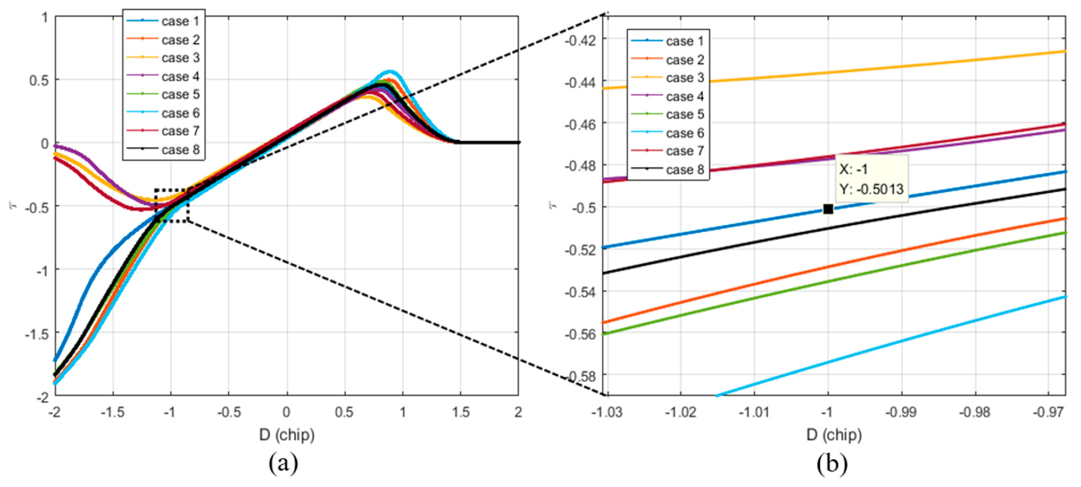
| Case | Spoofing Signal Strength Offset (dB) | Sweep Velocity (m/s) | Bandwidth | Spoofing Results | at D = −1 |
|---|---|---|---|---|---|
| 1 | 1.5 | 50 | 3 | Success | 0.5013 |
| 2 | 1.5 | 50 | 5 | Success | 0.5287 |
| 3 | 1.5 | 70 | 3 | Failure | 0.4362 |
| 4 | 1.5 | 70 | 5 | Failure | 0.4774 |
| 5 | 2 | 50 | 3 | Success | 0.5357 |
| 6 | 2 | 50 | 5 | Success | 0.5741 |
| 7 | 2 | 70 | 3 | Failure | 0.4761 |
| 8 | 2 | 70 | 5 | Success | 0.5104 |
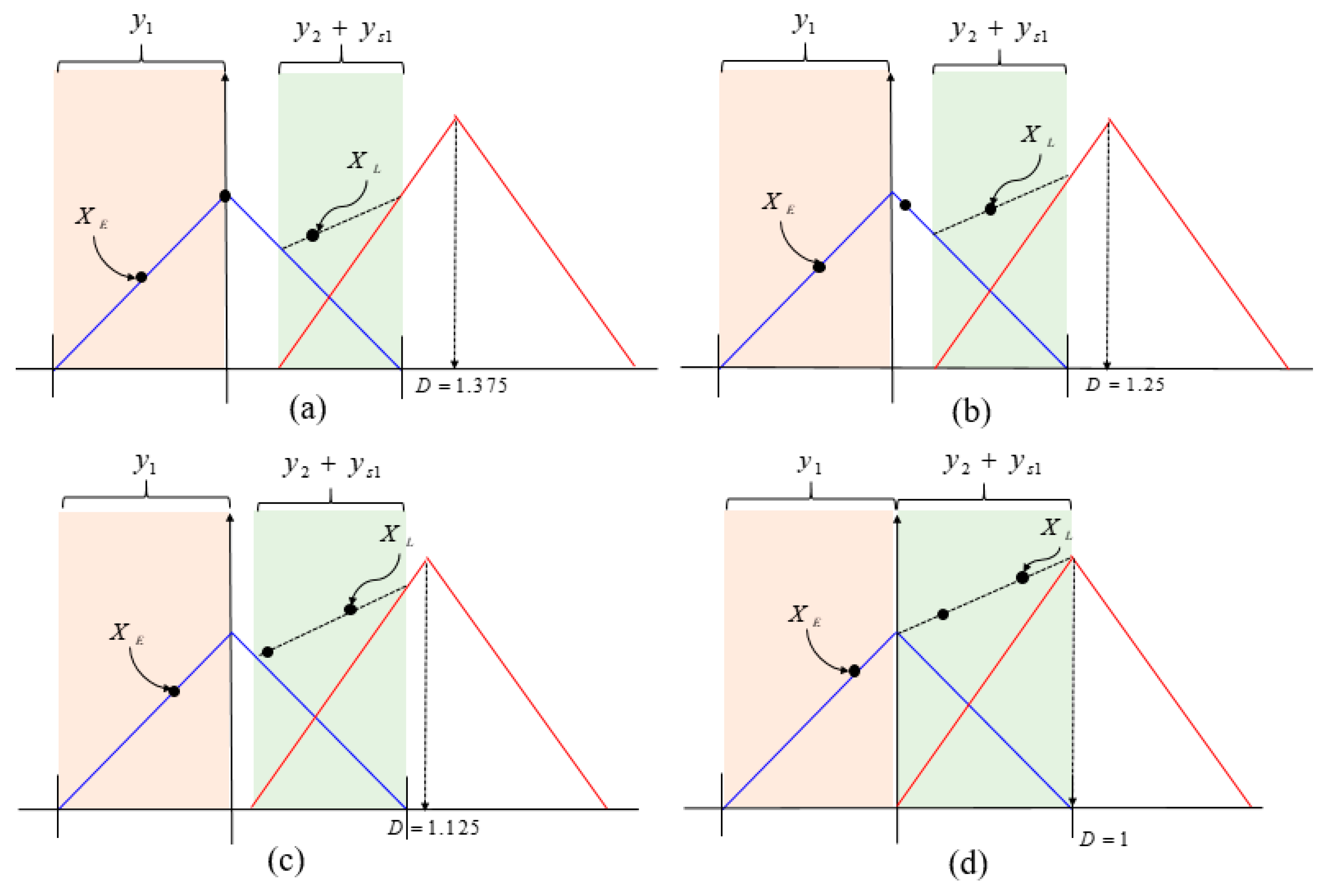
| i | D[i] | Range of | Range of | ACF model of XE | ACF model of XL |
|---|---|---|---|---|---|
| 1 | 1.375 | −1~0 | 0.375~1 | y1 | y2 + ys1 |
| 2 | 1.25 | −1~0 | 0.25~1 | y1 | y2 + ys1 |
| 3 | 1.125 | −1~0 | 0.125~1 | y1 | y2 + ys1 |
| 4 | 1 | −1~0 | 0~1 | y1 | y2 + ys1 |
| 5 | 0.875 | −1~−0.25 | −0.125~0.875 | y1 | y2 + ys1 |
| 6 | 0.75 | −0.25~0 | 0.75~1 | y1 + ys1 | y2 + ys2 |
| 7 | 0.675 | −0.375~0 | 0.625~1 | y1 + ys1 | y2 + ys2 |
| 8 | 0.5 | −0.5~0 | 0.5~1 | y1 + ys1 | y2 + ys2 |
| 9 | 0.375 | −0.625~0 | 0.375~1 | y1 + ys1 | y2 + ys2 |
| 10 | 0.25 | −0.75~0 | 0.25~1 | y1 + ys1 | y2 + ys2 |
| 11 | 0.125 | −0.875~0 | 0.125~1 | y1 + ys1 | y2 + ys2 |
| 12 | 0 | −1~0 | 0~1 | y1 + ys1 | y2 + ys2 |
| 13 | −0.125 | −1~−0.125 | 0~0.875 | y1 + ys1 | y2 + ys2 |
| 14 | −0.25 | −1~−0.25 | 0~0.75 | y1 + ys1 | y2 + ys2 |
| 15 | −0.375 | −1~0.375 | 0~0.625 | y1 + ys1 | y2 + ys2 |
| 16 | −0.5 | −1~−0.5 | 0~0.5 | y1 + ys1 | y2 + ys2 |
| 17 | −0.625 | −1~0.625 | 0~0.375 | y1 + ys1 | y2 + ys2 |
| 18 | −0.75 | −1~−0.75 | 0~0.25 | y1 + ys1 | y2 + ys2 |
| 19 | −0.875 | −1~0.875 | 0~0.125 | y1 + ys1 | y2 + ys2 |
| Case | Spoofing Signal Strength Offset (dB) | Sweep Velocity (m/s) | Bandwidth | Reference | Proposed | Error |
|---|---|---|---|---|---|---|
| 1 | 1.5 | 55 | 3 | −0.4895 | −0.4903 | 0.0008 |
| 2 | 1.5 | 60 | 3 | −0.4742 | −0.4777 | 0.0035 |
| 3 | 1.5 | 60 | 5 | −0.5043 | −0.503 | 0.0013 |
| 4 | 1.5 | 65 | 5 | −0.4927 | −0.4931 | 0.0004 |
| 5 | 2 | 60 | 3 | −0.5072 | −0.507 | 0.0002 |
| 6 | 2 | 65 | 3 | −0.4934 | −0.4937 | 0.0003 |
| 7 | 2 | 65 | 5 | −0.5257 | −0.5217 | 0.004 |
| 8 | 2 | 70 | 3 | −0.477 | −0.4797 | 0.0027 |
| 9 | 2 | 70 | 5 | −0.5112 | −0.5104 | 0.0008 |
| 10 | 2.5 | 65 | 3 | −0.5253 | −0.5231 | 0.0022 |
| 11 | 2.5 | 80 | 3 | −0.4759 | −0.4787 | 0.0028 |
| 12 | 2.5 | 80 | 5 | −0.5147 | −0.5136 | 0.0011 |
| Number | Sweep Velocity (m/s) | Bandwidth (Hz) | (Hz) |
|---|---|---|---|
| 1 | 40 | 2 | 1.46 |
| 2 | 45 | 2 | 1.69 |
| 3 | 50 | 2 | 1.92 |
| 4 | 55 | 2 | 2.17 |
| 5 | 60 | 2 | 2.42 |
| 6 | 65 | 2 | 2.69 |
| 7 | 70 | 2 | 2.97 |
| 8 | 75 | 2 | 3.26 |
| 9 | 80 | 2 | 3.56 |
| 10 | 85 | 2 | 3.87 |
| 11 | 90 | 2 | 4.20 |
| 12 | 95 | 2 | 4.54 |
| 13 | 100 | 2 | 4.09 |
| Sweep Velocity (m/s) | Conventional DLL | SPE | ||
|---|---|---|---|---|
| The Number of Iteration | Computational Time (s) | The Number of Iteration | Computational Time (s) | |
| 40 | 18312 | 10.34 | 19 | 0.24 |
| 50 | 14650 | 8.26 | 19 | 0.24 |
| 60 | 12208 | 6.86 | 19 | 0.24 |
| 70 | 10464 | 5.89 | 19 | 0.24 |
| 80 | 9156 | 5.17 | 19 | 0.24 |
© 2019 by the authors. Licensee MDPI, Basel, Switzerland. This article is an open access article distributed under the terms and conditions of the Creative Commons Attribution (CC BY) license (http://creativecommons.org/licenses/by/4.0/).
Share and Cite
Shin, B.; Park, M.; Jeon, S.; So, H.; Kim, G.; Kee, C. Spoofing Attack Results Determination in Code Domain Using a Spoofing Process Equation. Sensors 2019, 19, 293. https://doi.org/10.3390/s19020293
Shin B, Park M, Jeon S, So H, Kim G, Kee C. Spoofing Attack Results Determination in Code Domain Using a Spoofing Process Equation. Sensors. 2019; 19(2):293. https://doi.org/10.3390/s19020293
Chicago/Turabian StyleShin, Beomju, Minhuck Park, Sanghoon Jeon, Hyoungmin So, Gapjin Kim, and Changdon Kee. 2019. "Spoofing Attack Results Determination in Code Domain Using a Spoofing Process Equation" Sensors 19, no. 2: 293. https://doi.org/10.3390/s19020293
APA StyleShin, B., Park, M., Jeon, S., So, H., Kim, G., & Kee, C. (2019). Spoofing Attack Results Determination in Code Domain Using a Spoofing Process Equation. Sensors, 19(2), 293. https://doi.org/10.3390/s19020293