An On-Orbit Dynamic Calibration Method for an MHD Micro-Angular Vibration Sensor Using a Laser Interferometer

Abstract
:1. Introduction
1.1. Background
1.2. Methodology
2. Methods and Principle
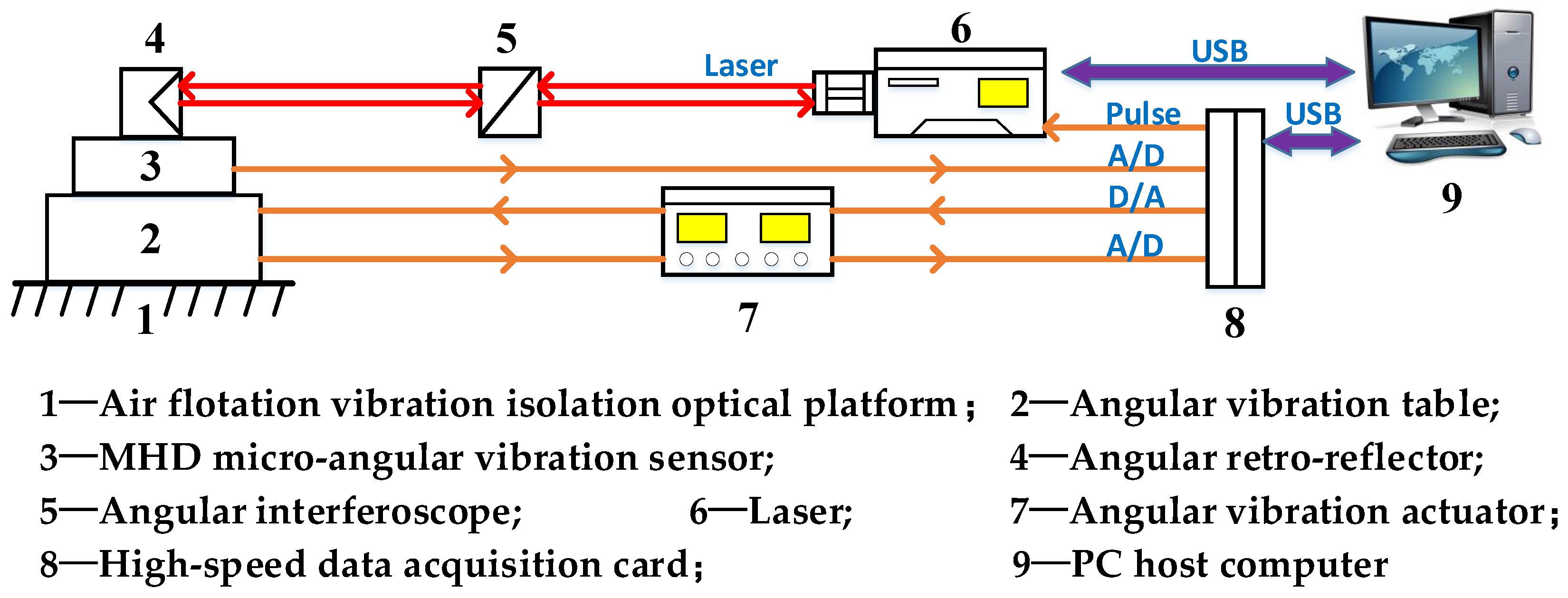
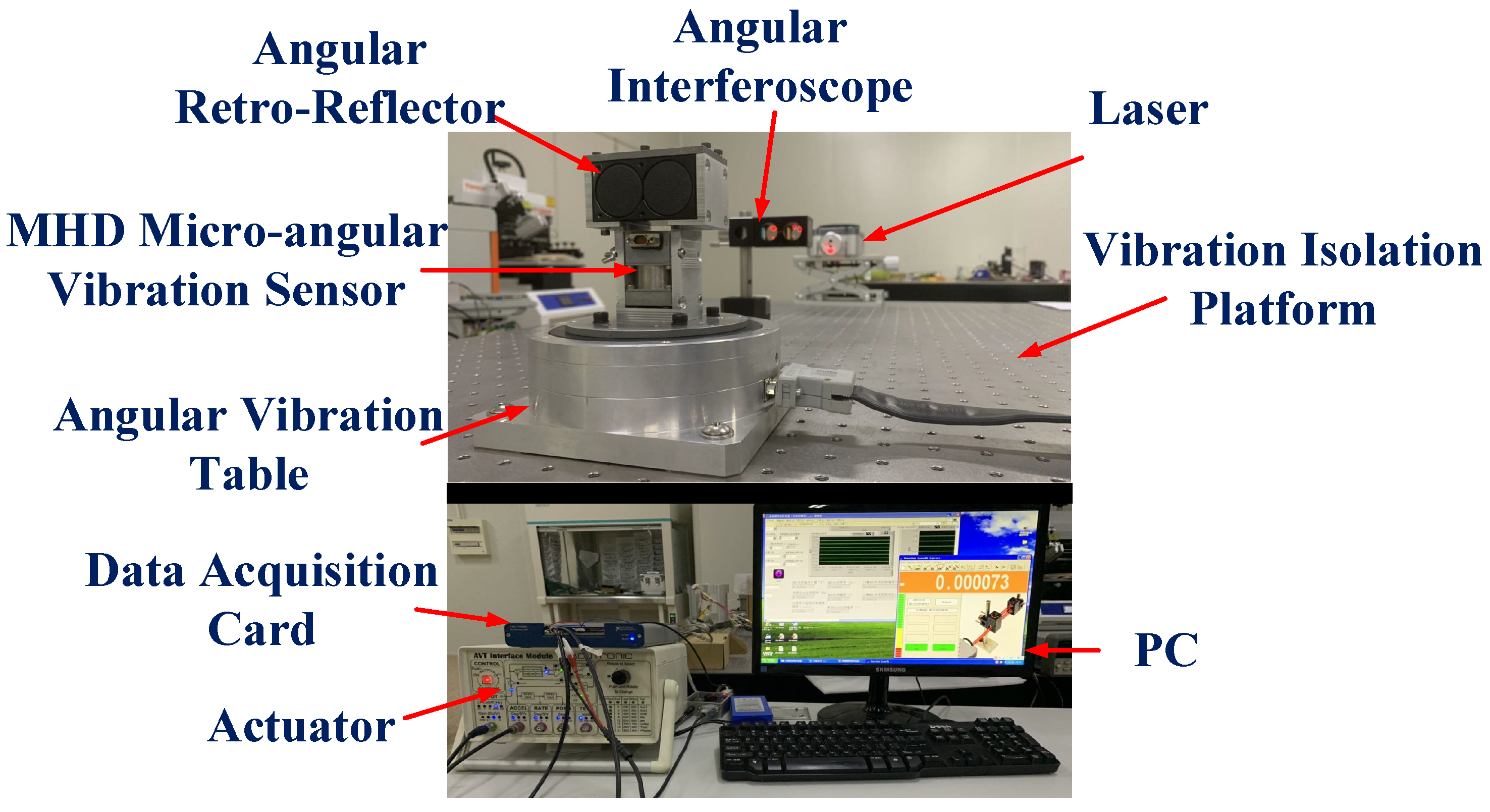
2.1. System Configuration
2.2. Theoretical Background
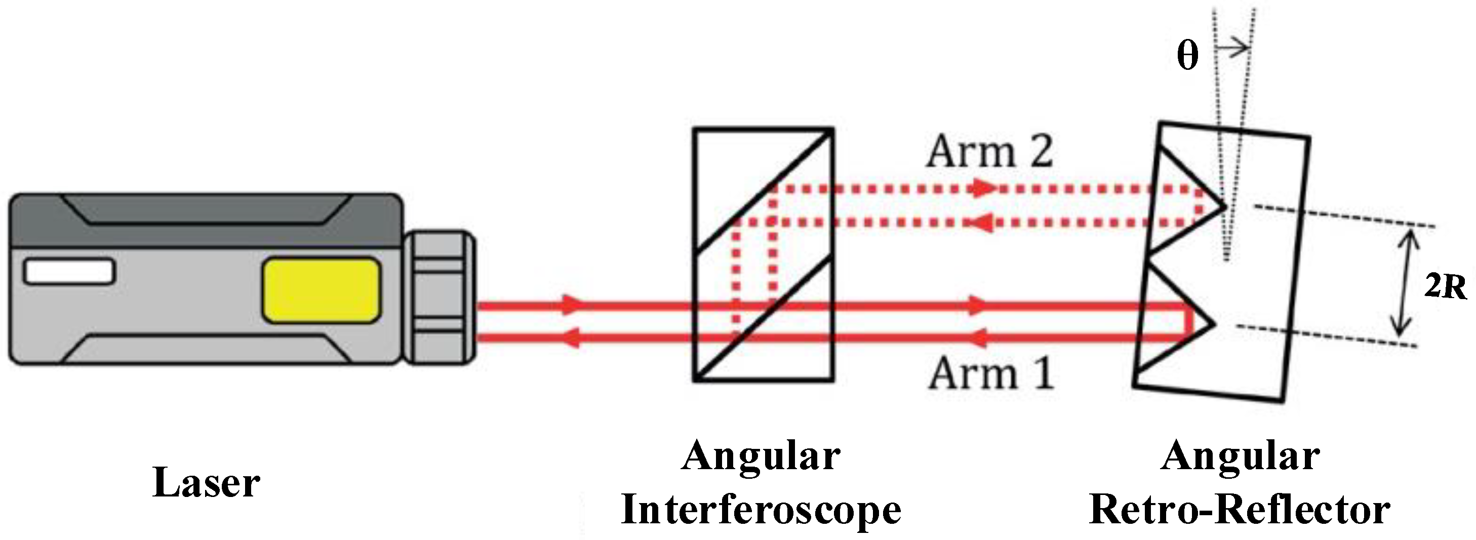
2.2.1. Michelson Laser Interference Principle and the Sinusoidal Approximation Method
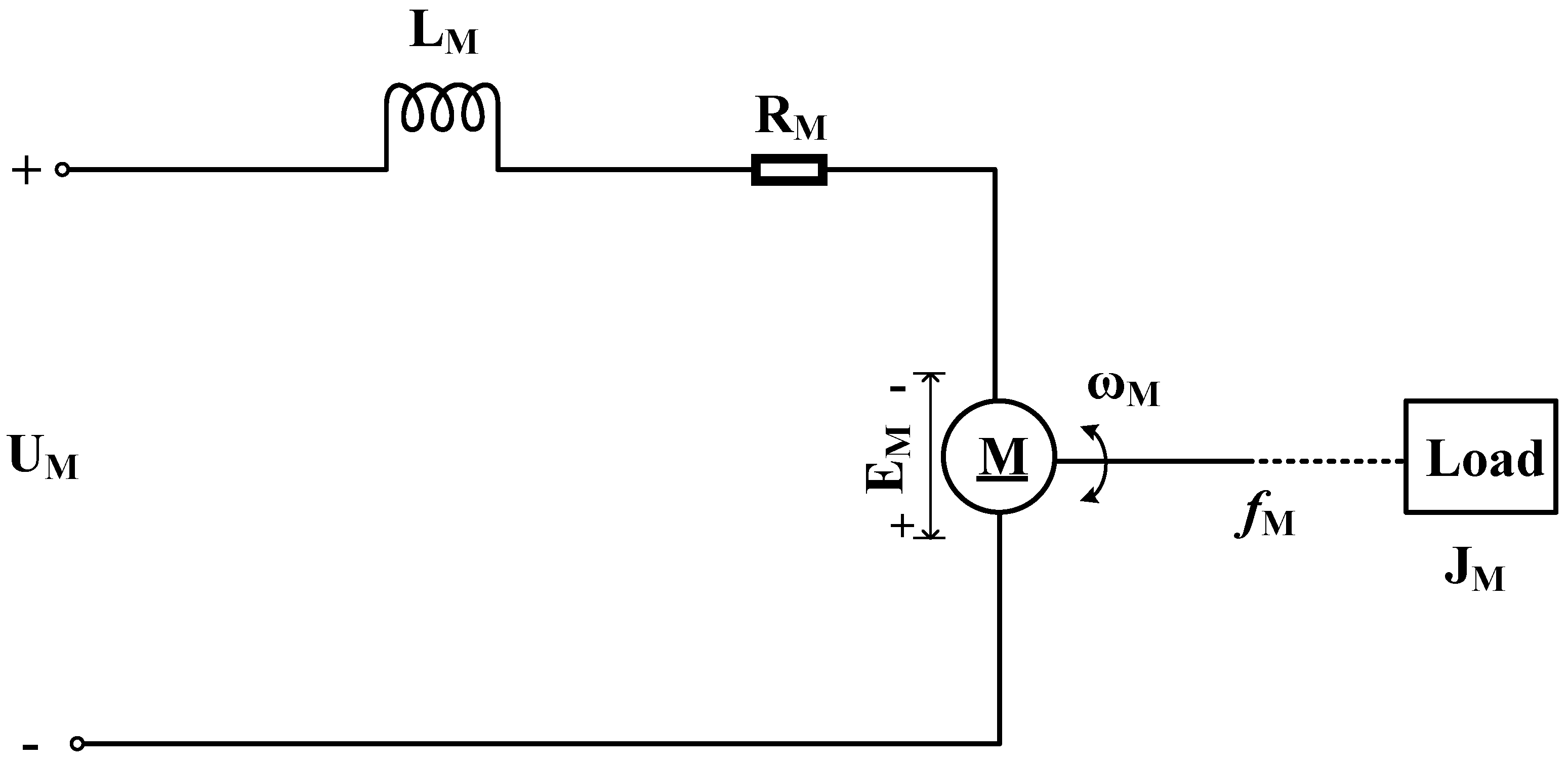
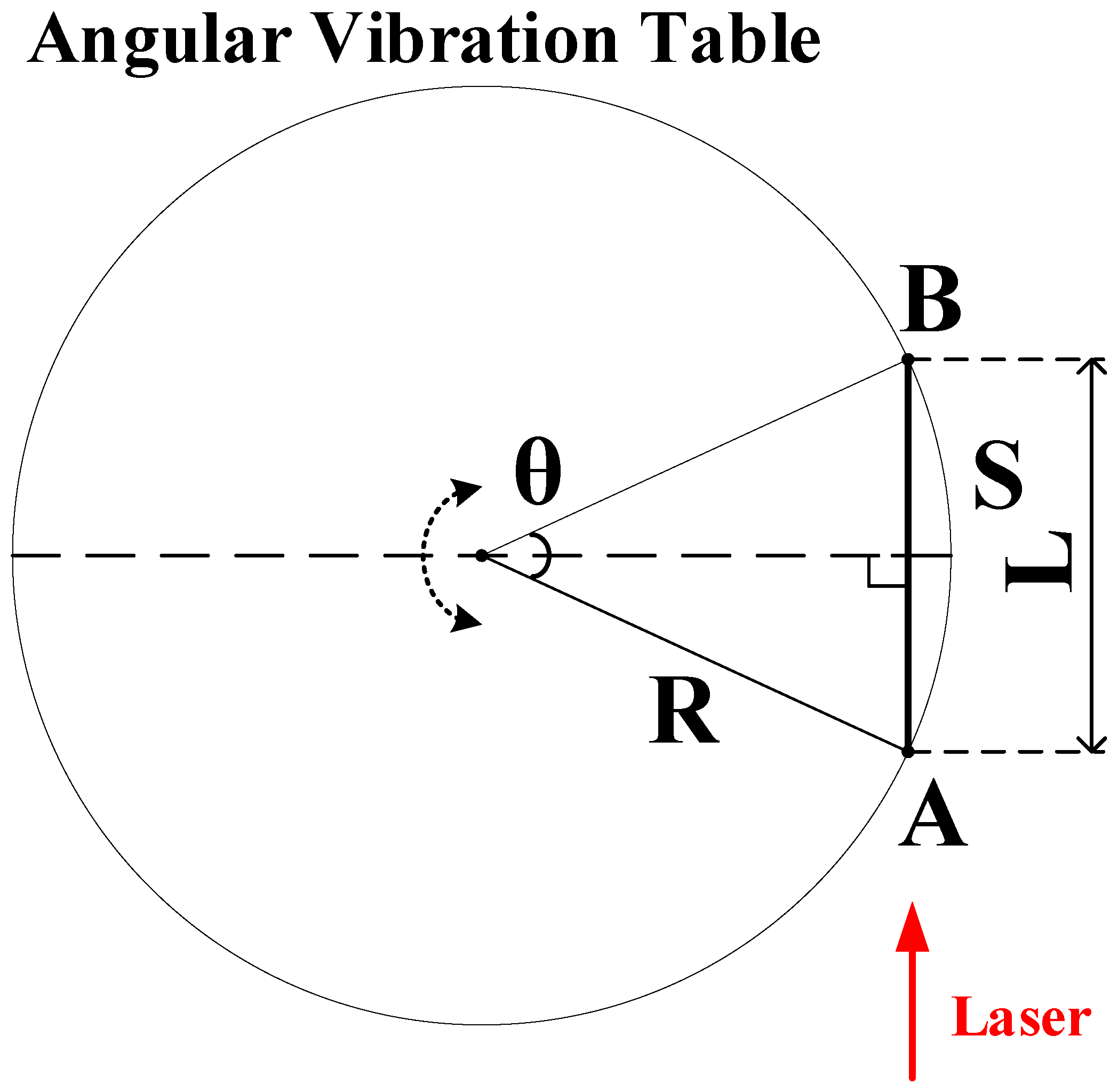
2.2.2. Principle of the Angular Vibration Excitation System
2.3. System Error
2.3.1. Principle Error
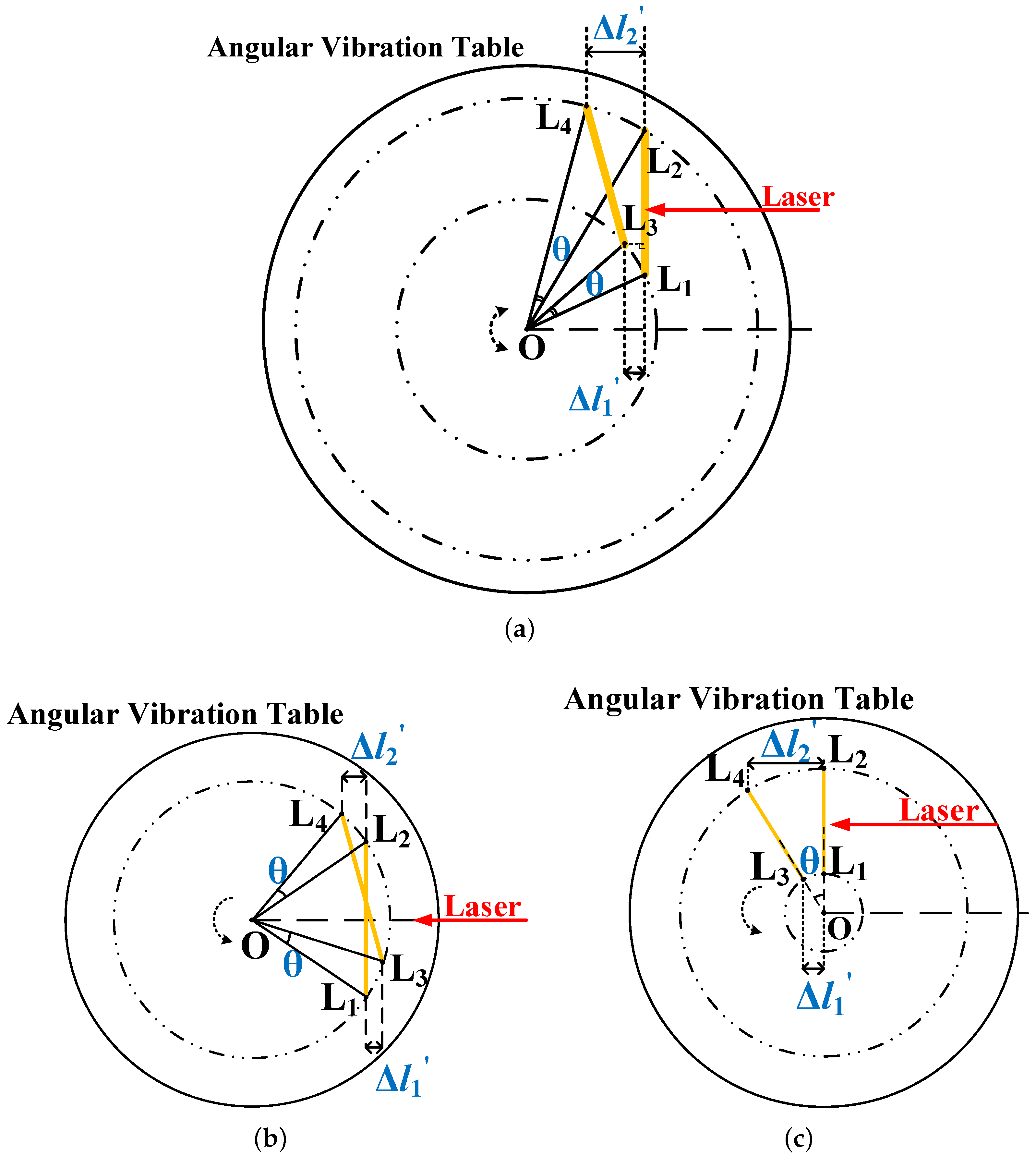
2.3.2. The Eccentric Installation Error of the Angular Retroreflector
- When the angular retroreflector is completely located in the first quadrant, the measuring retardation can be represented as .If , mm, and are assumed, then mm.Then, the relative angular error induced by eccentricity is .
- When the angular retroreflector is translated a distance from the center position in the opposite direction of the optical path incidence, the measured optical path difference can be expressed as .
- When the angular retroreflector is translated from the center position by a distance along the vertical direction of the optical path and is above point O, the measured optical path difference can be expressed as .
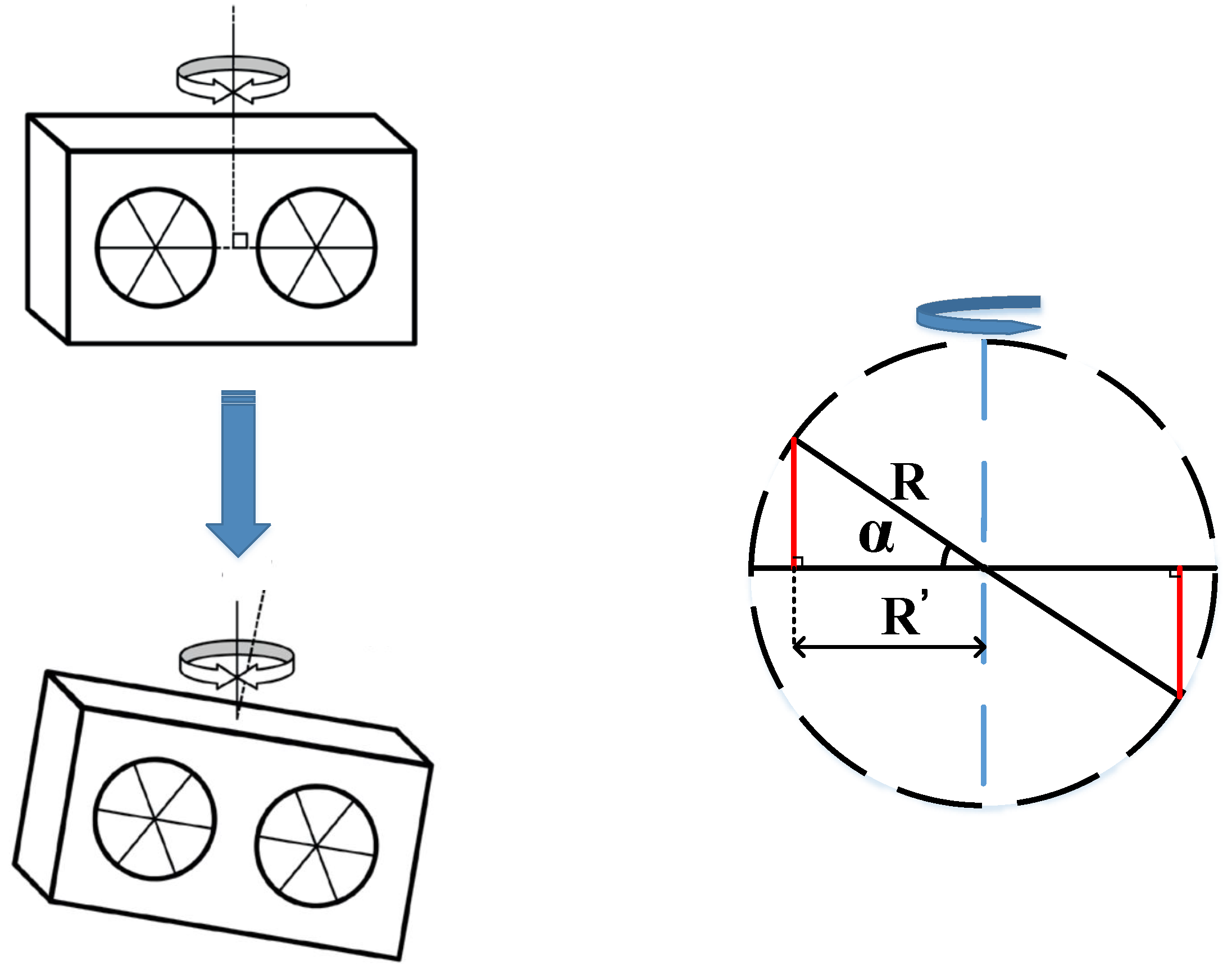
2.3.3. The Tilt Installation Error of the Angular Retroreflector
2.3.4. The Tilt Installation Error of the Optical path
3. Results
3.1. Experimental Setup
3.2. Experimental Results
3.2.1. Frequency Response and Distortion of the Excitation System Carrying Different Loads
3.2.2. Performance Experiments for the Homodyne Laser Interferometric Calibration System
3.2.3. Complex Sensitivity Calibration Experiments of the MHD Micro-Angular Vibration Sensor
3.2.4. Uncertainty Evaluation of the System
4. Conclusions
- The evaluated amplitude uncertainty is much less than the international standard of , while the phase shift uncertainty is larger than . This is possibly caused by the complex vibration mode of the mechanical structure for small-amplitude and high-frequency vibration. Although the mechanical clamp was designed to reduce the barycenter and increase the structural stiffness to the greatest extent possible, the disequilibrium of the table load inertia and the mechanical connection can also lead to the desynchronization of the vibration state between the sensor and the retroreflector. This has become a limiting factor in micro-angular vibration calibration.
- The homodyne interferometry method used in the system could be easily influenced by air turbulence and temperature differences because of the analysis of the direct current signal. In fact, this issue can be avoided when a heterodyne interferometer is used.
- The proposed calibration method for the MHD micro-angular vibration sensor has not achieved the micro-radian scale.
- The system currently uses the angular acceleration measured by the accelerometer to compare with the system output signal, which is unilateral. After solving the other problems in subsequent work, high-precision standard sensors will be needed to verify the accuracy of the system measurement results.
- The system contains too many components, and its volume and weight should be reduced. Miniaturization needs to be considered for actual use.
- The accuracy of the calibration system may be affected by the vibration of the spacecraft itself; this requires passive or active damping measures.
Author Contributions
Funding
Conflicts of Interest
Abbreviations
| MHD | Magneto-Hydro-Dynamics |
| MIRU | Magnetohydrodymics Inertial Reference Unit |
| LLCD | Lunar Laser Communication Demonstration |
| NASA | National Aeronautics and Space Administration |
| OARE | Orbital Acceleration Research Experiment |
| IMU | Inertial Measurement Unit |
| MEMS | Microelectromechanical System |
| PTB | Physikalisch-Technische Bundesanstalt |
| ISO | International Organization for Standardization |
| CIMM | Changcheng Institute of Metrology and Measurement |
| KRISS | Korea Research Institute of Standards and Research |
| NIMJ | National Institute of Metrology of Japan |
| THD | Total Harmonic Distortion |
References
- Bely, P.Y.; Lupie, O.L.; Hershey, J.L. Line-of-sight jitter of the Hubble Space Telescope. In Proceedings of the International Symposium and Exhibition on Optical Engineering and Photonics, Orlando, FL, USA, 20–24 April 1992; Volume 1945, pp. 55–61. [Google Scholar]
- Yang, J.; Sun, Y.; Zhao, Z.; Huo, H. Design of on-orbit micro-vibration measurement unit and ground calibration method. Spacecraft Environ. Eng. 2016, 33, 680–685. [Google Scholar]
- Huo, H.Q.; Mian-Jun, M.A.; Yun-Peng, L.I.; Qiu, J.W. The Application of MHD Angular Rate Sensor in Aerospace. Vac. Cryog. 2011, 17, 114–120. [Google Scholar]
- Robinson, B.S.; Boroson, D.M.; Burianek, D.A.; Murphy, D.V. The lunar laser communications demonstration. In Proceedings of the 2011 International Conference on Space Optical Systems and Applications (ICSOS), Santa Monica, CA, USA, 11–13 May 2011; pp. 54–57. [Google Scholar]
- Burnside, J.W.; Conrad, S.D.; Pillsbury, A.D.; DeVoe, C.E. Design of an inertially stabilized telescope for the LLCD. In Proceedings of the Free-Space Laser Communication Technologies XXIII, San Francisco, CA, USA, 1 March 2011; Volume 7923, p. 79230L. [Google Scholar]
- McNally, P.; Blanchard, R. Comparison of OARE ground and in-flight bias calibrations. In Proceedings of the 32nd Aerospace Sciences Meeting and Exhibit, Reno, NV, USA, 10–13 January 1994; p. 436. [Google Scholar]
- Zhang, J.L.; Qin, Y.Y.; Wu, F. Precise SINS initial alignment algorithm based on star tracker. J. Chin. Inertial Technol. 2013, 21, 22–25. [Google Scholar]
- Täubner, A.; von Martens, H.J. Measurement of angular accelerations, angular velocities and rotation angles by grating interferometry. Measurement 1998, 24, 21–32. [Google Scholar] [CrossRef]
- von Martens, H.J.; Täubner, A.; Wabinski, W.; Link, A.; Schlaak, H.J. Traceability of vibration and shock measurements by laser interferometry. Measurement 2000, 28, 3–20. [Google Scholar] [CrossRef]
- International Organization for Standardization. Methods for the Calibration of Vibration and Shock Transducers- Part 15: Primary Calibration by Laser Interferometry; ISO 16063-15:2006; ISO: Geneva, Switzerland, 2006. [Google Scholar]
- Zhang, L.; Peng, J. A primary angular acceleration calibration standard. In Proceedings of the XVIII IMEKO World Congress, Rio de Janeiro, Brazil, 17–22 September 2006; pp. 231–235. [Google Scholar]
- Zhang, L.; Peng, J. Angular vibration measurement using grating and laser interferometer. In Proceedings of the Seventh International Conference on Vibration Measurements by Laser Techniques: Advances and Applications, Ancona, Italy, 19–22 June 2006; International Society for Optics and Photonics: Ancona, Italy, 2006; Volume 6345, p. 63451L. [Google Scholar]
- Cheung, W.S.; Chung, C.U. Angle prism-based laser interferometer for high prision measurement of angular vibration. In Proceedings of the TC22, IMEKO XVIII World Congress, Rio de Janeiro, Brazil, 17–22 September 2006. [Google Scholar]
- Zhang, X.; Lu, G.; Fan, Z.; Luo, H. Dual-differential laser Doppler angular vibrometer using a ring laser. Opt. Eng. 2016, 55, 106107. [Google Scholar] [CrossRef]
- Xue, J.; Zhang, D.; Li, X.; Zhao, W. High-frequency angular vibration calibration using the mirror assembly diffraction grating heterodyne laser interferometer. In Proceedings of the 7th International Symposium on Advanced Optical Manufacturing and Testing Technologies: Optical Test and Measurement Technology and Equipment, Harbin, China, 26–29 April 2014; Volume 9282, p. 928219. [Google Scholar]
- Qin, S.; Huang, Z.; Wang, X. Optical angular encoder installation error measurement and calibration by ring laser gyroscope. IEEE Trans. Instrum. Meas. 2010, 59, 506–511. [Google Scholar] [CrossRef]
- Zhang, S.; Ye, Z. Test and analysis of dynamic characteristic of Ring Laser Gyroscope based on laser Doppler vibrometer. Infrared Laser Eng. 2017, 46, 706005. [Google Scholar] [CrossRef]
- Zhao, H.; Feng, H. A novel angular acceleration sensor based on the electromagnetic induction principle and investigation of its calibration tests. Sensors 2013, 13, 10370–10385. [Google Scholar] [CrossRef] [PubMed]
- Kokuyama, W.; Watanabe, T.; Nozato, H.; Ota, A. Angular velocity calibration system with a self-calibratable rotary encoder. Measurement 2016, 82, 246–253. [Google Scholar] [CrossRef]
- Ji, Y.; Xu, M.; Li, X.; Wu, T.; Tuo, W.; Wu, J.; Dong, J. Error Analysis of Magnetohydrodynamic Angular Rate Sensor Combing with Coriolis Effect at Low Frequency. Sensors 2018, 18, 1921. [Google Scholar] [CrossRef] [PubMed]
- Deyst, J.P.; Sounders, T.M.; Solomon, O.M. Bounds on least-squares four-parameter sine-fit errors due to harmonic distortion and noise. IEEE Trans. Instrum. Meas. 1995, 44, 637–642. [Google Scholar] [CrossRef]


| Author | Characteristics of Methods | Key Parameters | Advantages and Disadvantages | Priority |
|---|---|---|---|---|
| PTB in 1998 | Diffraction grating; Differential interference | Amplitude and phase expansion uncertainty: 0.3% and 0.2 | Difficult to guarantee the manufacturing accuracy of grating; Easy to introduce an installation error of 2 m; Ability to measure large rotation angles. | ★★ |
| CIMM in 2006 | Diffraction column grating; Heterodyne interferometer | Frequency range: 0.1~200 Hz; Amplitude and phase uncertainty: 1% and 1 | Coverage frequency of system is small. | ★★ |
| KRISS in 2006 | Angle prism; Homodyne interferometer | Angle resolution: 2.55 × 10 rad; Angular velocity measuring ability: 100 rad/s; Relative standard uncertainty: 0.01~0.09%. | Suitable for measuring large rotation angles. | ★ |
| Xue JF. in 2014 | Diffraction grating; Heterodyne interferometer; Differential measurement | Angle resolution: 0.02″. | Lateral vibration effects reduced by differential measurement. | ★★★ |
| Zhang X. in 2016 | Ring laser; Differential measurement; Heterodyne interferometer | Frequency range: 1000 Hz; Sensitivity resolution: 0.0001″/Hz | Size of the system is too large. | ★ |
| ISO Regulation: Amplitude and phase shift uncertainties of sensor sensitivity: 1% and 1; THD of power amplifier and angular vibration exciter: ≤2%. | ||||
| Methods | Principles | Advantages and Disadvantages | Priority |
|---|---|---|---|
| MEMS gyroscope | Angular momentum | Mature technology; | ★ |
| Fiber optic gyroscope | Sagnac effect | Low-precision and narrow-band commercial gyroscopes; | |
| Laser gyroscope | Sagnac effect | Difficult to obtain and expensive for high-precision gyroscope. | |
| Time grating sensor | ”Time–space” effect | Angle resolution: 0.02”; Accuracy of calibration system: <2”; Poor high-frequency performance: ±8.2” accuracy at 400 Hz. | ★ |
| Methods | Principles | Advantages and Disadvantages | Priority |
|---|---|---|---|
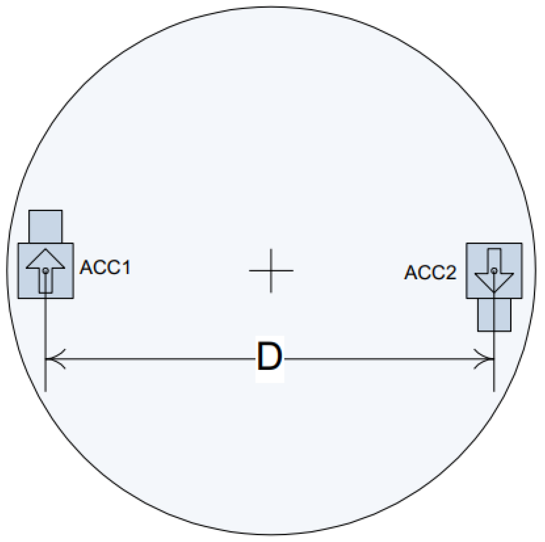
| Two linear accelerometers | Circular motion | Easy to operate; Large installation error. | ★ |
| Free-oscillation method | Torsion pendulum principle | Inconsecutive frequency; Complex operation | ★ |
| Self-calibratable rotary encoder | Equal division averaged method | Self-calibration; Easy to operate; Only suitable for medium-performance MEMS gyroscopes. | ★ |
| Frequency (Hz) | THD (%) | |||||
|---|---|---|---|---|---|---|
| No Additional Load | One Disk | Two Disk | ||||
| Motor | Angular | Motor | Angular | Motor | Angular | |
| Current | Acceleration | Current | Acceleration | Current | Acceleration | |
| 21 | 0.011% | 0.040% | 0.009% | 0.021% | 0.010% | 0.017% |
| 41 | 0.007% | 0.011% | 0.007% | 0.010% | 0.008% | 0.011% |
| 61 | 0.008% | 0.008% | 0.007% | 0.010% | 0.008% | 0.011% |
| 81 | 0.007% | 0.010% | 0.007% | 0.012% | 0.007% | 0.012% |
| 101 | 0.007% | 0.011% | 0.007% | 0.013% | 0.007% | 0.013% |
| 211 | 0.007% | 0.024% | 0.006% | 0.027% | 0.007% | 0.026% |
| 411 | 0.008% | 0.063% | 0.007% | 0.061% | 0.008% | 0.059% |
| 611 | 0.014% | 0.102% | 0.014% | 0.097% | 0.015% | 0.093% |
| 811 | 0.024% | 0.138% | 0.024% | 0.136% | 0.024% | 0.118% |
| 1011 | 0.035% | 0.172% | 0.035% | 0.164% | 0.034% | 0.135% |
| 1211 | 0.041% | 0.200% | 0.041% | 0.180% | 0.042% | 0.148% |
| 1411 | 0.047% | 0.236% | 0.046% | 0.213% | 0.046% | 0.268% |
| 1611 | 0.048% | 0.258% | 0.048% | 0.204% | 0.048% | 0.219% |
| 1811 | 0.049% | 0.287% | 0.048% | 0.607% | 0.048% | 0.513% |
| 2011 | 0.047% | 0.340% | 0.047% | 0.282% | 0.045% | 2.383% |
| Number | Frequency = 36 Hz | Frequency = 101 Hz | Frequency = 601 Hz | |||
|---|---|---|---|---|---|---|
| Amplitude | Phase | Amplitude | Phase | Amplitude | Phase | |
| (mrad/s) | () | (mrad/s) | () | (mrad/s) | () | |
| 1 | 26.397 | 144.453 | 8.835 | 102.891 | 1.458 | 57.466 |
| 2 | 26.400 | 144.396 | 8.835 | 102.313 | 1.352 | 59.502 |
| 3 | 26.401 | 144.605 | 8.835 | 102.373 | 1.458 | 59.426 |
| 4 | 26.402 | 144.684 | 8.834 | 102.940 | 1.461 | 59.640 |
| 5 | 26.401 | 144.493 | 8.835 | 103.274 | 1.457 | 57.590 |
| Mean | 26.400 | 144.526 | 8.835 | 102.758 | 1.437 | 58.725 |
| Standard Deviation | 1.924 | 0.117 | 4.471 | 0.407 | 4.765 | 1.096 |
| Frequency = 46 Hz | Frequency = 201 Hz | Frequency = 401 Hz | ||||
|---|---|---|---|---|---|---|
| Amplitude | Phase | Amplitude | Phase | Amplitude | Phase | |
| (V/(rad/s)) | () | (V/(rad/s)) | () | (V/(rad/s)) | () | |
| Mean | 0.610 | 1.551 | 0.604 | 164.650 | 0.548 | 147.691 |
| Standard Deviation | 6.23 | 0.119 | 3.00 | 0.396 | 7.20 | 0.720 |
| Source of Uncertainty | Distribution | Type of Evaluation Method | Relative Standard Uncertainty Value | |
|---|---|---|---|---|
| A/D digits of the data acquisition card | Uniform | B | ||
| Voltage noise of sensor | Uniform | B | ||
| Repeatability error of voltage amplitude measurement | Normal | A | ||
| Vibration interference | Normal | B | ||
| Principle error of chord length replacing arc length | Uniform | B | ||
| Mounting error of optical device | Uniform | B | ||
| Noise of photoelectric signal | Uniform | B | ||
| Vibration interference | Normal | B | ||
| Manufacturing deviation of angular retroreflector | Uniform | B | ||
| Change in air refractive index | Uniform | B | ||
| Repeatability error of angle measurement | Normal | A | ||
| Accuracy of frequency | Normal | B |
© 2019 by the authors. Licensee MDPI, Basel, Switzerland. This article is an open access article distributed under the terms and conditions of the Creative Commons Attribution (CC BY) license (http://creativecommons.org/licenses/by/4.0/).
Share and Cite
Wu, Y.; Li, X.; Liu, F.; Xia, G. An On-Orbit Dynamic Calibration Method for an MHD Micro-Angular Vibration Sensor Using a Laser Interferometer. Sensors 2019, 19, 4291. https://doi.org/10.3390/s19194291
Wu Y, Li X, Liu F, Xia G. An On-Orbit Dynamic Calibration Method for an MHD Micro-Angular Vibration Sensor Using a Laser Interferometer. Sensors. 2019; 19(19):4291. https://doi.org/10.3390/s19194291
Chicago/Turabian StyleWu, Yingjie, Xingfei Li, Fan Liu, and Ganmin Xia. 2019. "An On-Orbit Dynamic Calibration Method for an MHD Micro-Angular Vibration Sensor Using a Laser Interferometer" Sensors 19, no. 19: 4291. https://doi.org/10.3390/s19194291
APA StyleWu, Y., Li, X., Liu, F., & Xia, G. (2019). An On-Orbit Dynamic Calibration Method for an MHD Micro-Angular Vibration Sensor Using a Laser Interferometer. Sensors, 19(19), 4291. https://doi.org/10.3390/s19194291