Article

Gunshot Airborne Surveillance with Rotary Wing UAV-Embedded Microphone Array

by
Felipe Gonçalves Serrenho
1,*,
José Antonio Apolinário, Jr.
1,
António Luiz Lopes Ramos
2 and
Rigel Procópio Fernandes
3
1
Department of Electrical Engineering, Military Institute of Engineering (IME), Rio de Janeiro 22290-270, Brazil
2
Department of Science and Industry Systems, University of South-Eastern Norway (USN), 3616 Kongsberg, Norway
3
Program of Defense Engineering, Military Institute of Engineering (IME), Rio de Janeiro 22290-270, Brazil
*
Author to whom correspondence should be addressed.
Sensors 2019, 19(19), 4271; https://doi.org/10.3390/s19194271
Submission received: 23 August 2019 / Revised: 19 September 2019 / Accepted: 24 September 2019 / Published: 1 October 2019

Abstract

:
Unmanned aerial vehicles (UAV) are growing in popularity, and recent technological advances are fostering the development of new applications for these devices. This paper discusses the use of aerial drones as a platform for deploying a gunshot surveillance system based on an array of microphones. Notwithstanding the difficulties associated with the inherent additive noise from the rotating propellers, this application brings an important advantage: the possibility of estimating the shooter position solely based on the muzzle blast sound, with the support of a digital map of the terrain. This work focuses on direction-of-arrival (DoA) estimation methods applied to audio signals obtained from a microphone array aboard a flying drone. We investigate preprocessing and different DoA estimation techniques in order to obtain the setup that performs better for the application at hand. We use a combination of simulated and actual gunshot signals recorded using a microphone array mounted on a UAV. One of the key insights resulting from the field recordings is the importance of drone positioning, whereby all gunshots recorded in a region outside a cone open from the gun muzzle presented a hit rate close to 96%. Based on experimental results, we claim that reliable bearing estimates can be achieved using a microphone array mounted on a drone.

1. Introduction

The interest in automatic sniper localization systems traces back to the early 1990s, pioneered by countries such as the United States of America, Russia, Canada, France, and more recently, Israel, among others. Such surveillance systems for shooter detection and localization can be useful to the police and military forces [1,2]. The shooter detection and localization problem can be approached in different ways, depending on the kind of signatures from a gunshot event, acoustic or electromagnetic, that one decides to process [3]. For instance, cameras can be used to detect the muzzle flash [4], whereas microphone arrays can be used to detect the muzzle blast and the shockwave acoustic signatures. If these two acoustic signatures are detected in the same gunshot event, one can estimate the location of the shooter using a two-step procedure [3].
The successful use of microphone arrays to tackle the direction-of-arrival (DoA) estimation problem even with low signal-to-noise ratio (SNR) can be seen in Reference [5]. In this paper, median filtering is used to enhance the collected acoustic gunshot signals. In Reference [6], an algorithm that optimizes DoA estimation using exhausive search through consistent fundamental loops is introduced. This method, in an attempt to have the best approach for the level of noise of audio signals, is a combination of standard DoA estimation, Exhaustive Search (ES) [7], and consistent fundamental loop [6].
Microphone arrays can be deployed in different platforms, e.g., stand-alone systems mounted on vehicles [8], on light posts in urban areas or on trees in a forest [9]. All these systems are currently subjects of great interest in academia and are recently associated with the internet of things (IoT) industry [10] as well. However, one such system based on a microphone array mounted on an aerial drone brings additional advantages owing to its flexibility to cover wider areas relatively quicker and at a lower cost. It also opens the opportunity for new important applications, such as search-and-rescue missions [11,12] and environmental monitoring [9]. In Reference [11], a microphone array mounted on a drone is used to detect a narrowband signal generated by a whistle, which can be very effective in search-and-rescue missions in areas of difficult access.
An application example for environmental monitoring is presented in Reference [9], suggesting the use of an open hardware to be deployed in the forest to record audio signals and using a Secure Digital (SD) card to store the data. These signals vary from bat ultrasounds to gunshot signals. For instance, in the case of detecting gunshot events in protected areas, people responsible for monitoring those areas could be triggered to carry out necessary actions against poaching. Hoshiba et al. presented detailed design and implementation of a quadcopter-embedded microphone array system for outdoor environments [12].
In order to enable new drone applications, the scientific community has developed an interest for new techniques capable of tackling the strong ego-noise presented in audio recordings from unmanned aerial vehicle (UAV)-embedded microphone arrays, especially when the target sound is a whistle or human speech. Methods based on Multiple Signal Classification (MUSIC), known to be very robust against noise, are presented in Reference [13]. The Generalized Eigenvalue Decomposition-MUSIC (GEVD-MUSIC) [14,15] is reported to have high performance even for low-SNR signals. The incremental Generalized Eigenvalue Decomposition-MUSIC (iGEVD-MUSIC) introduced in Reference [16] estimates the noise correlation matrix incrementally to cope with the high non-stationarity of the ego-noise. A supervised approach that uses UAV sensors data and motor rotation speeds to estimate the noise correlation matrix was proposed in Reference [17]. Aiming at reducing computational complexity and errors associated with inaccuracies in noise correlation matrix estimation, Reference [18] proposes the Multiple Signal Classification based on incremental Generalized Singular Value Decomposition-MUSIC (iGSVD-MUSIC) with Correlation Matrix Scaling (CMS).
A novel algorithm to sound source location with UAV-embedded microphone arrays based on time-frequency bins was proposed in Reference [19]. This method takes advantage of the fact that ego-noise and target sound (e.g., speech or emergency whistle) mainly consist of harmonic components that usually occupy different time-frequency bins. In Reference [20], the time-frequency technique is associated with a time-frequency spatial filter to enhance the signal of interest. Other interesting researches related to sound processing with drones include the following: a study about the ego-noise of multirotors micro aerial vehicles [21], that also proposes the use of Blind Source Separation (BSS) algorithm to suppress it; the use of ego-noise to measure the relative directions between multirotors in a swarm [22]; and the ability to track moving sound sources [23].
Focusing on gunshot airborne surveillance, the deployment of acoustic sensors in elevated platforms could enable advantages for shooter-position estimation, according to Reference [24]. The use of an aerial drone as a mobile elevated platform was investigated in Reference [25], using only simulations. Different noise levels were synthesized using drone noise recordings in a silent room and real gunshot signals recorded with a high-quality microphone mounted on a tripod in an open field. Also in this work, signal enhancement techniques were employed along with DoA estimation algorithms and target motion analysis was used to estimate the shooter’s position. In Reference [26], the geometry deployment of the microphone array is discussed, taking into account the wind produced by the propellers, the electromagnetic interference, and the scarce space available on the drone.
In this paper, we focus on the details of DoA estimation of gunshot signals obtained from a microphone array aboard a flying drone. We used simulations to investigate the performance of preprocessing and DoA estimation techniques, also tuning theirs parameters. The most appropriated methods were evaluated with actual field recordings, given the position and attitude of the drone obtained from its GPS and inertial unit.
The rest of this paper is organized as follows. Section 2 starts with a brief overview on gunshot acoustics, followed by a discussion on the techniques used in a UAV-based gunshot surveillance system, namely signal preprocessing, gunshot detection, DoA estimation, and shooter localization. Section 3 describes the hardware used and the shooting site as well as how telemetry data is recovered and used, while Section 4 discusses experimental results from simulations and from actual gunshot signals collected using an array of sensors mounted on a flying drone. The discussion and conclusion are addressed in Section 5.

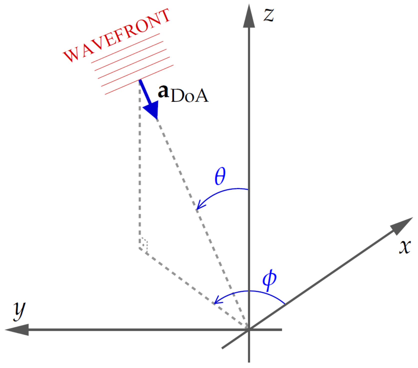
2. DoA Estimation and Shooter Localization
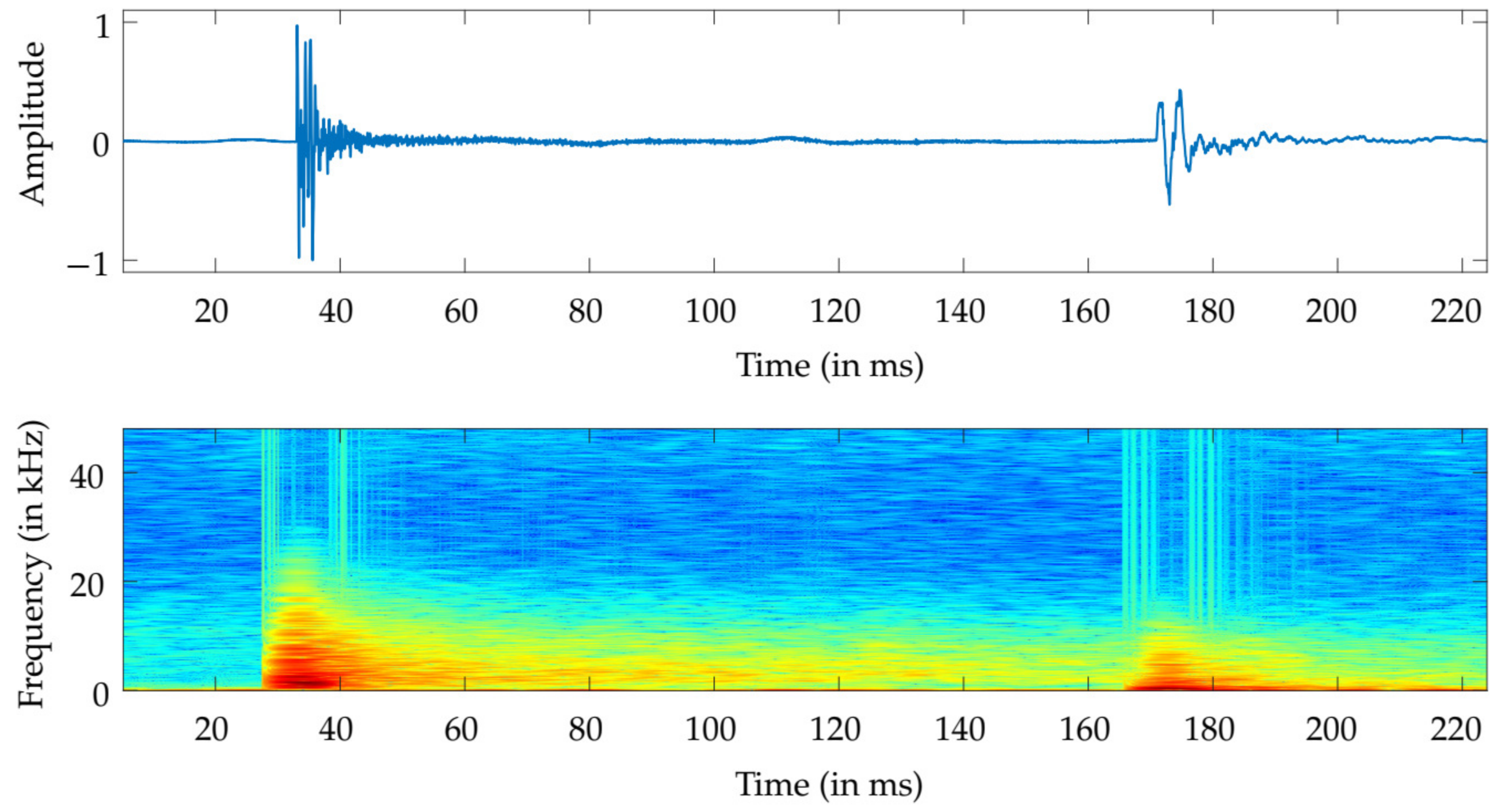
The acoustic signatures generated by a gunshot event can be divided into three parts, namely the muzzle blast, the shockwave, and sounds related to mechanical actions, which include the trigger and hammer mechanisms, ejection of spent cartridges, and the loading system. The mechanical action-related sounds can be useful in forensics analysis [27,28]. However, they are of no interest in the design of sniper localization systems, since they can only be recorded using sensors placed close to the gun.
The muzzle blast is generated by the expansion of gases in the gun barrel and is louder in the direction the barrel is pointing toward [29,30]. It propagates at the speed of sound and lasts typically from 3 to 5 ms [31]. The energy of the muzzle blast depends on the firearm used, and it is almost always audible in a given range, provided that silencers or suppressors are not used [31,32].
A shockwave will be generated for as long as a projectile is travelling faster than the speed of sound and propagates outwards from the bullet trajectory at an angle known as the Mach angle [33]. The shockwave generated by a typical supersonic bullet lasts for approximately 200 µs, and its frequency spectrum has a wider frequency band than that of the muzzle blast, as exemplified in Figure 1. Since the shockwave propagates in a cone shape following the bullet trajectory, it cannot be detected if the bullet is moving away from the position where the sensors are located [34]. This constitutes a problem for shooter localization systems that rely on the detection of both shockwave and muzzle blast signals.
The shooter’s localization problem may be divided in four steps, namely preprocessing, gunshot detection and muzzle blast identification, DoA estimation, and shooter-position estimation.

2.1. Preprocessing

Localization of a shooter based on the audio acquired from a drone is especially challenging due to the presence of strong ego-noise, mainly generated by the propellers [35]. This becomes an even greater challenge under long-range shootings, whereby the detection and the direction-of-arrival estimation of the muzzle blast signal is compromised.
When signals of interest are approximately stationary, such as tiny voice snippets, whistles, or white noise, methods based on noise correlation matrix estimation, such as Wiener Filtering [36], are used. For impulsive signals, as in the case of gunshot signals, median filtering is an alternative option [5]. In this work, we evaluate the performance of these methods in the task of DoA estimation.
During steady parts of a flight, where stationarity can be assumed [36], we may use Wiener filtering to attenuate the influence of the ego-noise. We used in this work the implementation developed by Liu Ming and Pascal Scalart [37,38]. This Wiener filter, referred to as Two-Step Noise Reduction (TSNR), uses the decision-directed approach [39] to track a priori SNR and refines the SNR estimation to avoid reverberation effects.
Median filtering was employed in Reference [40] as a technique to separate percussive and harmonic components of a signal. The proposed scheme uses the concept that percussive components can be seen as outliers in the time domain while harmonic sounds can be seen as outliers in the frequency domain. Median filtering, described next, is capable of removing these outliers and of separating these different acoustic signatures to some extent. Given the input x ( k ) , the output y ( k ) is the median value of the window with length Δ centered in x ( k ) . The parameter should be chosen accordingly, in such a way that the expected duration of the artifacts is removed but without significant impact on the signal of interest. The median filtering can be expressed according to the following:
y ( k ) = m e d i a n { x ( k l : k + l ) } , l = ( Δ 1 ) / 2 , if Δ is   odd ;
if Δ is even, the median is defined as the mean of the two central median values.
The use of median filtering to estimate background noise embedded in gunshot signals was introduced in Reference [5], which computes the enhanced signal as s ( k ) = x ( k ) y ( k ) . To preserve the muzzle blast’s shape, Δ should not represent less than half of its duration, which is approximately 3 ms [31].

2.2. Gunshot Detection

As previously noted, a gunshot surveillance system must be able to detect an impulsive signal and to identify if it is a muzzle blast component, a shockwave component, or none of them. There is a vast literature available about this matter [41,42,43,44,45,46].
The method in Reference [41] uses a transient detection, introduced in Reference [42], that looks for significant changes in the signal energy. For muzzle blast and shockwave classification, Reference [41] uses two tests: the first one is based on the spectral information of the signal, and the second one uses time difference of arrival between neighboring peaks.
A detection scheme based on correlation against a template is proposed in Reference [43], where the authors claim that the method could be implemented by a low power consuming hardware. Correlation against a template is also addressed in Reference [44], where it is compared against classical algorithms usually used in speech processing; their results conclude that correlation matches the performance of those algorithms, especially in noisy environments. In Reference [45], linear predictive coding (LPC) coefficients are combined with template matching to increase the performance of gunshot detection systems, especially regarding false-positive errors.
A wavelet-based approach [46] can be used to distinguish three acoustic events: muzzle blast, shockwave, and reflections. Furthermore, according to the authors, this method can classify the caliber based on the muzzle blast or on the shockwave signals.
The strong ego-noise of a drone is not white and is highly nonstationary [36]. Furthermore, it is strongly dependent on the drone used and on the positioning of the sensors. These are additional challenges to detection and muzzle blast–shockwave classification. These tasks were carried out manually in this work.

2.3. DoA Estimation Methods

In this section, we first define DoA angles and then present two DoA estimation methods: a data selection least squares method [7] and an angular spectrum-based method named the Multi-channel Blind Source Separation (MBSS) Locate [47].
Figure 2 shows the angles (azimuth ϕ and zenith θ ) that define the DoA. It is noteworthy that the azimuth herein is taken counterclockwise, as in Reference [48]. Thus, the unit vector in the direction of sound wave propagation is given as follows:
a DoA = cos ( ϕ ) sin ( θ ) sin ( ϕ ) sin ( θ ) cos ( θ ) T .

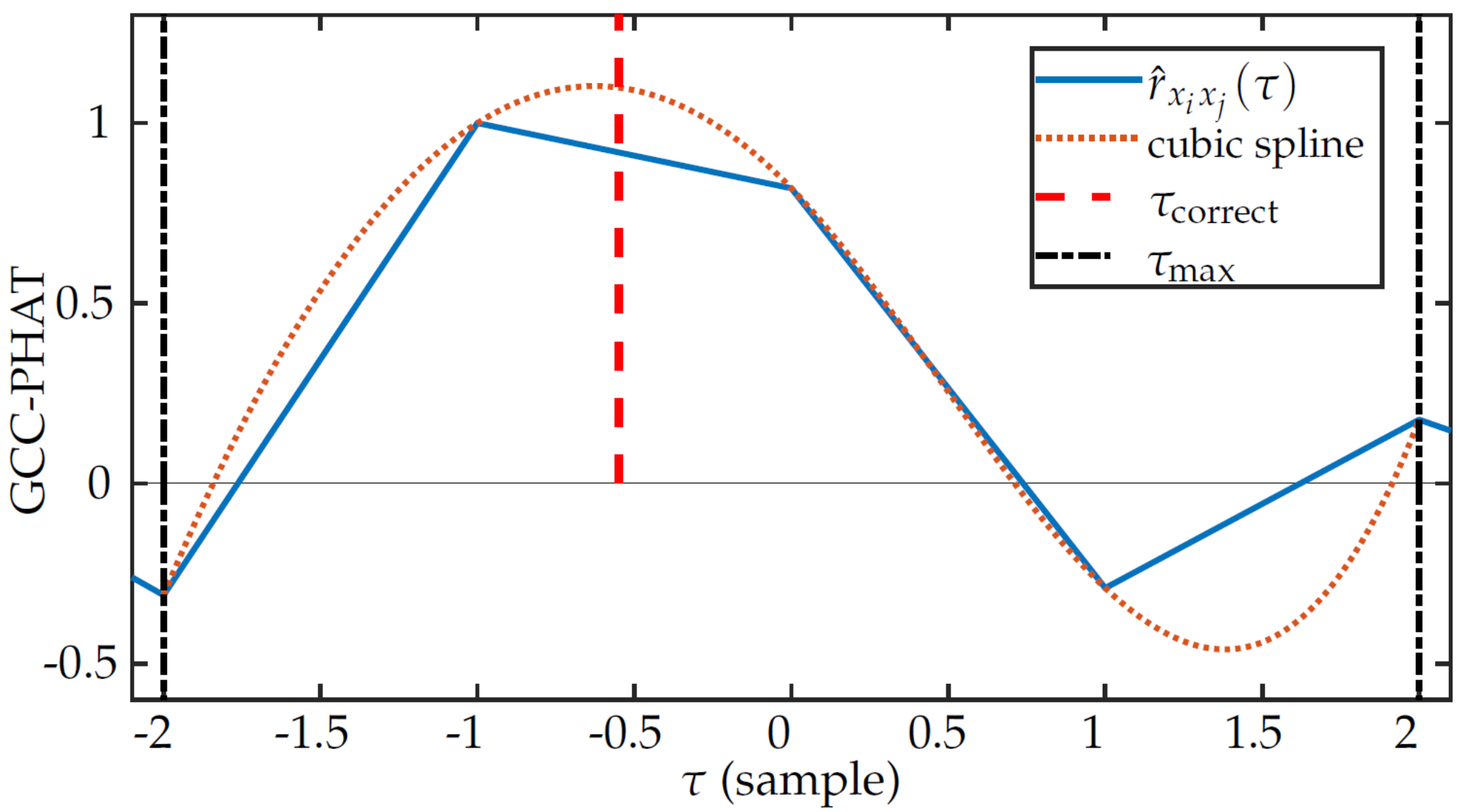
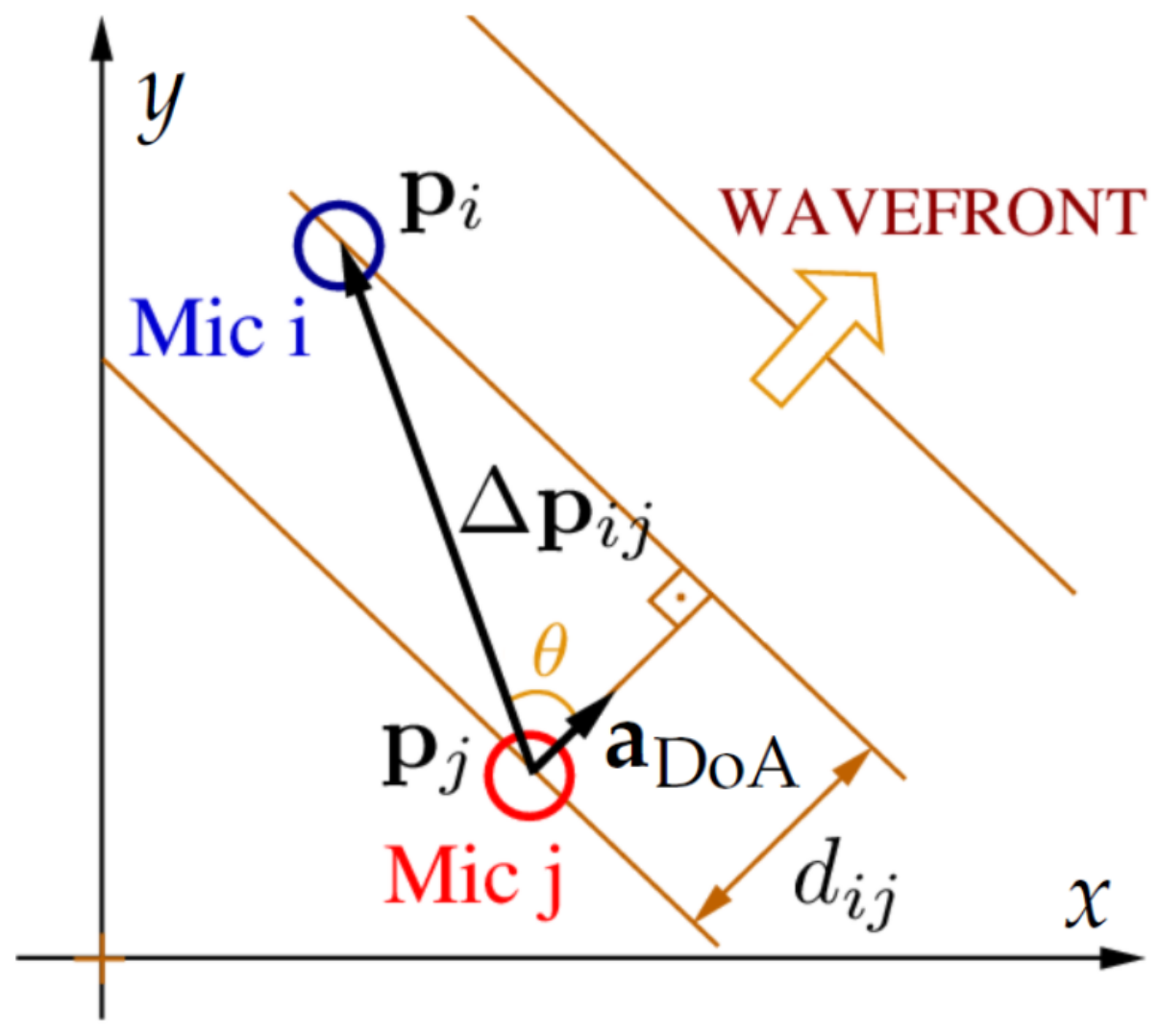
2.3.1. The Data Selection Least Squares DoA Estimation Algorithm

The first step of the least squares (LS) method is the time-delay estimation (TDE) between the sensor pairs in the array. Next, we use an LS cost function associated with a data-selective algorithm. The TDEs are obtained from the peak of the cross-correlation r x i x j ( τ ) defined as follows [49]:
r x i x j ( τ ) = E [ x i ( k ) x j ( k τ ) ] ,
where E denotes the expectation operator and τ is the lag between two given sensors, x i and x j . In practice, we do not have statistical knowledge of the signals, and Equation (3) is usually approximated by its time average given by the following:
r ^ x i x j ( τ ) = k = x i ( k ) x j ( k τ ) = x i ( τ ) * x j ( τ ) ,
where * is the convolution operator.
Taking the discrete Fourier transform of r ^ x i x j ( τ ) and assuming real-valued signals, we can write the cross power spectrum density between x i ( k ) and x j ( k ) as follows:
R ^ x i x j ( e j w ) = F { r ^ x i x j ( τ ) } = F { x i ( τ ) * x j ( τ ) } = X i ( e j w ) X j ( e j w ) = X i ( e j w ) X j * ( e j w ) .
The cross-correlation can then be computed using the following:
r ^ x i x j ( τ ) = F 1 { R ^ x i x j ( e j w ) } .
Adding a frequency weighting function in Equation (6), we have the generalized cross-correlation (GCC) as follows:
r ^ x i x j ( τ ) = F 1 { ψ ( w ) R ^ x i x j ( e j w ) } ,
where classical cross-correlation corresponds to ψ ( w ) = 1 , w . A popular weighting scheme employed by the GCC is the phase transform (PHAT) [7,36,49,50,51,52,53], known to have good performance in reverberating scenarios [49]. PHAT also tends to have a sharper peak than classical GCC, increasing the performance of the TDE [50]. The PHAT weighting function is given by the following [53]:
ψ PHAT ( w ) = 1 | X i ( e j w ) X j ( e j w ) | .
Finally, the TDE is obtained as follows:
τ ^ i j = arg max | τ | τ max | r ^ x i x j PHAT ( τ ) | ,
where τ max is the maximum delay possible (in number of samples) between microphone i and j, which occurs when the DoA has the same direction of the vector that connects sensors i and j:
τ max = | p i p j | f s v s ,
where p i and p j are the position vectors of sensors i and j, v s is the speed of sound, and f s is the sampling frequency. The TDEs using inverse Fourier transform (iFFT) provide delays as integer multiples of the sampling period; this leads to errors that are particularly relevant in small arrays (small time delays between sensors) and with low sampling frequency. To mitigate this source of errors, we can interpolate the GCC, allowing more accurate estimations of the time difference of arrival (TDoA). In this work, we used cubic interpolation [54], calculated at every point in between τ max and τ max , ensuring that all possible values of delay are covered. Figure 3 shows the effect of cubic interpolation over GCC-PHAT in a small array for a signal with f s = 8 kHz.
Figure 4 illustrates in 2-D the delay between microphones i and j. In a 3-D scenario, we write d i j = Δ p i , j T a DoA such that the TDE (in samples) is given by the following:
τ i , j = f s ( p i p j ) T a DoA v s = f s Δ p i , j T a DoA v s = Δ p ¯ i , j T a DoA ,
where Δ p ¯ i , j = f s Δ p i , j / v s .
Based on the estimated delay, as given in Equation (9), and the delay based on the unknown vector a DoA , Equation (11), we define the least squares cost function:
ξ = i , j ( τ i , j Δ p ¯ i , j T a DoA ) 2 ,
for all possible pairs, N = M ( M 1 ) / 2 for the case of M microphones.
Minimizing the cost function with respect to a DoA , we find the following:
a DoA = R 1 d ,
where d = Δ p ¯ T τ , τ = [ τ 1 , 2 τ 1 , 3 τ 1 , N τ 2 , 3 τ M 1 , M ] T and R = Δ p ¯ T Δ p ¯ , Δ p ¯ are assembled as follows:
Δ p ¯ = Δ p ¯ 1 , 2 Δ p ¯ 1 , 3 Δ p ¯ 1 , M Δ p ¯ 2 , 3 Δ p ¯ M 1 , M T .
The solution provided by Equation (13) may not have unit norm, which must be ensured through normalization. Only then could azimuth and zenith be calculated using trigonometric operations, according to Equation (2).
Equation (13) provides all three coordinates only when using a spatial array. If a planar array is used, ambiguity occurs and matrix R is singular. When all sensors are in a plane ( x y -plane for instance), we must adapt the sensor positions ( p i ) to suppress the coordinate associated with the perpendicular axis, in our case z. This way R is non-singular and Equation (13) provides a ^ DoA incomplete = [ a x a y ] T . As the a DoA must be unitary and assuming that the source is located above or below the array, it is possible to estimate the DoA.
The strong ego-noise could compromise the TDEs, generating outliers that would adversely affect the DoA estimation. As for the cost function defined in Equation (12), the solution can be obtained without using all available pairs of microphones; it is possible to use a data-selective algorithm to remove outliers. Using the Exhaustive Search algorithm ES(n) [7], we choose the n combination from the set of N pairs of microphones that minimizes the cost function ξ in Equation (12). We need to be cautious when choosing the number of pairs of microphones to be used, parameter “n” in ES(n), once it can generate ill-conditioned matrices [55]. The appropriate choice for “n” can be obtained according to a decision tree as done in Reference [6].

2.3.2. The MBSS Locate

The Multi-channel Blind Source Separation (MBSS) Locate [56] is available as a MATLAB ® toolbox. It estimates the direction of arrival of multiple sources from audio signals collected by an acoustic sensor array. This software implements multichannel versions of four state-of-the-art and three proposed SNR-based local angular spectra methods for audio signals [47].
The state-of-the-art local angular spectra methods are GCC-PHAT [49] and its version with a nonlinear function GCC-NONLIN [57], Multiple Signal Classification (MUSIC) [13], and Cumulative State Coherence Transform (cSCT) [58]. These techniques, except the cSCT method, rely on the assumption that one source is predominant in each time-frequency bin. The cSCT method assumes that there are at most two predominant sources.
The SNR-based local angular spectra tackles the multisource TDoA estimation problem. The main idea is to use the SNR as an unbounded measure to estimate if the information of a time-frequency bin results from a single source. Blandin et al. [47] proposed three methods to estimate the SNR using two microphones and the following techniques: Minimum Variance Distortionless Response (MVDR) [59], Diffuse Noise Model (DNM) [60], and Minimum Variance Distortionless Response Weighted (MVDRW).
The MBSS full version enables the user to simulate the recording scenario, e.g., room dimensions, walls absorption coefficient, and number of microphones [56]. Nevertheless, we summarize in the following only the core of the angular-spectra based method. For detailed information about its functionalities and implementation, one should refer to the user guide provided with the software.
We describe the use of the MBSS algorithm in three main steps. The first step is to define the possible angles of azimuth and zenith and to assemble the search grid. The program uses elevation instead of zenith, but it can be easily converted: zenith = π 2 − elevation. Based on the grid, the set of possible delays for each pair of microphones is computed, and then, it is resampled to limit the quantity to points in which angular spectrum is calculated. The software offers some options to compute angular spectra. For this work, we used the GCC-PHAT local angular spectra defined as follows [47]:
γ i , j PHAT ( l , f , t ) = R R ^ x i x j ( l , f ) | R ^ x i x j ( l , f ) | e 2 π f t
where R is the real operator, l is the index of the time frame, f is the center frequency of the FFT bin, and t is the delay in seconds.
In the second step, the contents of all selected frequency bins are summed up. A linear interpolation is used in γ i , j PHAT ( t , l ) to the compute angular spectrum approximation in all possible t in each pair of microphones. This value is used to calculate the angular spectrum directly, depending on the direction of arrival, γ i , j ( l , ϕ , θ ) . Then, angular spectrum of all pairs are summed, generating γ ( l , ϕ , θ ) . For multiple time frames, there are two strategies: sum all time frames or use the maximum overall time frames. The last one is recommended when the signal of interest is only active in a few frames [47]. As the gunshot signals are impulsive, the maximum approach was used and the angular spectrum is then given by the following:
γ max ( ϕ , θ ) = max l γ PHAT ( l , ϕ , θ ) .
The last step of the MBSS algorithm is a grid search to find the global maximum in the case of only one source or the local maxima when there are multiple sources. If there is only one single source, the DoA angles are obtained from the following:
ϕ ^ , θ ^ = arg max ϕ , θ γ ( ϕ , θ ) .

2.4. Position Estimation

There are a number of ways to estimate the shooter localization. A simple approach uses DoA estimations of muzzle blast from different arrays according, for instance, to the total least squares (TLS) [61] algorithm. Since this method does not use the shockwave component, it can estimate position even of small caliber weapons of which the projectiles do not reach supersonic speed. Another advantage of this method is that, with a sufficient number of arrays, it could be combined with a data-selective algorithm, such as Exhaustive Search, seen in Section 2.3, to remove outliers expected to happen when some arrays do not have a clean sight to the firearm or are heavily affected by multipath [31,32]. On the other hand, in order to use the TLS approach, the system would be more complex and expensive to be deployed, since it requires more than one drone and they need to communicate with the node responsible for the calculation of the shooter’s position with the information of all platforms.
A second approach is to combine shockwave and muzzle blast DoA estimations to compute the probable shooter location [41,62]. As this method uses shockwave components, it is only applicable in the case of supersonic projectiles and when the array is inside the shockwave field of view. Moreover, this method assumes (at least its simplest version) that the projectile has a constant speed, which tends to generate results that overestimate the distance when the shooter is more than 100 m from the array; adaptations are then required to overcome this limitation as stated in Reference [63].
A third approach presented in Reference [24] combines muzzle blast DoA estimation from an elevated array with a digital map containing topographic information to estimate the shooter position. The main concern of this method is to obtain the appropriate digital model of the terrain. As in the TLS approach, this method can estimate the position of subsonic firearms. This approach would be appropriated for our scenario, but focusing on the DoA estimation, we have not carried out a position estimation evaluation in this work.

3. System Setup and Signal Acquisition

In this section, we describe the hardware, the drone, and the microphone array used in field recordings. We also provide some information about the shooting site and the environmental conditions the experiment was performed under. We also provide details regarding the data acquisition process, including audio recording and drone flight log data.

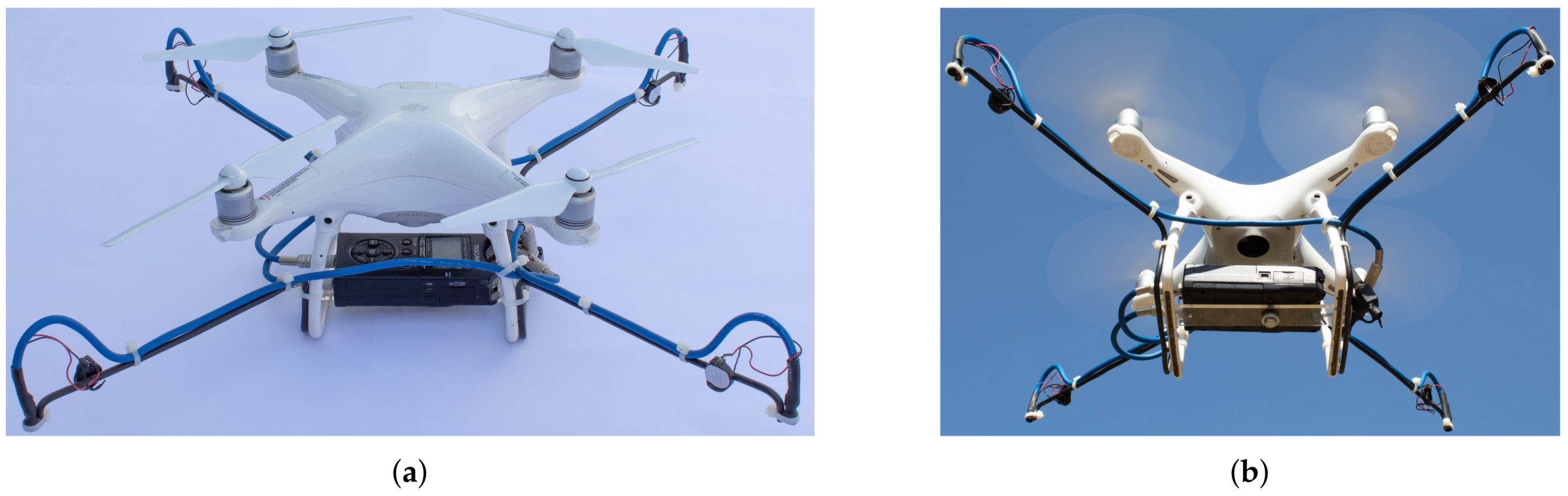
3.1. UAV and Avionics

We used a DJI Phantom 4. It weights 1.38 kg (battery and propellers included but without the extra hardware used for recording the audio signals) and has a 35 cm diagonal, also featuring a 4K camera, and support for two satellite positioning systems (GPS nad GLONASS). According to the manufacturer [64], the UAV, without any external hardware, is able to resist to wind gusts up to 36 km/h.
The microphone array was mounted in 41 cm metal rods, aligned with the propeller’s arms. The size of the rods was engineered to keep the microphones away from the propellers to reduce the influence of noise caused by air displacement generated by the rotating blades. The four microphones were placed in the same height in a planar structure to avoid interference with the drone’s maneuverability, especially during take off and landing. The planar coordinates for the microphones are given in Table 1, assuming the origin of the coordinate system in the center of the UAV.
The gimbal and the camera were removed, allowing the recorder to be placed under the drone (see Figure 5), aligning it with the center of mass of the multirotor, and minimizing the impact on the flight capabilities of the UAV. Care was taken in order not to cover the ultrasonic sensors, located on the underside of the drone’s hull; this would severely affect flight safety and its landing ability.

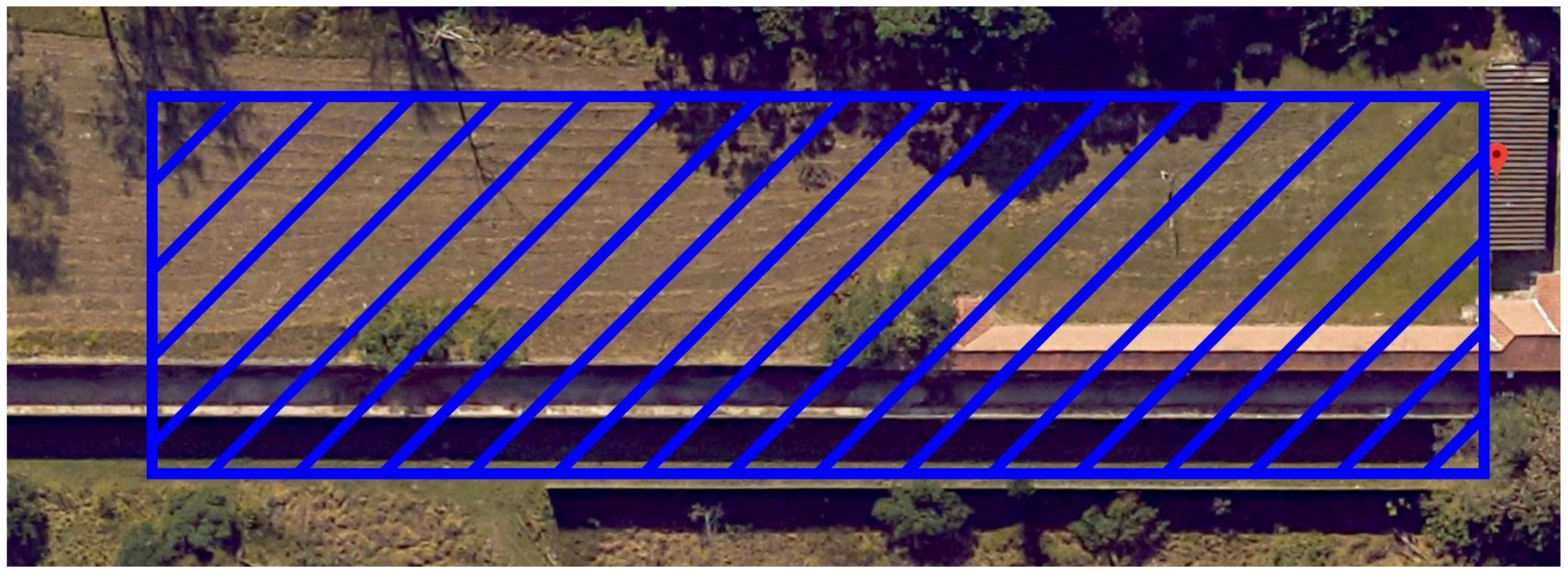
3.2. Environmental Conditions and Shooting Site

The gunshot signals were collected in a shooting site located at the Brazilian Army Evaluation Center (CAEx) on a cloudy day with no strong wind and with a temperature of 24 ° C. Figure 6 shows a satellite image of the shooting site. The drone’s flight zone was restricted to the blue rectangle of area 30 × 120 square meters to prevent it from flying over sensitive regions and to ensure a clear line of sight to the shooter.

3.3. Data Acquisition: Audio and Drone Position and Attitude
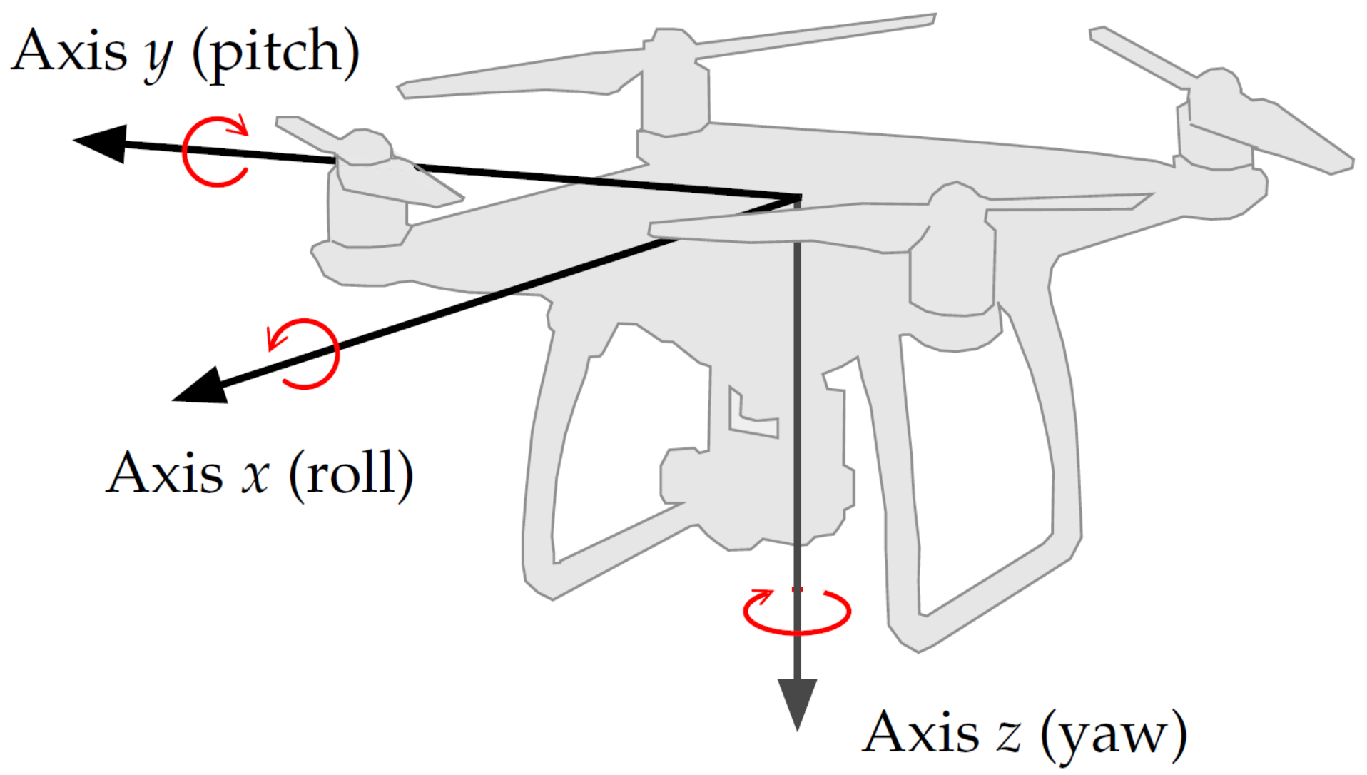
The four microphones were connected to a four-channel recorder, TASCAM DR-40 [66], which is convenient given its relatively reduced dimensions and light weight of 0.213 kg without batteries. The TASCAM DR-40 recorder comes with two connectors for external microphones and two built-in microphones, which were rearranged to a single set with four external channels to accommodate four small electret microphones.
The recordings were carried out using a sampling frequency of 44.1 kHz and encoded using 24 bits per sample. The drone flight log data was recorded in a file and recovered using AirData.com [67]. The log data provides the following information: time (in ms), GPS coordinates (latitude and longitude), altitude, and attitude data (angles yaw, roll, and pitch), as illustrated in Figure 7.
The digital audio recorder and the drone were initialized manually and simultaneously for each flight to synchronize the data about the position and the attitude of the drone with the recorded gunshot signals. As the drone was hovering when the shots were fired, the mismatch due to the manual process is negligible. Furthermore, there was no considerable drift caused by two different clocks, since the battery capacity limits the duration of each flight to a maximum of 18 minutes.

3.4. Axis Rotation

The DoA is calculated with respect to the drone’s coordinates of which the axes are not necessarily aligned with the geographic axes. Therefore, after calculating the DoA with respect to the drone’s coordinates, we must rotate the DoA vector in order to match the orientation of the geographic axes. The rotation can be applied by a series of matrix multiplications [69], using the attitude data and the magnetic declination of the location. Considering the axes system shown in Figure 2, the matrix that computes a rotation over axis z (yaw- α ) is given by the following:
R z ( α ) = cos ( α ) sin ( α ) 0 sin ( α ) cos ( α ) 0 0 0 1 ,
The rotation matrix over axis y (pitch- β ) is given by the following:
R y ( β ) = cos ( β ) 0 sin ( β ) 0 1 0 sin ( β ) 0 cos ( β ) ,
Also, the matrix that performs the rotation over axis x (roll- ψ ) is given by the following:
R x ( ψ ) = 1 0 0 0 cos ( ψ ) sin ( ψ ) 0 sin ( ψ ) cos ( ψ ) .
Therefore, the rotated DoA vector in the geographic coordinate system is expressed as follows:
a DoA rotated = R z ( α ) R y ( β ) R x ( ψ ) a DoA drone .
Please note that matrix multiplication is not commutative, and therefore, the sequence roll, pitch, and yaw must be respected. Furthermore, the coordinates systems in Figure 2 and Figure 7 are not the same: axes y and z point in opposite directions; it is necessary to reverse the rotation directions of pitch and yaw angles given by DJI Phantom 4. We must also take into account magnetic declination when rotating over axis z Equation (18), or the DoA vector will be aligned with magnetic north instead of geographic north.

4. Experimental Results

4.1. Simulated Signals

In this work, we used simulated muzzle blast gunshot signals with different noise levels to tune parameters and to evaluate the performance of DoA estimation methods. In order to evaluate the quality of a DoA estimation, we used the angle between the estimated and the actual DoA, herein named angular error and defined as follows:
Angular   Error = cos 1 a DoA T a ^ DoA ,
where a DoA is the correct DoA vector and a ^ DoA is the estimated one. Angular error can vary from 0 ° , when there is no error in DoA estimation, up to 180 ° , when DoA estimation points towards the opposite direction of actual DoA. This metric allows us to compare objectively two different estimations while avoiding distortions in azimuth error when zenith is close to 0 ° or 180 ° . We used three performance measures based on angular error to evaluate the DoA estimation methods: mean, standard deviation, and percentage of estimations with angular error less than 3 ° . An error of 3 ° is expected to cause an error of approximately 6.28 m at the 120 m range.
The simulation of the muzzle blast signal used 7 real gunshot recordings from a rifle Fz 7.62 M964 (FAL) manufactured by Indústria de Material Bélico do Brasil (IMBEL) [70]. Signals were collected with a high-quality microphone in an open and quiet environment, avoiding distortions such as additive noise and multipath propagation effect. These clean gunshot signals were clipped to be 10 ms in length. The selected muzzle blast was considered as the signal of a virtual microphone in the center of the array. Then, we inserted fractional delays to generate each one of the microphone’s target signal, simulating the spatial position of the sound source with respect to the array. Noise was simulated based on eighteen recordings made during flights of the drone with the setup described in Section 3.1. During these recordings, the drone was hovering at different altitude levels, ranging from 10 m to 50 m. At each iteration of the simulation, a random muzzle blast signal and a random noise file were selected. Next, the noise file was clipped at a random point with the size of the desired window.
As the noise may have different magnitudes for each microphone, we define SNR mean as the mean SNR across all the sensors:
SNR mean = 10 log 10 1 M σ s 1 2 σ n 1 2 + σ s 2 2 σ n 2 2 + + σ s M 2 σ n M 2 ,
where M is number of sensors in the array, σ n i 2 is the variance of the noise in the ith sensor, and σ s i 2 is the variance of the muzzle blast component in the ith sensor defined from a 10-ms window.
We divided the results of simulations in two groups: LS method and MBSS, each one having its own parameters to be optimized. In both cases, we studied the effectiveness of preprocessing techniques. In this experiment, we ran 3000 iterations for each SNR value. In each iteration, the DoA was drawn according to a uniform distribution over a semisphere (as already mentioned, we consider that the shooter is in a lower position when compared to the drone).
For the LS method, simulations aimed at the best values of window size (from 20 ms up to 50 ms) and n in ES(n). As the array is composed of 4 sensors, N = M ( M 1 ) / 2 = 6 pairs of microphones are available, so we tested from n = 6 to n = 3 . Analyzing Table 2, we note that the best estimation was usually obtained using the smallest window. This was expected, since the muzzle blast signal lasts 10 ms and a smaller window would contain less noise without losing information about the muzzle blast signal. As stated in Reference [6], an optimal n depends on the SNR: when there is less noise, we should consider more pairs; conversely, when the SNR value gets lower, more pairs have their TDEs compromised and should be discarded. As for the preprocessing techniques, we note that the median filter improves the quality of DoA estimation. However, the Wiener filter implementation used herein did not fit well to the application at hand when combined with the GCC-PHAT. An in-depth analysis using the complete results of the LS simulation in Table A1, would indicate that the median filter has better performance among all estimates with angular errors less than 3 ° .
In our simulations, we defined two basic MBSS parameters: grid resolution, which was set to 1 ° , and alpha resolution, which was set to 0.5 ° . The first one is the minimum increment considered in DoA angles, while the second one is related to the resample of possible delays for each pair of microphones, as mentioned in Section 2.3.2. These parameters do not have a considerable influence on performance with low SNR. Assuming that a muzzle blast would come from below the drone, the search boundaries for azimuth and zenith were set to 0 ° to 359 ° and 90 ° to 180 ° , respectively. We explored the most suitable values for window and frame sizes; the former varied from 25 ms up to 50 ms, and the latter varied from 10 ms up to 20 ms.
A summary of the MBSS simulation results containing the best parameters per SNR in relation to the rate of estimations with angular error less than 3 ° are shown in Table 3. We noted that frame-based processing, together with the overall maximum strategy, led to the best performance with a 50-ms window size and a frame size of 12 ms or greater. We also notice that the MBSS method does not work well with the preprocessing techniques previously mentioned. Nevertheless, MBSS proved to be more robust to ego-noise, achieving high hit rates even for SNRs as low as 5 dB. The complete results of MBSS simulation can be seen in Table A2.
Based on the simulation results, we chose 2 schemes to process the real gunshots: MBSS with window size of 50 ms and frame size of 15 ms and LS-method using n = 4 and frame size of 20 ms preprocessed with median filtering.

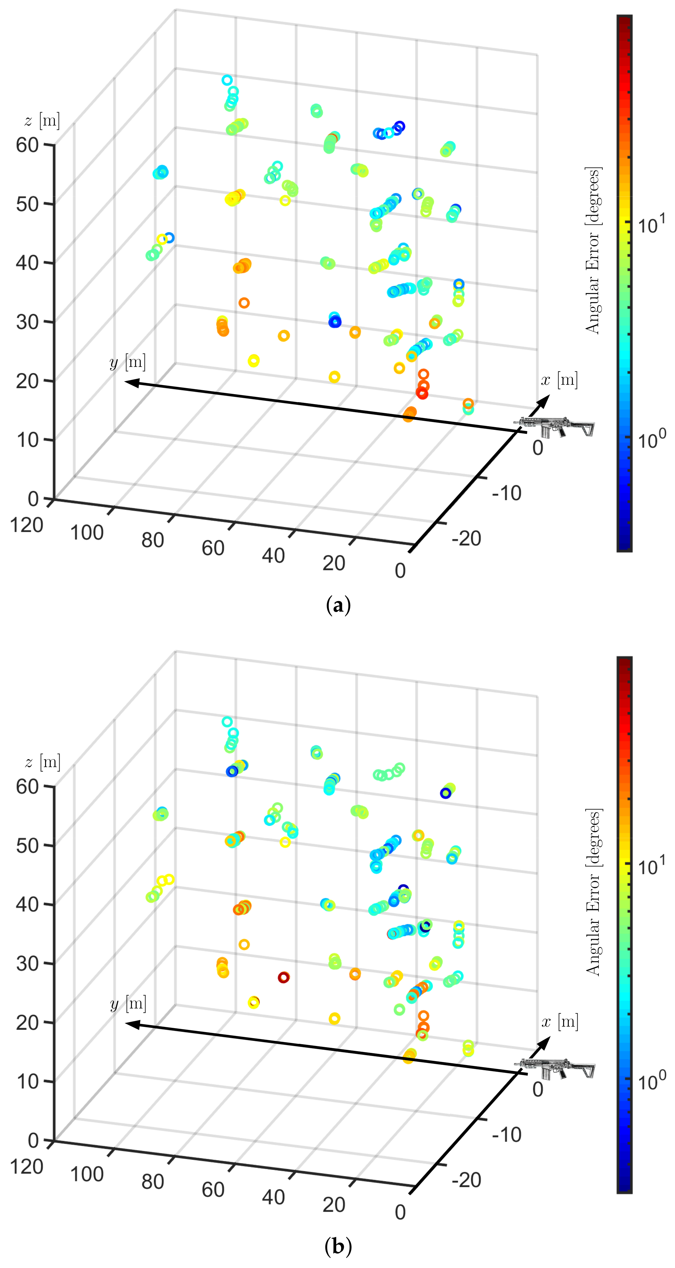
4.2. Field Recordings

The recordings were carried out in 5 sets. In the first one, 3 shoots were recorded only to make sure that the system was fully operational and were not used to evaluate its performance. The next four sets contain, respectively, 50, 50, 60, and 87 gunshot recordings. Summing up, we have a total of 250 gunshots, all from a Carbine IMBEL 7.62 IA2 [70]. In each series, the drone’s flight height varied from 8.8 m up to 60.5 m. The upper limit of flight height was set to ensure safety since the additional payload in the drone compromises its ability to withstand wind gusts. In some recordings, both muzzle blast and shockwave components are present, while in cases where the drone was not positioned in the propagation path of the shockwave, only the muzzle blast is present. In this work, we address DoA estimation of the muzzle blast only.
In order to avoid issues related to automatic detection, the system recorded continuously for the duration of the flight, and signals were clipped, manually preserving the muzzle blast only. These two acoustic signatures overlapped in a few recordings. When analysing the results, we found out that azimuth estimations were biased. The bias was similar in the third, fourth, and fifth sets but clearly different for the second run. This, combined with the fact that the UAV required a calibration of its magnetic sensor between the second and the third runs, indicates that this bias can be credited to electromagnetic interference in electronic compassed caused by other circuits aboard. As this bias was spotted only when processing the signals in the laboratory, the value of the compensation had to be estimated directly from the gunshots. To estimate the bias, we computed the mean azimuth error, but in order to mitigate the deleterious effects of possible outliers, we used only DoA estimations with zenith errors less than 3 ° . Finally, we obtained bias correction values of −8.6743 ° for the second set and −16.7746 ° for the third, fourth, and fifth sets.
The experiments were designed to evaluate the performed of the algorithms under different controlled values of SNR for the gunshot signals. However, other important measurements from GPS and attitude sensors are assumed to be inherently noisy. Table 4 presents the results obtained for the 247 muzzle blast gunshot signals under test. Although for the simulated signals we used as the hit rate the percentage of shots with angular errors lower than 3 ° , for the real gunshot signals, we increased this threshold to 10 ° . The results in Table 4 represent an average of the different recording conditions, depending on the position of the drone as shall be seen in the following.
Figure 8 illustrates the relationship between the position of the drone and the DoA estimation error. Notice that, as the distances between drone and shooter are not substantially large, 120 m at most, the error observed in this experiment is not strongly related to the distance but is rather correlated to relative position: when the drone is within a cone in front of the weapon, the results are poorer. We analyzed the recordings from positions within this cone and observed distorted signals in most of them. These positions are in the field of view of the shockwave but also in the direction of and in a small distance from the gun barrel. This suggests that the causes of the distortions are twofold: overlap of shockwave and muzzle blast components and a great signal intensity saturating the sensor. In an attempt to measure the system performance in better positioning, we took all gunshots recorded in a region outside a 35 ° cone open from the weapon muzzle and the error dropped considerably. The hit rate increased to 92.86% for the MBSS technique and to 95.54% for the LS + MF method instead of the former 72.87% and 70.45%, respectively.

5. Discussion and Conclusions

In this work, we analyze the problem of determining the position of a shooter based on gunshot signals acquired using a microphone array mounted on a multirotor UAV. We have conducted a comprehensive literature review on essential topics characterizing the state-of-the-art for this kind of application. We narrow down the focus on the main task, which is to determine the direction of arrival for the muzzle blast and to evaluate the performance of two well-established DoA estimation techniques as well as two important preprocessing methods.
We carry out extensive simulations to evaluate the performance of DoA algorithms and to tune their parameters before finally testing the methods with actual gunshot dates recorded in a firing range. Based on our experimental results, we claim that an aerial microphone array mounted on a drone can be used to obtain good estimates of gunshot direction of arrival using different techniques. The experiments also highlight the fact that the accuracy of the estimates are sensitive to the drone position relative to the shooter and emphasize that better results can be achieved with a system that can fly at higher altitudes, in which case it would be possible to estimate the position of the shooter as well.
Nevertheless, issues like detection, classification, and noise cancellation algorithms require further investigation, testing, and validation to achieve a fully functional, reliable, and autonomous system.

Author Contributions

Authors individual contributions are listed as follows. Conceptualization, J.A.A.J. and A.L.L.R.; data curation, F.G.S.; formal analysis, F.G.S.; funding acquisition, J.A.A.J. and A.L.L.R.; investigation, R.P.F., F.G.S., and J.A.A.J.; methodology, F.G.S. and J.A.A.J.; project administration, J.A.A.J.; resources, J.A.A.J. and A.L.L.R.; software, F.G.S.; supervision, J.A.A.J. and A.L.L.R.; validation, F.G.S.; visualization, F.G.S. and J.A.A.J.; writing—original draft preparation, F.G.S. and R.P.F.; writing—review and editing, J.A.A.J., A.L.L.R., F.G.S., and R.P.F.

Funding

This study was financed in part by the Brazilian Army, in part by the Coordenação de Aperfeiçoamento de Pessoal de Nível Superior—Brasil (CAPES), finance code n ° 23038.018065/2018-17, and in part by the Norwegian Agency for International Cooperation and Quality Enhancement in Higher Education (Diku), project number UTF-2018-CAPES-Diku/10002.

Acknowledgments

The authors would like to thank Jorge P. do Bomfim for his support in all audio recordings, drone setup, and operation. We would also like to thank the Brazilian Army Evaluation Center (CAEx) for the support in the recordings of real gunshot signals. CAEx provided highly skilled staff, location, gun, and ammunition.

Conflicts of Interest

The authors declare no conflict of interest. The funders had no role in the design of the study; in the collection, analyses, or interpretation of data; in the writing of the manuscript; or in the decision to publish the results.

Appendix A. Complete Simulation Results

Table A1. LS method simulation: complete results.
Without PreprocessingMedian FilterWiener Filter
SNR dB n/Window
Size (ms)
Mean
Error ( ° )
Standard
Deviation ( ° )
Error < 3 °
( % )
Mean
Error ( ° )
Standard
Deviation ( ° )
Error < 3 °
( % )
Mean
Error ( ° )
Standard
Deviation ( ° )
Error < 3 °
( % )
103/200.51053.926999.10000.32590.511099.300019.417429.260063.9667
3/350.41132.956999.33330.31660.489799.23337.516819.834885.4667
3/500.54984.317898.80000.31370.472099.33336.785918.875986.3667
4/200.35772.564899.43330.29560.456699.466714.278425.621067.2667
4/350.34562.586099.60000.29370.459899.33335.711617.166486.8000
4/500.44923.785999.53330.29830.465299.43334.909715.820288.4333
5/200.72664.265597.33330.25700.406599.600017.362723.831449.3333
5/350.64154.046597.90000.25880.415099.60007.296217.081277.1333
5/500.63434.161198.03330.25990.420699.60006.252815.960280.3000
6/203.86319.262379.70000.21550.411399.766720.903021.000631.3000
6/353.63648.780980.56670.21110.364199.800011.407617.044255.8333
6/503.61978.742380.30000.20810.355599.800010.156216.094659.5667
53/208.943821.772183.03330.45091.872498.766747.879427.955013.4000
3/359.039921.919382.93330.39800.605798.766735.885731.706633.7000
3/509.277221.974282.30000.47501.964498.133333.390931.634337.4333
4/206.304518.211885.93330.35580.552598.900043.640928.984815.2333
4/356.753218.976285.26670.36340.547498.866732.897431.285334.8000
4/506.699218.573784.96670.39601.015098.500030.449531.458839.6333
5/209.048618.064568.83330.35761.090198.886743.588726.25807.9333
5/358.970718.534569.13330.33060.703898.900033.116028.515123.4333
5/508.743317.727569.23330.37171.404398.833331.287928.812726.4667
6/2016.335517.795634.00000.96644.518196.166742.253422.59813.1000
6/3516.167217.680433.66670.66252.985896.966733.727923.519911.7333
6/5015.832517.401434.90000.93304.563196.566732.158423.762613.8333
23/2025.000231.269054.23331.20666.501595.966754.870023.42662.7333
3/3525.107131.275753.86671.20676.051696.033349.762927.401611.4333
3/5025.480731.200152.86671.38707.582495.366748.907627.998913.2667
4/2020.155528.847556.96670.87644.764596.766752.921723.93412.6333
4/3520.387329.089256.73330.88034.949496.733348.323828.155811.7333
4/5020.628329.048656.10000.90614.218396.233347.345928.530513.7667
5/2022.829625.808135.76671.43676.068693.666752.356922.89730.9667
5/3522.719226.222537.60001.49926.172393.466747.806226.47876.6000
5/5022.369525.716336.50001.87497.266892.200046.641727.08578.6667
6/2027.980820.998512.40004.695211.296880.100050.687521.53350.3667
6/3527.522821.090613.30004.499110.749879.800046.089423.39742.3000
6/5027.211120.688413.06675.606112.574977.466744.699423.93383.7000
03/2036.537231.977033.40003.869713.966689.800056.011422.11680.7667
3/3536.530631.865133.23333.728413.170088.233354.150724.30324.6333
3/5036.613631.920333.60005.754017.539884.966752.731125.05676.1333
4/2031.595831.228235.30003.649713.906189.200054.820922.33060.9000
4/3532.065331.425135.36673.586212.619187.966753.190424.87875.0667
4/5032.148131.525535.23335.339616.282683.933351.826225.77066.8000
5/2032.775327.804320.33335.826914.514377.233354.492121.74180.1333
5/3532.984327.826418.70006.162614.373375.200052.864323.98312.4000
5/5033.852128.158719.33337.485916.404972.533351.471424.81033.5667
6/2034.919522.26856.100011.673917.723556.800053.460021.16480.2333
6/3535.211122.21095.666712.720218.104352.566750.696422.52400.7000
6/5035.579022.40755.900013.946819.189850.166749.694422.58820.9333
−23/2045.141330.256819.200012.367526.075474.033356.625821.74860.1333
3/3545.909129.635617.733314.783028.475868.833356.185722.80851.6667
3/5045.660429.825418.366717.272130.477263.366755.817523.01732.2333
4/2042.271930.578419.166712.494025.059267.933355.880421.43360.1000
4/3542.754030.276217.766714.967127.477963.300055.601723.05521.9667
4/5042.711830.157117.600017.038328.842258.133355.097223.37922.4667
5/2042.486027.68018.866715.759923.622751.566755.541921.44170.0667
5/3542.646127.30378.366717.856425.171046.100054.961622.80000.9000
5/5043.137127.22148.200019.790725.976641.566754.740723.07731.0667
6/2042.316523.03142.533322.901323.637230.600054.871721.03240.1333
6/3542.604323.02152.133324.521323.938826.733353.422122.05510.2333
6/5042.674723.05242.433326.486924.345824.300053.217622.32570.3000
−33/2048.950328.009212.466720.076732.146359.533356.573321.76650.1667
3/3549.283728.351613.066723.463234.291555.100056.626722.11721.0000
3/5049.329028.312612.600026.506835.684349.100056.196622.52021.4333
4/2047.145128.578111.900019.772431.002553.933356.292821.44320.1333
4/3546.788028.819812.600022.969032.641749.700056.438622.32541.1000
4/5047.400528.484211.500026.241633.831243.366755.905122.74391.3333
5/2046.726926.27935.200022.295627.351138.300056.007321.21510.1333
5/3546.393626.57455.766725.108429.195434.566756.149722.06780.5667
5/5046.990426.56225.700028.220230.065930.066755.494922.43930.6000
6/2045.907322.86741.133328.528224.719021.066755.475221.05320.1333
6/3545.738322.99031.300031.070225.838118.233354.811222.02720.2333
6/5046.316423.21091.166732.934625.687015.766754.283021.96270.2667
Table A2. MBSS simulation: complete results.
Without PreprocessingMedian FilterWiener Filter
SNR dB Window Size /
Frame Size (ms)
Mean
Error ( ° )
Standard
Deviation ( ° )
Error < 3 °
( % )
Mean
Error ( ° )
Standard
Deviation ( ° )
Error < 3 °
( % )
Mean
Error ( ° )
Standard
Deviation ( ° )
Error < 3 °
( % )
1025/ 100.45310.446899.30000.52750.602998.43333.176710.744790.8000
35/100.45010.432899.30000.52200.589698.53338.946120.377180.2000
35/120.44730.425999.36670.50940.556398.66672.20188.020592.9667
50/100.45240.433899.33330.53540.617298.233311.453523.474177.0000
50/120.44150.408499.40000.49560.530198.73333.378111.663191.3000
50/150.44150.408499.40000.49560.530198.73333.378111.663191.3000
50/200.44150.408499.40000.49560.530198.73333.378111.663191.3000
525/ 100.51080.539298.93330.60130.711197.733320.935028.610755.7333
35/100.50690.539398.86670.60150.701997.866731.975331.945939.9667
35/120.48650.493499.06670.55740.624098.233316.810326.650363.3667
50/100.49850.510099.03330.59430.690797.766736.238931.732733.5667
50/120.46080.450699.16670.51670.562498.666723.515429.745552.9000
50/150.46080.450699.16670.51670.562498.666723.515429.745552.9000
50/200.46080.450699.16670.51670.562498.666723.515429.745552.9000
225/ 100.65871.005197.10000.74380.968996.100040.442131.561723.8333
35/100.67602.358897.26670.84663.270296.133346.939630.938416.6333
35/120.58970.724697.96670.68310.832897.033336.638832.288829.8000
50/100.65111.588597.56670.84263.249996.600050.031528.405211.7667
50/120.50970.540898.70000.57690.656398.300042.387731.830922.3000
50/150.50970.540898.70000.57690.656398.300042.387731.830922.3000
50/200.50970.540898.70000.57690.656398.300042.387731.830922.3000
025/ 100.81221.954495.90001.26825.415893.733348.312329.813812.0667
35/101.18275.833795.40001.63288.018593.466752.349227.86957.3000
35/120.70210.846896.50000.87221.526495.166745.605230.625215.4000
50/100.85042.512695.76671.17904.365093.766753.143226.89286.5000
50/120.58710.707297.66670.80103.415896.566748.869230.105812.2333
50/150.58710.707297.66670.80103.415896.566748.869230.105812.2333
50/200.58710.707297.66670.80103.415896.566748.869230.105812.2333
−225/ 101.90499.178192.10003.630914.108288.333353.383427.62595.0333
35/102.223010.123491.96674.637016.570186.666755.502026.48143.5000
35/120.95772.858694.53331.74327.363591.400051.709529.12087.5333
50/101.86689.285893.40003.459214.069289.300055.218225.26052.9333
50/120.67880.869096.73331.20455.629694.666753.476927.67945.8000
50/150.67880.869096.73331.20455.629694.666753.476927.67945.8000
50/200.67880.869096.73331.20455.629694.666753.476927.67945.8000
−325/ 102.785712.165690.66676.766420.368182.966754.279427.45134.6667
35/103.486313.878489.66678.375522.422880.200056.070025.90852.4000
35/121.33765.684392.86673.508514.016287.466752.800128.50945.8333
50/102.634411.697291.80006.283620.045384.733356.567424.88492.2333
50/120.97514.424095.93332.01949.422092.366754.900027.07544.2667
50/150.97514.424095.93332.01949.422092.366754.900027.07544.2667
50/200.97514.424095.93332.01949.422092.366754.900027.07544.2667
−525/ 108.999523.779178.300017.898532.596962.900055.568626.82712.1333
35/1012.111127.974274.633322.277935.484159.033357.170326.12661.1000
35/124.499815.666884.300012.664028.445369.900054.997327.97553.2667
50/108.530223.374580.300019.030733.828764.866756.828124.41910.9000
50/123.057613.038390.73339.198124.120978.933356.341927.03531.8667
50/153.057613.038390.73339.198124.120978.933356.341927.03531.8667
50/203.057613.038390.73339.198124.120978.933356.341927.03531.8667
−825/ 1033.531139.817741.233344.303540.991726.633357.201226.89901.8000
35/1036.334539.972438.066746.846641.095626.000057.518225.59220.8667
35/1221.741634.773553.666735.280540.214835.566756.528927.84572.1667
50/1034.008239.606443.400046.591240.833725.933357.752024.72070.6667
50/1218.842433.586061.900034.436540.566140.200057.258026.39921.7000
50/1518.842433.586061.900034.436540.566140.200057.258026.39921.7000
50/2018.842433.586061.900034.436540.566140.200057.258026.39921.7000

References

  1. Dong, J.; Wu, G.; Yang, T.; Jiang, Z. Battlefield situation awareness and networking based on agent distributed computing. Phys. Commun. 2019, 33, 178–186. [Google Scholar] [CrossRef]
  2. Astapov, S.; Berdnikova, J.; Ehala, J.; Kaugerand, J.; Preden, J.S. Gunshot acoustic event identification and shooter localization in a WSN of asynchronous multichannel acoustic ground sensors. Multidimens. Syst. Signal Process. 2018, 29, 563–595. [Google Scholar] [CrossRef]
  3. Ramos, A.L.L. Acoustic Sniper Positioning Systems. Ph.D. Thesis, University of Oslo, Oslo, Norway, 2015. [Google Scholar]
  4. Kastek, M.; Dulski, R.; Trzaskawka, P.; Piątkowski, T.; Polakowski, H. Spectral measurements of muzzle flash with multispectral and hyperspectral sensor. In International Symposium on Photoelectronic Detection and Imaging 2011: Advances in Infrared Imaging and Applications; International Society for Optics and Photonics: Bellingham, WA, USA, 2011; Volume 8193, p. 81933Y. [Google Scholar]
  5. Borzino, A.M.C.R.; Apolinário, J.A., Jr.; de Campos, M.L.R.; Biscainho, L.W.P. Signal enhancement for gunshot DOA estimation with median filters. In Proceedings of the 6th Latin American Symposium on Circuits & Systems (LASCAS), Montevideo, Uruguay, 24–27 February 2015. [Google Scholar]
  6. Borzino, A.M.C.R.; Apolinário, J.A., Jr.; de Campos, M.L.R. Consistent DOA estimation of heavily noisy gunshot signals using a microphone array. IET Radar Sonar Navig. 2016, 10, 1519–1527. [Google Scholar] [CrossRef]
  7. Borzino, A.M.C.R.; Apolinário, J.A., Jr.; de Campos, M.L.R. Robust DOA estimation of heavily noisy gunshot signals. In Proceedings of the International Conference on Acoustics, Speech and Signal Processing (ICASSP), South Brisbane, QLD, Australia, 19–24 April 2015; pp. 449–453. [Google Scholar]
  8. Ntalampiras, S. Moving vehicle classification using wireless acoustic sensor networks. IEEE Trans. Emerg. Top. Comput. Intell. 2018, 2, 129–138. [Google Scholar] [CrossRef]
  9. Prince, P.; Hill, A.; Piña Covarrubias, E.; Doncaster, P.; Snaddon, J.L.; Rogers, A. Deploying Acoustic Detection Algorithms on Low-Cost, Open-Source Acoustic Sensors for Environmental Monitoring. Sensors 2019, 19, 553. [Google Scholar] [CrossRef] [PubMed]
  10. Prasad, R. Alexa Everywhere: AI for Daily Convenience. In Proceedings of the Twelfth ACM International Conference on Web Search and Data Mining, Melbourne, VIC, Australia, 11–15 February 2019. [Google Scholar]
  11. Sibanyoni, S.V.; Ramotsoela, D.T.; Silva, B.J.; Hancke, G.P. A 2-D Acoustic Source Localization System for Drones in Search and Rescue Missions. IEEE Sens. J. 2019, 19, 332–341. [Google Scholar] [CrossRef]
  12. Hoshiba, K.; Washizaki, K.; Wakabayashi, M.; Ishiki, T.; Kumon, M.; Bando, Y.; Gabriel, D.; Nakadai, K.; Okuno, H. Design of UAV-embedded microphone array system for sound source localization in outdoor environments. Sensors 2017, 17, 2535. [Google Scholar] [CrossRef]
  13. Schmidt, R.O. Multiple emitter location and signal parameter estimation. IEEE Trans. Antennas Propag. 1986, 34, 276–280. [Google Scholar] [CrossRef] [Green Version]
  14. Nakamura, K.; Nakadai, K.; Asano, F.; Hasegawa, Y.; Tsujino, H. Intelligent sound source localization for dynamic environments. In Proceedings of the International Conference on Intelligent Robots and Systems (IROS), St. Louis, MI, USA, 10–15 October 2009; pp. 664–669. [Google Scholar]
  15. Nakamura, K.; Nakadai, K.; Asano, F.; Ince, G. Intelligent sound source localization and its application to multimodal human tracking. In Proceedings of the International Conference on Intelligent Robots and Systems (IROS), Francisco, CA, USA, 25–30 September 2011; pp. 143–148. [Google Scholar]
  16. Okutani, K.; Yoshida, T.; Nakamura, K.; Nakadai, K. Outdoor auditory scene analysis using a moving microphone array embedded in a quadrocopter. In Proceedings of the International Conference on Intelligent Robots and Systems (IROS), Algarve, Portugal, 7–12 October 2012; pp. 3288–3293. [Google Scholar]
  17. Furukawa, K.; Okutani, K.; Nagira, K.; Otsuka, T.; Itoyama, K.; Nakadai, K.; Okuno, H.G. Noise correlation matrix estimation for improving sound source localization by multirotor UAV. In Proceedings of the International Conference on Intelligent Robots and Systems (IROS), Tokyo, Japan, 3–7 November 2013; pp. 3943–3948. [Google Scholar]
  18. Ohata, T.; Nakamura, K.; Mizumoto, T.; Taiki, T.; Nakadai, K. Improvement in outdoor sound source detection using a quadrotor-embedded microphone array. In Proceedings of the International Conference on Intelligent Robots and Systems (IROS), Daejeon, Korea, 9–14 October 2014; pp. 1902–1907. [Google Scholar]
  19. Wang, L.; Cavallaro, A. Time-frequency processing for sound source localization from a micro aerial vehicle. In Proceedings of the International Conference on Acoustics, Speech and Signal Processing (ICASSP), New Orleans, LA, USA, 5–9 March 2017; pp. 496–500. [Google Scholar]
  20. Wang, L.; Cavallaro, A. Acoustic sensing from a multi-rotor drone. Sens. J. 2018, 18, 4570–4582. [Google Scholar] [CrossRef]
  21. Wang, L.; Cavallaro, A. Ear in the sky: Ego-noise reduction for auditory micro aerial vehicles. In Proceedings of the 13th International Conference on Advanced Video and Signal Based Surveillance (AVSS), Colorado Springs, CO, USA, 23–26 August 2016; pp. 152–158. [Google Scholar]
  22. Basiri, M.; Schill, F.; Lima, P.; Floreano, D. On-board relative bearing estimation for teams of drones using sound. IEEE Robot. Autom. Lett. 2016, 1, 820–827. [Google Scholar] [CrossRef]
  23. Wang, L.; Sanchez-Matilla, R.; Cavallaro, A. Tracking a moving sound source from a multi-rotor drone. In Proceedings of the International Conference on Intelligent Robots and Systems (IROS), Madrid, Spain, 1–5 October 2018; pp. 2511–2516. [Google Scholar]
  24. Calderon, D.M.P.; Apolinário, J.A., Jr. Shooter localization based on DoA estimation of gunshot signals and digital map information. Lat. Am. Trans. 2015, 13, 441–447. [Google Scholar] [CrossRef]
  25. Fernandes, R.P.; Borzino, A.M.C.R.; Ramos, A.L.L.; Apolinário, J.A., Jr. Investigating the potential of UAV for gunshot DoA estimation and shooter localization. In Proceedings of the Simpósio Brasileiro de Telecomunicações e Processamento de Sinais, Belém, Brazil, 30 August–2 September 2016. [Google Scholar]
  26. Fernandes, R.P.; Ramos, A.L.L.; Apolinário, J.A., Jr. Airborne DoA estimation of gunshot acoustic signals using drones with application to sniper localization systems. In Proceedings of the SPIE Defense, Security, and Sensing, Anaheim, CA, USA, 9–13 April 2017. [Google Scholar]
  27. Beck, S.D.; Nakasone, H.; Marr, K.W. An introduction to forensic gunshot acoustics. In Proceedings of the 162nd Meeting of the Acoustical Society of America, San Diego, CA, USA, 31 October–4 November 2011. [Google Scholar]
  28. Brustad, B.M.; Freytag, J.C. A survey of audio forensic gunshot investigations. In Proceedings of the 26th International Conference: Audio Forensics in the Digital Age, Denver, CO, USA, 7–9 July 2005. [Google Scholar]
  29. Beck, S.D.; Nakasone, H.; Marr, K.W. Variations in recorded acoustic gunshot waveforms generated by small firearms. J. Acoust. Soc. Am. 2011, 129, 1748–1759. [Google Scholar] [CrossRef] [PubMed]
  30. Routh, T.K.; Maher, R.C. Recording anechoic gunshot waveforms of several firearms at 500 kilohertz sampling rate. In Proceedings of the 171st Meeting of the Acoustical Society of America, Salt Lake City, UT, USA, 23–27 May 2016. [Google Scholar]
  31. Maher, R.C. Modeling and Signal Processing of Acoustic Gunshot Recordings. In Proceedings of the IEEE 12th Digital Signal Processing Workshop & 4th IEEE Signal Processing Education Workshop, Teton National Park, WY, USA, 24–27 September 2006; pp. 257–261. [Google Scholar]
  32. Maher, R.C. Acoustical Characterization of Gunshots. In Proceedings of the IEEE Workshop on Signal Processing Applications for Public Security and Forensics, Washington, DC, USA, 11–13 April 2007. [Google Scholar]
  33. DuMond, J.W.; Cohen, E.R.; Panofsky, W.; Deeds, E. A determination of the wave forms and laws of propagation and dissipation of ballistic shock waves. J. Acoust. Soc. Am. 1946, 18, 97–118. [Google Scholar] [CrossRef]
  34. George, J.; Kaplan, L.M. Shooter Localization using a Wireless Sensor Network of Soldier-Worn Gunfire Detection Systems. J. Adv. Inf. Fusion 2013, 8, 15–32. [Google Scholar]
  35. Ishiki, T.; Kumon, M. A microphone array configuration for an auditory quadrotor helicopter system. In Proceedings of the International Symposium on Safety, Security, and Rescue Robotics, Hokkaido, Japan, 27–30 October 2014. [Google Scholar]
  36. Strauss, M.; Mordel, P.; Miguet, V.; Deleforge, A. DREGON: Dataset and Methods for UAV-Embedded Sound Source Localization. In Proceedings of the International Conference on Intelligent Robots and Systems (IROS), Madrid, Spain, 1–5 October 2018. [Google Scholar]
  37. Scalart, P.; Liu, M. Wiener Filter for Noise Reduction and Speech Enhancement. Available online: https://www.mathworks.com/matlabcentral/fileexchange/24462-wiener-filter-for-noise-reduction-and-speech-enhancement (accessed on 12 January 2019).
  38. Plapous, C.; Marro, C.; Scalart, P. Improved signal-to-noise ratio estimation for speech enhancement. IEEE Trans. Audio Speech Lang. Process. 2006, 14, 2098–2108. [Google Scholar] [CrossRef]
  39. Ephraim, Y.; Malah, D. Speech enhancement using a minimum-mean square error short-time spectral amplitude estimator. IEEE Trans. Acoust. Speech Signal Process. 1984, 32, 1109–1121. [Google Scholar] [CrossRef] [Green Version]
  40. Fitzgerald, D. Harmonic/percussive separation using median filtering. In Proceedings of the 13th International Conference on Digital Audio Effects (DAFX10), Graz, Austria, 6–10 September 2010. [Google Scholar]
  41. Mäkinen, T.; Pertilä, P. Shooter localization and bullet trajectory, caliber, and speed estimation based on detected firing sounds. Appl. Acoust. 2010, 71, 902–913. [Google Scholar] [CrossRef]
  42. Hainsworth, S. Beat tracking and musical metre analysis. In Signal Processing Methods for Music Transcription; Springer: Berlin/Heidelberg, Germany, 2006; pp. 101–129. [Google Scholar]
  43. Chacon-Rodriguez, A.; Julian, P.; Castro, L.; Alvarado, P.; Hernández, N. Evaluation of gunshot detection algorithms. IEEE Trans. Circuits Syst. I Regul. Pap. 2010, 58, 363–373. [Google Scholar] [CrossRef]
  44. Freire, I.L.; Apolinário, J.A., Jr. Gunshot detection in noisy environment. In Proceeding of the 7th International Telecommunications Symposium, Manaus, Brazil, 7–9 September 2010. [Google Scholar]
  45. Ahmed, T.; Uppal, M.; Muhammad, A. Improving efficiency and reliability of gunshot detection systems. In Proceeding of the 2013 IEEE International Conference on Acoustics, Speech and Signal Processing, Vancouver, BC, Canada, 26–30 May 2013. [Google Scholar]
  46. Libal, U.; Spyra, K. Wavelet based shock wave and muzzle blast classification for different supersonic projectiles. Expert Syst. Appl. 2014, 41, 5097–5104. [Google Scholar] [CrossRef]
  47. Blandin, C.; Ozerov, A.; Vincent, E. Multi-source TDOA estimation in reverberant audio using angular spectra and clustering. Signal Process. 2012, 92, 1950–1960. [Google Scholar] [CrossRef] [Green Version]
  48. Van Trees, H.L. Optimum Array Processing—Part IV—Detection, Estimation, and Modulation Theory, Optimum Array Processing; John Wiley & Sons: Hoboken, NJ, USA, 2004. [Google Scholar]
  49. Knapp, C.H.; Carter, G.C. The generalized correlation method for estimation of time delay. IEEE Trans. Acoust. Speech Signal Process. 1976, 24, 320–327. [Google Scholar] [CrossRef] [Green Version]
  50. Van Den Broeck, B.; Bertrand, A.; Karsmakers, P.; Vanrumste, B.; Moonen, M. Time-domain generalized cross correlation phase transform sound source localization for small microphone arrays. In Proceeding of the 5th European DSP Education and Research Conference (EDERC), Amsterdam, The Netherlands, 13–14 September 2012; pp. 76–80. [Google Scholar]
  51. Ribeiro, J.G.; Serrenho, F.G.; Apolinário, J.A., Jr.; Ramos, A.L.L. Effective direction of arrival estimation of gunshot signals from an in-flight unmanned aerial vehicle. Autom. Target Recognit. XXVIII 2018, 10648, 106480H. [Google Scholar]
  52. Qin, B.; Zhang, H.; Fu, Q.; Yan, Y. Subsample time delay estimation via improved GCC PHAT algorithm. In Proceedings of the 9th International Conference on Signal Processing, Beijing, China, 26–29 October 2008; pp. 2579–2582. [Google Scholar]
  53. Brandstein, M.; Silverman, H. A robust method for speech signal time-delay estimation in reverberant rooms. In Proceedings of the International Conference on Acoustics, Speech, and Signal Processing (ICASSP), Munich, Germany, 21–24 April 1997. [Google Scholar]
  54. Freire, I.L.; Apolinário, J.A., Jr. DoA of gunshot signals in a spatial microphone array: Performance of the interpolated Generalized Cross-Correlation method. In Proceedings of the 6th Argentine School of Micro-Nanoelectronics, Technology and Applications (EAMTA), Buenos Aires, Argentina, 11–12 August 2011. [Google Scholar]
  55. Ribeiro, J.G.C.; Serrenho, F.G.; Apolinário, J.A., Jr.; Ramos, A.L.L. Improved DoA estimation with application to bearings-only acoustic source localization. In Proceedings of the International Symposium on Signal Processing and Information Technology (ISSPIT), Bilbao, Spain, 8–20 December 2017; pp. 100–105. [Google Scholar]
  56. Lebarbenchon, R.; Camberlein, E. Multi-Channel BSS Locate. Available online: http://bass-db.gforge.inria.fr/bss_locate/ (accessed on 20 February 2018).
  57. Loesch, B.; Yang, B. Adaptive segmentation and separation of determined convolutive mixtures under dynamic conditions. In International Conference on Latent Variable Analysis and Signal Separation; Springer: Berlin/Heidelberg, Germany, 2010; pp. 41–48. [Google Scholar]
  58. Nesta, F.; Svaizer, P.; Omologo, M. Cumulative state coherence transform for a robust two-channel multiple source localization. In International Conference on Independent Component Analysis and Signal Separation; Springer: Berlin/Heidelberg, Germany, 2009; pp. 290–297. [Google Scholar]
  59. Yamaoka, K.; Ono, N.; Makino, S.; Yamada, T. Time-frequency-bin-wise Switching of Minimum Variance Distortionless Response Beamformer for Underdetermined Situations. In Proceedings of the International Conference on Acoustics, Speech and Signal Processing (ICASSP), Brighton, UK, 12–17 May 2019; pp. 7908–7912. [Google Scholar]
  60. McCowan, I.; Lincoln, M.; Himawan, I. Microphone array shape calibration in diffuse noise fields. Trans. Audio Speech Lang. Process. 2008, 16, 666–670. [Google Scholar] [CrossRef]
  61. Doğançay, K. Bearings-only target localization using total least squares. Signal Process. 2005, 85, 1695–1710. [Google Scholar] [CrossRef]
  62. Freire, I.L.; Apolinário, J.A., Jr. Localização de atirador por arranjo de microfones (in Portuguese). SBAI 2011, X, 1049–1053. [Google Scholar]
  63. Barger, J.E.; Milligan, S.D.; Brinn, M.S.; Mullen, R.J. Systems and Methods for Determining Shooter Locations with Weak Muzzle Detection. U.S. Patent 7710828B2, 4 May 2010. [Google Scholar]
  64. DJI. Phantom 4 Specs. Available online: https://www.dji.com/phantom-4/info#specs (accessed on 13 April 2019).
  65. Google. Google Maps, Map Data: Google. Available online: https://www.google.com/maps/ (accessed on 6 August 2019).
  66. TASCAM. Handheld Recorder DR-40. Available online: https://tascam.com/us/product/dr-40/spec (accessed on 13 April 2019).
  67. Airdata UAV. Available online: https://airdata.com (accessed on 20 June 2019).
  68. DJI. Flight Control. Available online: https://developer.dji.com/mobile-sdk/documentation/introduction/flightController_concepts.html (accessed on 14 April 2018).
  69. Rorres, C.; Anton, H. Elementary Linear Algebra: Applications Version, 10th ed.; Wiley: Hoboken, NJ, USA, 2010. [Google Scholar]
  70. Indústria de Material Bélico do Brasil—IMBEL. Available online: http://www.imbel.gov.br/ (accessed on 7 July 2019).
Figure 1. Components of a gunshot signal: shockwave (left) and muzzle blast (right) of a caliber 7.62 mm rifle and the corresponding spectrogram.
Sensors 19 04271 g001
Figure 2. Azimuth ( ϕ ) and zenith ( θ ) relative to the center of the array: The x axis is oriented to the front of the drone, and the z axis points upwards.
Sensors 19 04271 g002
Figure 3. Effect of interpolation in generalized cross-correlation (GCC)-phase transform (PHAT): Note that r ^ x i x j ( τ ) is the GCC-PHAT without interpolation.
Sensors 19 04271 g003
Figure 4. Direction of arrival (DoA) calculation in a 2-D scenario.
Sensors 19 04271 g004
Figure 5. Drone used in the experiments: (a) landed; (b) during flight.
Sensors 19 04271 g005
Figure 6. Shooting site: In red (marker) is shooter location, and in blue is the allowed flight zone of the drone. Adapted from Google Maps [65].
Sensors 19 04271 g006
Figure 7. Attitude angles as measured by DJI Phantom 4, adapted from [68].
Sensors 19 04271 g007
Figure 8. Positions of the drone and respective DoA angular errors: Note that the greater errors (warmer colors) correspond to a region in front of the muzzle. (a) Results of the Least Squares method with median filtering. (b) Results of the MBSS method without preprocessing.
Sensors 19 04271 g008
Table 1. Planar array coordinates.
Microphonex (cm)y (cm)
126.5 25.5
226.527.0
3 25.0 26.0
4 25.0 25.5
Table 2. Least squares (LS) method simulation: The best parameters per signal-to-noise ratio (SNR).
Without PreprocessingMedian FilterWiener Filter
SNR dB n/Window
Size (ms)
Error < 3 ° (%)n/Window
Size (ms)
Error < 3 ° (%)n/Window
Size (ms)
Error < 3 ° (%)
104/3599.60006/5099.80004/5088.4333
54/2085.93334/2098.90004/5039.6333
24/2056.96674/2096.76674/5013.7667
04/3535.36673/2089.80004/506.8000
−23/2019.20003/2074.03334/502.4667
−33/3513.06673/2059.53333/501.4333
Table 3. Multi-channel Blind Source Separation (MBSS) Simulation: The best parameters per SNR.
Without PreprocessingMedian FilterWiener Filter
SNR dB Window Size/
Frame Size (ms)
Error < 3 ° [%]Window Size/
Frame Size (ms)
Error < 3 ° [%]Window Size/
Frame Size (ms)
Error < 3 ° [%]
1050/12
50/15
50/20
99.400050/12
50/15
50/20
98.733335/1292.9667
550/12
50/15
50/20
99.166750/12
50/15
50/20
98.666735/1263.3667
250/12
50/15
50/20
98.700050/12
50/15
50/20
98.300035/1229.8000
050/12
50/15
50/20
97.666750/12
50/15
50/20
96.566735/1215.4000
−250/12
50/15
50/20
96.733350/12
50/15
50/20
94.666735/127.5333
−350/12
50/15
50/20
95.933350/12
50/15
50/20
92.366735/125.8333
−550/12
50/15
50/20
90.733350/12
50/15
50/20
78.933335/123.2667
−850/12
50/15
50/20
61.900050/12
50/15
50/20
40.200035/122.1667
Table 4. Experimental data of muzzle blast DoA estimation.
Mean Error ( ° )Standard Deviaton ( ° )Error < 10 ° (%)
LS + MF8.38237.221570.4453
MBSS9.645112.211372.8745

