Indoor Crowd 3D Localization in Big Buildings from Wi-Fi Access Anonymous Data


Abstract
1. Introduction
1.1. Crowd Detection Approaches
1.1.1. General Artificial Vision Approach
1.1.2. Optical Anonymous Sensors
1.1.3. Sensor Networks
1.1.4. Wi-Fi Based Approaches
1.2. Description of Proposed System
1.2.1. Computational Methods
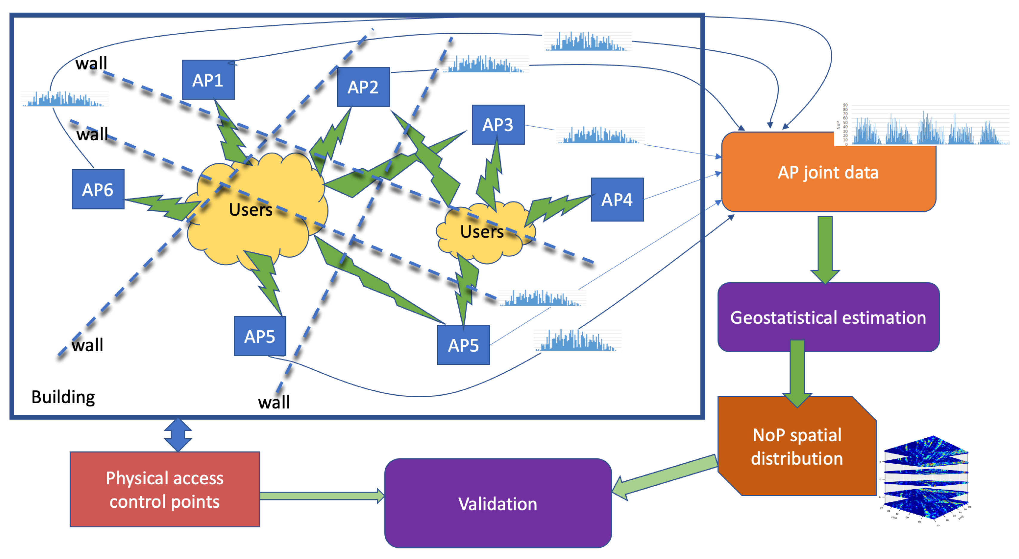
1.2.2. Intuitive Description of Our Approach
1.2.3. Software Resources
1.3. Paper Content
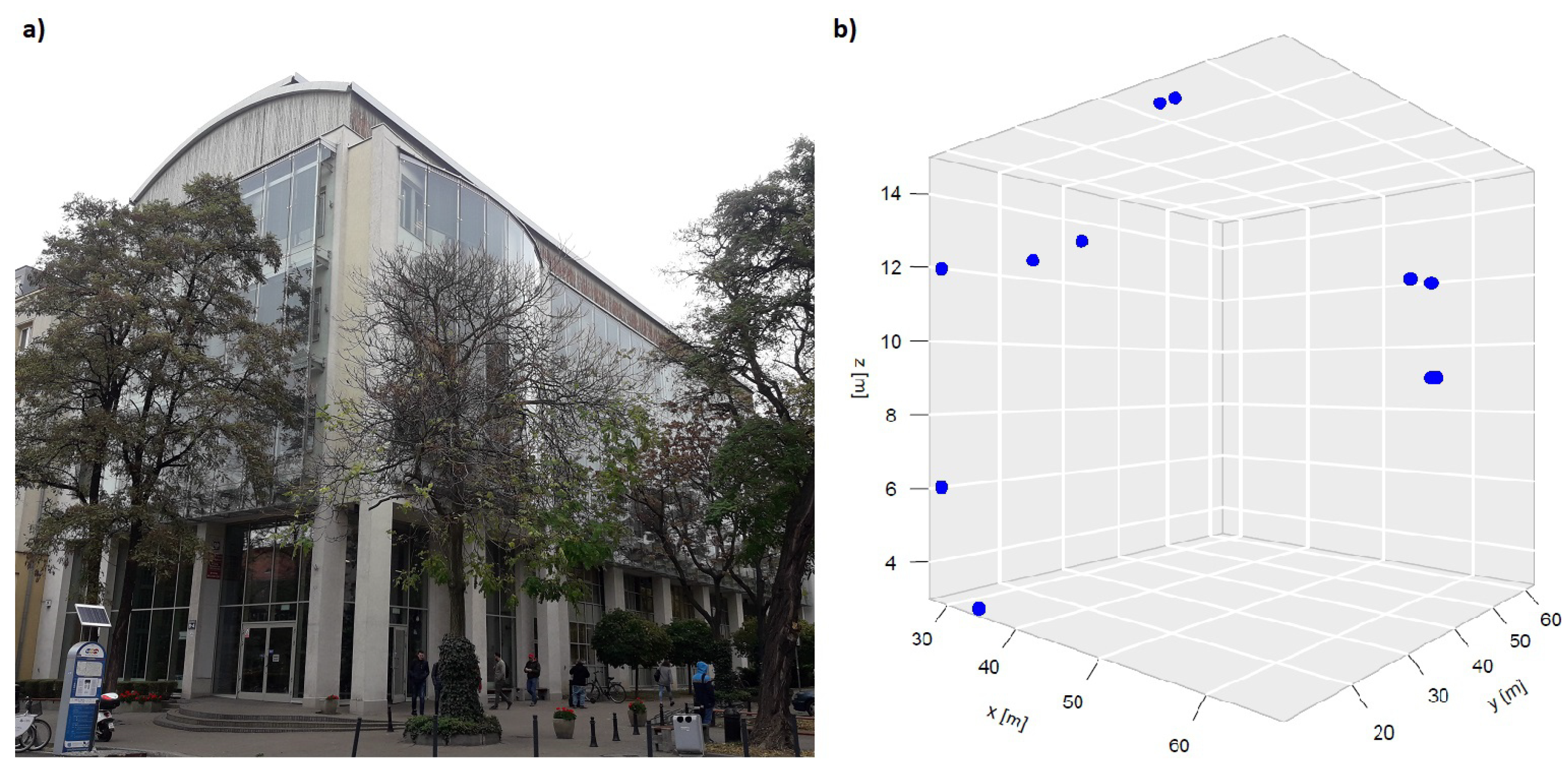
2. Experimental Data Gathering
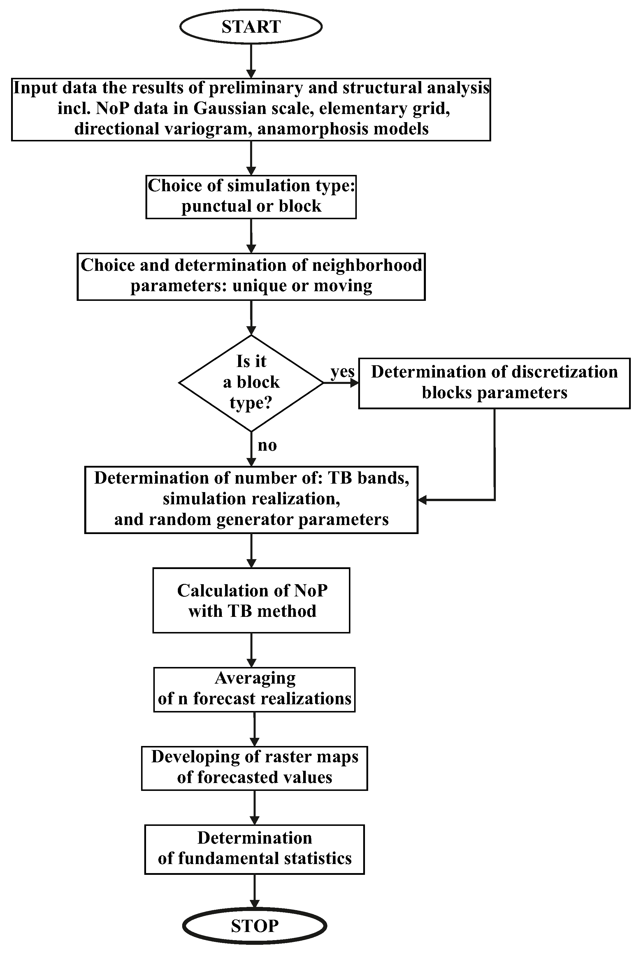
3. Spatial Estimation Mathematical Methods
- Preparation of the database according to input restrictions.
- Calculating fundamental statistics and assessing the Gaussianity of the input data.
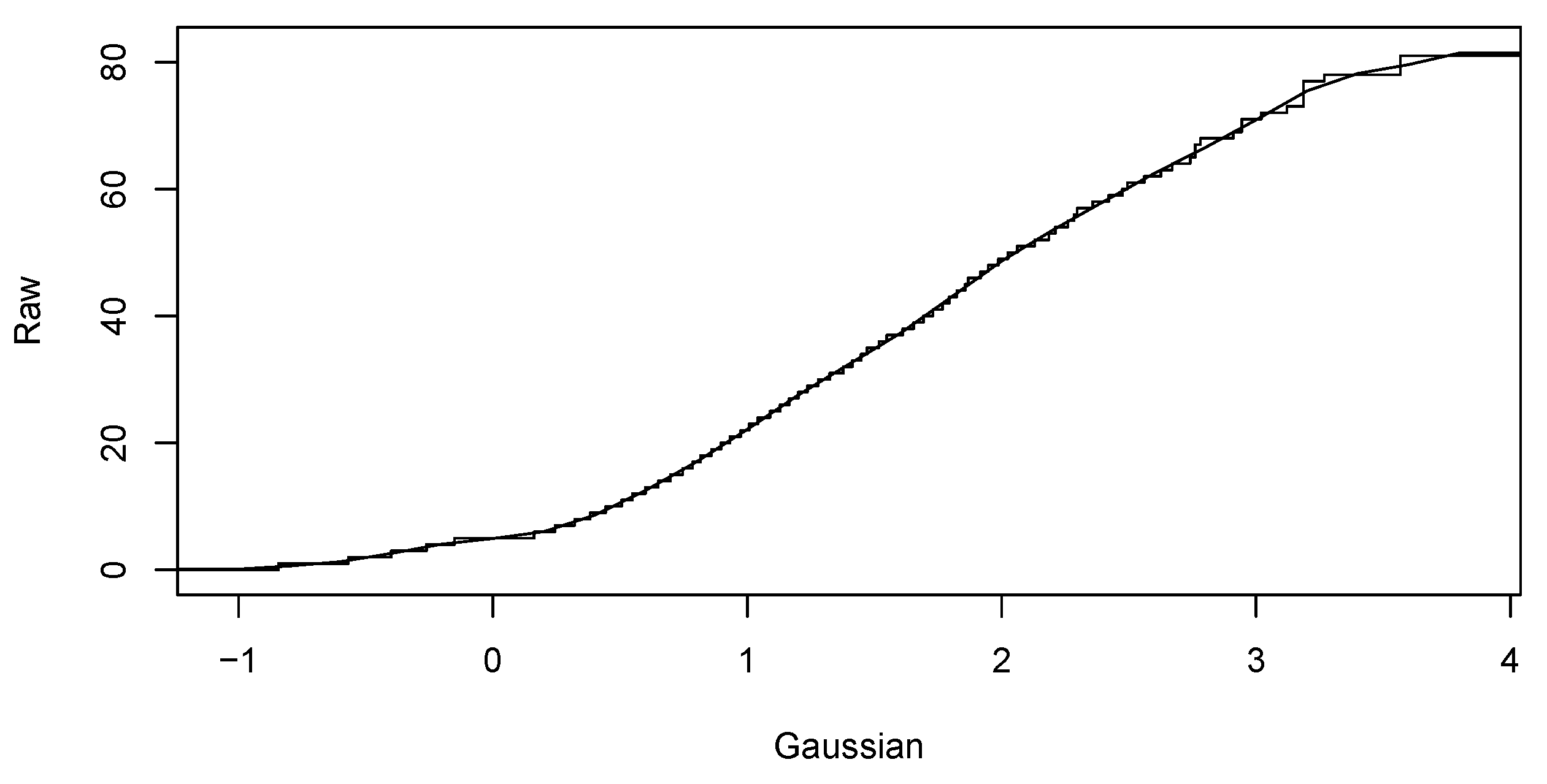
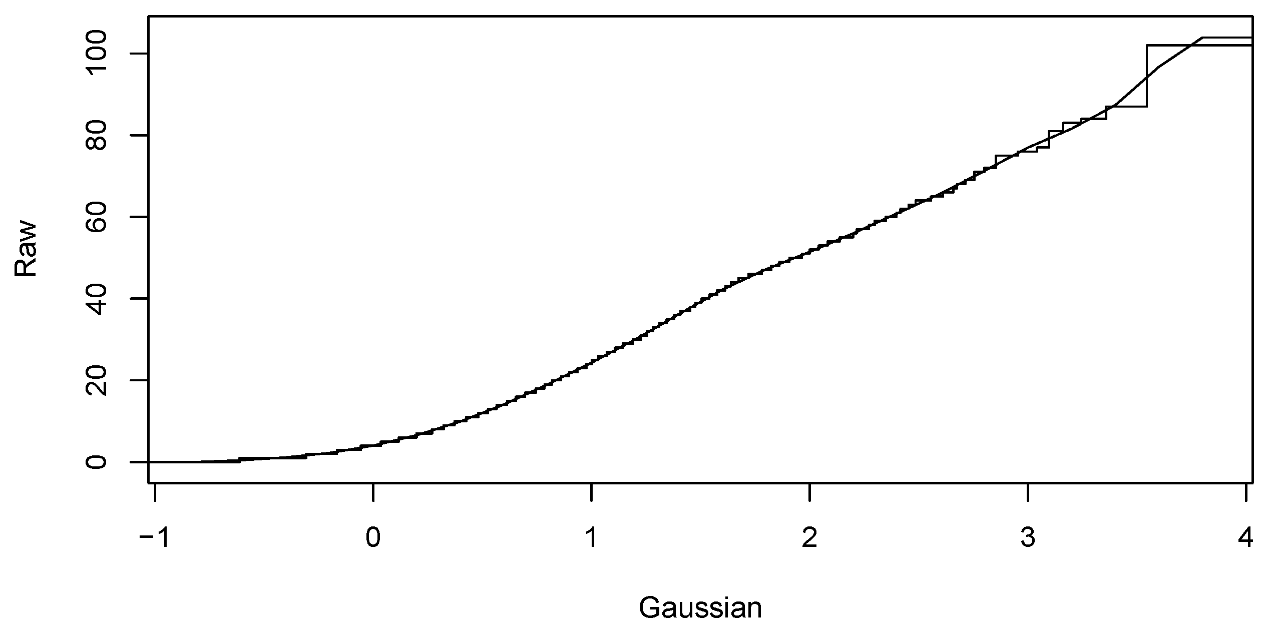
- Computing Gaussian anamorphosis on the raw data [43,44] to transform the input data into Gaussian distributed data. Computations were carried out using 100 Hermite polynomials for each year. The upper interval for 2016 indicates a wider expansion of the raw data. Finally, the anamorphosis result will be used in the random diagram of the Gaussian curve to obtain a random graph of the original variable. Graphs of Gaussian anamorphosis for the data collected each year are presented in Figure 9 and Figure 10, respectively.
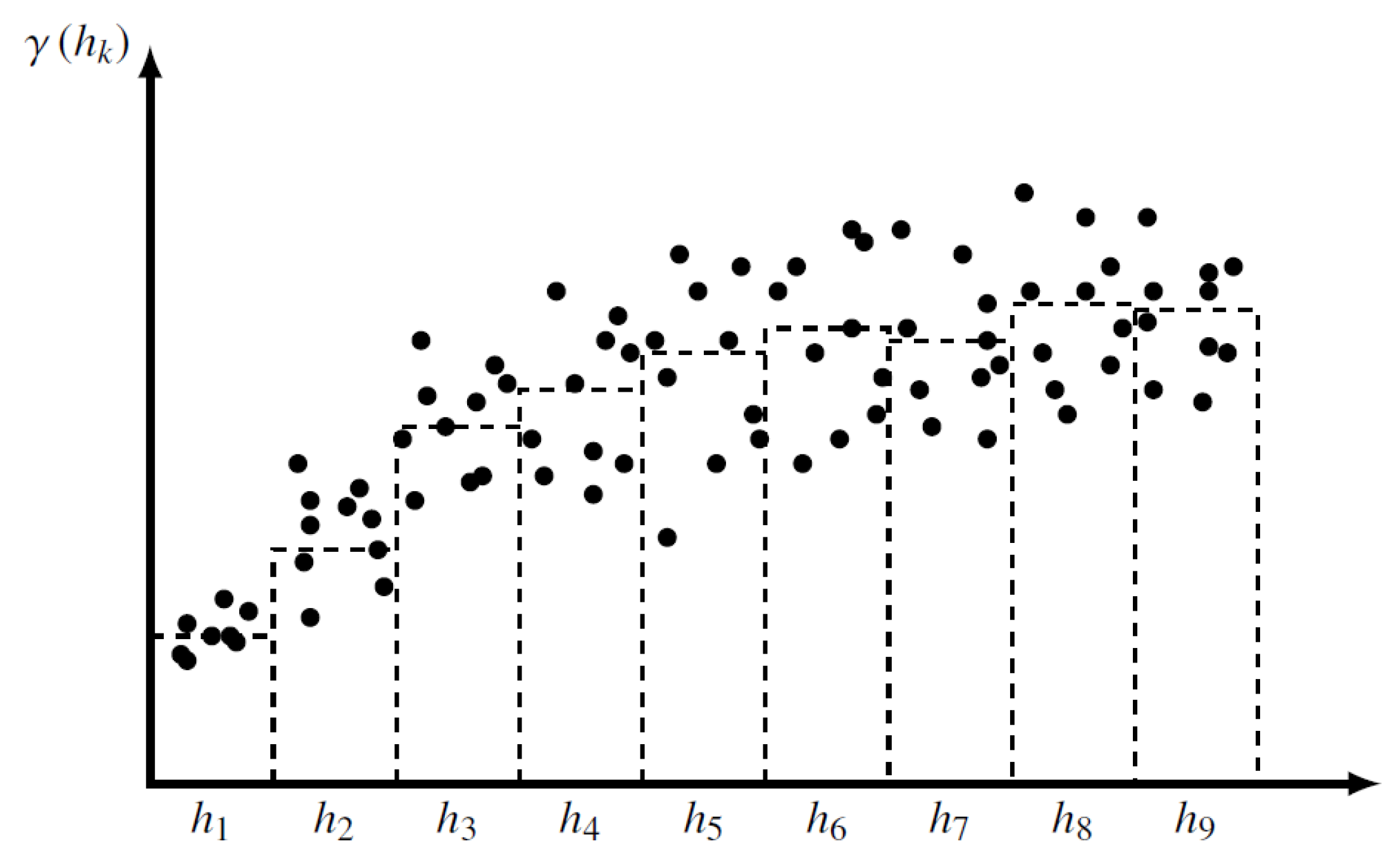
- Computing the empirical variogram function in given direction and parameters.
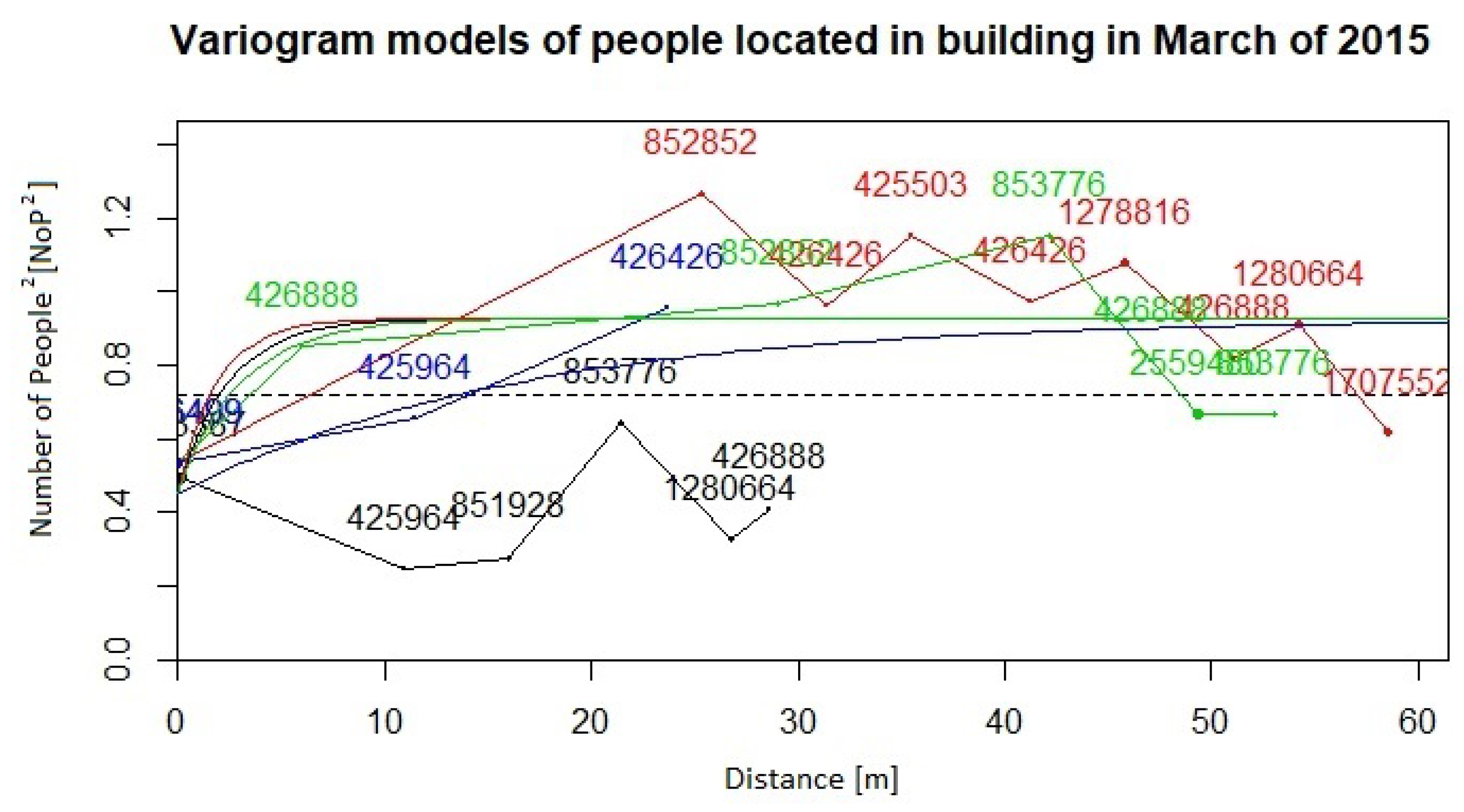
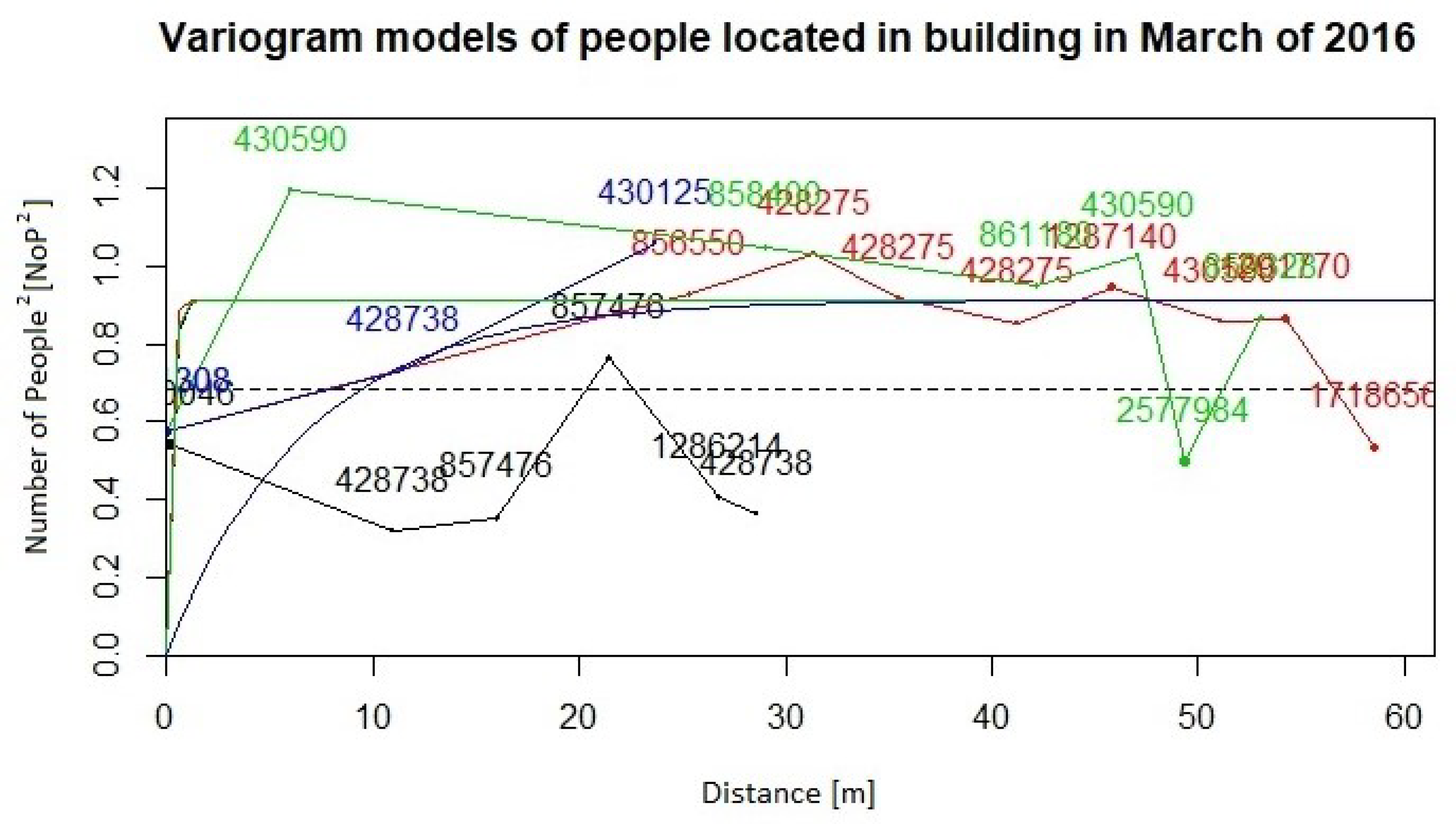
- Approximate the variogram function by fitting a parametric model for their use in the kriging conditional estimation. For both data collections from the years 2015 and 2016, we compute empirical variograms over four directions: 0, 45, 90, 135 degrees. Distance lags in each direction are 5, and the number of lags for all directions is 15. The maximum distance used for the estimation of the empirical variogram functions was 60 m for the data from both years. Afterwards, variogram functions were approximated by the exponential and spherical models. Figure 11 and Figure 12 present the empirical variograms and fitted exponential models at the four directions for the years 2015 and 2016, respectively.
- Choose appropriate parameters of TB and the number of repetitions per model.
- Run TB algorithm to compute spatial estimations of the variable of interest, , specifically in our study the values of the variable NoP at spatial location .
- Select directions in m-dimensional space so that .The covariance of the spatial process is obtained by summing the projection of the process realizations for a given number of lines of covariance .
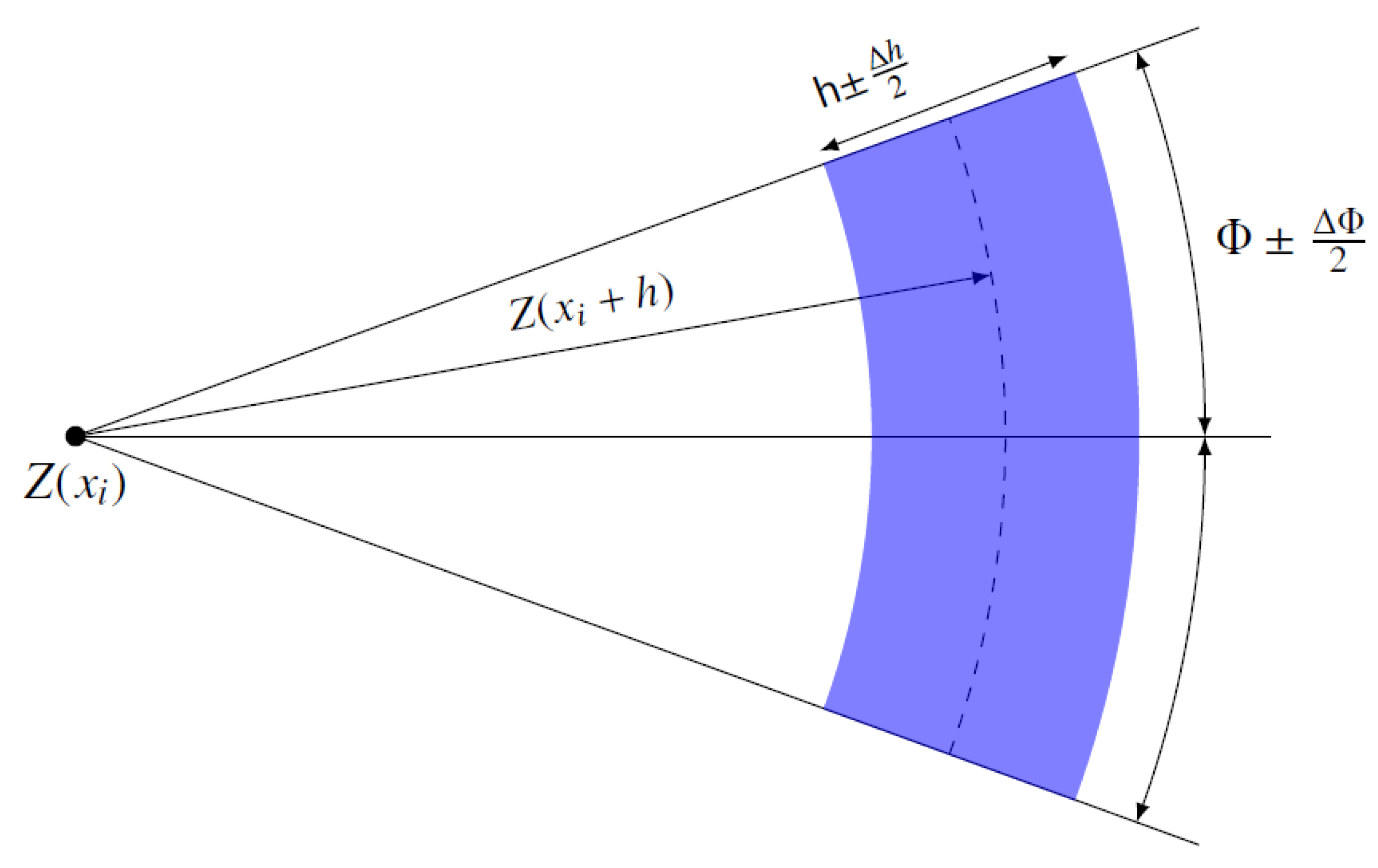
- Generate realizations of standard, independent 1D stochastic processes with covariance functions .When all the are identical to a covariance function, denoted , the relationship between and is as follows [42]:where: stands for the volume of the unit ball in m-dimensional space. In our case, , it reduces to:or equivalently:Knowing variogram and variance C(0) for a stationary random function Z is tantamount to knowing its covariance. To determine a covariance function for each variable, we compute a variogram function, which is defined for any displacement vector as:The tolerance of the directional variogram as a function of distance is illustrated in Figure 14.The directional variogram is obtained by averaging the local estimations for given line processes, as shown in Figure 15.
- Compute for each , where is the set of locations of the discretized domain where we generate the process value estimations.There is a wide variety of sampling methods for stochastic processes with a given covariance function . The most popular are the spectral, dilution, and migration methods.
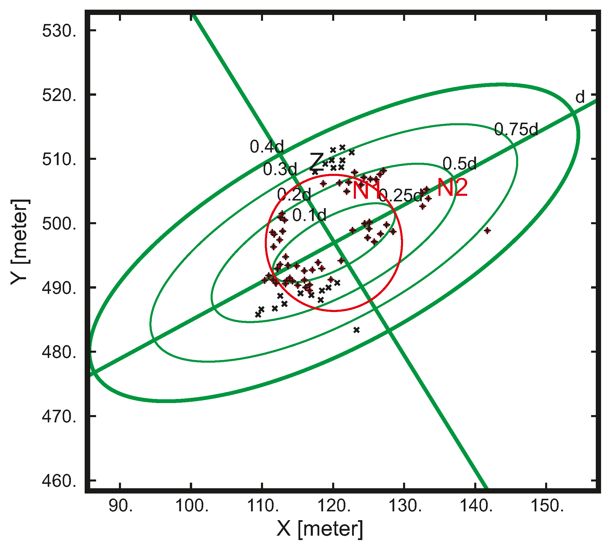
- Compute the kriged estimate for each .Let Y be a stationary Gaussian random function with average value 0, variance equal to 1, and covariance function C. The goal is to generate a sample of Y satisfying the contour conditions given be the known values at specific spatial locations . Kriging involves the resolution of a system of linear equations, requiring the definition of a set of neighborhood points. There are two types of neighborhood: unique and moving. A unique neighborhood needs only to compute once the inverse kriging matrix because it remains the same for all considered points. Thus, solutions using unique neighborhood can be computed much more quickly than moving neighborhood. When using a moving neighborhood, the closest points located in a sphere or ellipsoid are selected to be correlated with the considered point . Examples of moving neighborhood are shown in Figure 16. The moving neighborhood search in our study has been performed by angular sectors and the neighborhood ellipsoid is anisotropic in 3D.The neighborhood points are produced by an algorithm which takes into account criteria such as rotation, search ellipsoid (it defines the maximum distance along the main axes U, V, W after rotation), anisotropy, the minimum number of points considered in the range search, etc. If the neighborhood is anisotropic, the search ellipsoid is defined by:where , , and correspond with distance along the axis of the new coordinate system, and , , and correspond to the ratio between the maximum distance upon axis U, V, W and the maximum distance , respectively.
- Generate samples of a Gaussian random function with mean 0, and covariance C in domain conditioned to the contour points.Obtained values are: and .
- Calculate the kriged estimate.The Kriging estimation is given by:for each .
- Finally, we have an estimation of the values of the target random function as the result.
4. Results
5. Discussion
5.1. Effect of Crowd Size and Density
5.2. Generalization and Adaptation
5.3. Information Fusion with Other Sensor Networks
5.4. Privacy Levels
5.5. Human Interaction Analysis
5.6. Limitations
6. Conclusions
Author Contributions
Funding
Conflicts of Interest
Abbreviations
| APs | Access Points |
| NoP | Number of People |
| RSSI | Received signal strength intensity |
| TB | Turning Bands |
| WSNs | Wireless Sensor Networks |
| WUST | WrocÅaw University of Science and Technology |
References
- Breitbarth, P. The impact of GDPR one year on. Netw. Secur. 2019, 2019, 11–13. [Google Scholar] [CrossRef]
- Gioia, C.; Sermi, F.; Tarchi, D.; Vespe, M. On cleaning strategies for WiFi positioning to monitor dynamic crowds. Appl. Geomat. 2019. [Google Scholar] [CrossRef]
- Khan, M.U.K.; Park, H.; Kyung, C. Rejecting Motion Outliers for Efficient Crowd Anomaly Detection. IEEE Trans. Inf. Forensics Secur. 2019, 14, 541–556. [Google Scholar] [CrossRef]
- Huang, S.; Li, X.; Zhang, Z.; Wu, F.; Gao, S.; Ji, R.; Han, J. Body Structure Aware Deep Crowd Counting. IEEE Trans. Image Process. 2018, 27, 1049–1059. [Google Scholar] [CrossRef]
- Afiq, A.; Zakariya, M.; Saad, M.; Nurfarzana, A.; Khir, M.; Fadzil, A.; Jale, A.; Gunawan, W.; Izuddin, Z.; Faizari, M. A review on classifying abnormal behavior in crowd scene. J. Vis. Commun. Image Represent. 2019, 58, 285–303. [Google Scholar] [CrossRef]
- Shao, Y.; Mei, Y.; Chu, H.; Chang, Z.; Jing, Q.; Huang, Q.; Zhan, H.; Rao, Y. Using Multi-Scale Infrared Optical Flow-based Crowd motion estimation for Autonomous Monitoring UAV. In Proceedings of the 2018 Chinese Automation Congress (CAC), Xi’an, China, 30 November–2 December 2018; pp. 589–593. [Google Scholar] [CrossRef]
- Veganzones, M.A.; Grana, M. A Spectral/Spatial CBIR System for Hyperspectral Images. IEEE J. Sel. Top. Appl. Earth Obs. Remote Sens. 2012, 5, 488–500. [Google Scholar] [CrossRef]
- Agarwal, R.; Kumar, S.; Hegde, R.M. Algorithms for Crowd Surveillance Using Passive Acoustic Sensors over a Multimodal Sensor Network. IEEE Sens. J. 2015, 15, 1920–1930. [Google Scholar] [CrossRef]
- Yuan, Y.; Qiu, C.; Xi, W.; Zhao, J. Crowd Density Estimation Using Wireless Sensor Networks. In Proceedings of the 2011 Seventh International Conference on Mobile Ad-hoc and Sensor Networks, Beijing, China, 16–18 December 2011; pp. 138–145. [Google Scholar] [CrossRef]
- Haghani, M.; Sarvi, M. Crowd behaviour and motion: Empirical methods. Transp. Res. Part B Methodol. 2018, 107, 253–294. [Google Scholar] [CrossRef]
- Cho, S.Y.; Chow, T.W.; Leung, C.T. A neural-based crowd estimation by hybrid global learning algorithm. IEEE Trans. Syst. Man, Cybern. Part B (Cybern.) 1999, 29, 535–541. [Google Scholar] [CrossRef]
- Yan, W.; Zou, Z.; Xie, J.; Liu, T.; Li, P. The detecting of abnormal crowd activities based on motion vector. Optik 2018, 166, 248–256. [Google Scholar] [CrossRef]
- Fagette, A.; Courty, N.; Racoceanu, D.; Dufour, J.Y. Unsupervised dense crowd detection by multiscale texture analysis. Pattern Recognit. Lett. 2014, 44, 126–133. [Google Scholar] [CrossRef]
- Chong, X.; Liu, W.; Huang, P.; Badler, N.I. Hierarchical crowd analysis and anomaly detection. J. Vis. Lang. Comput. 2014, 25, 376–393. [Google Scholar] [CrossRef]
- Ge, W.; Collins, R.T. Evaluation of sampling-based pedestrian detection for crowd counting. In Proceedings of the 2009 Twelfth IEEE International Workshop on Performance Evaluation of Tracking and Surveillance, Snowbird, UT, USA, 7–9 December 2009; pp. 1–7. [Google Scholar] [CrossRef]
- Barandiaran, I.; Paloc, C.; Graña, M. Real-time optical markerless tracking for augmented reality applications. J. Real-Time Image Process. 2010, 5, 129–138. [Google Scholar] [CrossRef]
- Feng, Y.; Yuan, Y.; Lu, X. Learning deep event models for crowd anomaly detection. Neurocomputing 2017, 219, 548–556. [Google Scholar] [CrossRef]
- Ma, J.; Dai, Y.; Tan, Y.P. Atrous convolutions spatial pyramid network for crowd counting and density estimation. Neurocomputing 2019, 350, 91–101. [Google Scholar] [CrossRef]
- Zou, Z.; Cheng, Y.; Qu, X.; Ji, S.; Guo, X.; Zhou, P. Attend To Count: Crowd Counting with Adaptive Capacity Multi-scale CNNs. Neurocomputing 2019. [Google Scholar] [CrossRef]
- Cheung, E.; Wong, A.; Bera, A.; Wang, X.; Manocha, D. LCrowdV: Generating labeled videos for pedestrian detectors training and crowd behavior learning. Neurocomputing 2019, 337, 1–14. [Google Scholar] [CrossRef]
- Zhang, X.; Zhang, Q.; Hu, S.; Guo, C.; Yu, H. Energy Level-Based Abnormal Crowd Behavior Detection. Sensors 2018, 18, 423. [Google Scholar] [CrossRef]
- Mejia-Romero, S.; Lugo, J.E.; Doti, R.; Faubert, J. Assessing crowd dynamics with thermal imaging. In Proceedings of the 2016 Photonics North (PN), Quebec City, QC, Canada, 24–26 May 2016; p. 1. [Google Scholar] [CrossRef]
- Haghmohammadi, H.F.; Necsulescu, D.S.; Vahidi, M. Remote measurement of body temperature for an indoor moving crowd. In Proceedings of the 2018 IEEE International Conference on Automation, Quality and Testing, Robotics (AQTR), Cluj-Napoca, Romania, 24–26 May 2018; pp. 1–6. [Google Scholar] [CrossRef]
- Andersson, M.; Rydell, J.; Ahlberg, J. Estimation of crowd behavior using sensor networks and sensor fusion. In Proceedings of the 2009 12th International Conference on Information Fusion, Seattle, WA, USA, 6–9 July 2009; pp. 396–403. [Google Scholar]
- Pham, Q.; Gond, L.; Begard, J.; Allezard, N.; Sayd, P. Real-Time Posture Analysis in a Crowd using Thermal Imaging. In Proceedings of the 2007 IEEE Conference on Computer Vision and Pattern Recognition, Minneapolis, MN, USA, 17–22 June 2007; pp. 1–8. [Google Scholar] [CrossRef]
- Liu, G.; Wang, T.; Cao, Z. Crowd density estimation based on the normalized number of foreground pixels in infrared images. In Proceedings of the 2013 Fourth International Conference on Intelligent Control and Information Processing (ICICIP), Beijing, China, 9–11 June 2013; pp. 6–9. [Google Scholar] [CrossRef]
- Fujita, K.; Higuchi, T.; Hiromori, A.; Yamaguchi, H.; Higashino, T.; Shimojo, S. Human crowd detection for physical sensing assisted geo-social multimedia mining. In Proceedings of the 2015 IEEE Conference on Computer Communications Workshops (INFOCOM WKSHPS), Hong Kong, China, 26 April–1 May 2015; pp. 642–647. [Google Scholar] [CrossRef]
- Lykov, S.; Asakura, Y.; Hanaoka, S. Positioning in Wireless Sensor Network for Human Sensing Problem. Transp. Res. Procedia 2017, 21, 56–64. [Google Scholar] [CrossRef]
- Zou, H.; Zhou, Y.; Yang, J.; Spanos, C.J. Device-free occupancy detection and crowd counting in smart buildings with WiFi-enabled IoT. Energy Build. 2018, 174, 309–322. [Google Scholar] [CrossRef]
- Di Domenico, S.; Pecoraro, G.; Cianca, E.; De Sanctis, M. Trained-once device-free crowd counting and occupancy estimation using WiFi: A Doppler spectrum based approach. In Proceedings of the 2016 IEEE 12th International Conference on Wireless and Mobile Computing, Networking and Communications (WiMob), New York, NY, USA, 17–19 October 2016; pp. 1–8. [Google Scholar] [CrossRef]
- Lantuéjoul, C. Geostatistical Simulation: Models and Algorithms; Springer: Berlin/Heidelberg, Germany, 2002. [Google Scholar]
- Chilès, J.; Delfiner, P. Geostatistics: Modeling Spatial Uncertainty; Wiley: Hoboken, NJ, USA, 1999. [Google Scholar]
- Kamińska-Chuchmała, A.; Wilczyński, A. Spatial electric load forecasting in transmission networks with Sequential Gaussian Simulation method. Rynek Energii 2011, 1, 35–40. [Google Scholar]
- Borzemski, L.; Kamińska-Chuchmała, A. Client-perceived web performance knowledge discovery through turning bands method. Cybern. Syst. 2012, 43, 354–368. [Google Scholar] [CrossRef]
- Kamińska-Chuchmała, A. Spatial Models of Wireless Network Efficiency Prediction by Turning Bands Co-simulation Method. In Proceedings of the International Joint Conference SOCO’18-CISIS’18-ICEUTE’18, San Sebastián, Spain, 6–8 June 2018; pp. 155–164. [Google Scholar]
- Emery, X.; Lantuéjoul, C. TBSIM: A computer program for conditional simulation of three-dimensional Gaussian random fields via the turning bands method. Comput. Geosci. 2006, 32, 1615–1628. [Google Scholar] [CrossRef]
- R Core Team. R: A Language and Environment for Statistical Computing; R Foundation for Statistical Computing: Vienna, Austria, 2013. [Google Scholar]
- Renard, D.; Bez, N.; Desassis, N.; Beucher, H.; Ors, F.; Freulon, X. RGeostats: Geostatistical Package, r package version 11.2.1 ed.; 2018. Available online: https://www.r-project.org/ (accessed on 26 September 2019).
- Chentsov, N. Lévy Brownian Motion for Several Parameters and Generalized White Noise. Theory Probab. Appl. 1957, 2, 265–266. [Google Scholar] [CrossRef]
- Mantoglou, A.; Wilson, J.L. The Turning Bands Method for simulation of random fields using line generation by a spectral method. Water Resour. Res. 1982, 18, 1379–1394. [Google Scholar] [CrossRef]
- Matern, B. Spatial Variation Stochastic Models and Their Application to Some Problems in Forests Surveys and Other Sampling Investigations. Meddelanden fran Statens Skogsforskningsinstitut 1960, 49, 144. [Google Scholar]
- Matheron, G. The Intrinsic Random Functions and Their Applications. Adv. Appl. Probab. 1973, 5, 439–468. [Google Scholar] [CrossRef]
- Simon, E.; Bertino, L. Gaussian anamorphosis extension of the DEnKF for combined state parameter estimation: Application to a 1D ocean ecosystem model. J. Mar. Syst. 2012, 89, 1–18. [Google Scholar] [CrossRef]
- Wackernagel, H. Gaussian Anamorphosis with Hermite Polynomials. In Multivariate Geostatistics: An Introduction with Applications; Springer: Berlin/Heidelberg, Germany, 2003; pp. 238–249. [Google Scholar] [CrossRef]
- Feng, X.; Murray, A.T. Allocation using a heterogeneous space Voronoi diagram. J. Geogr. Syst. 2018. [Google Scholar] [CrossRef]
- Longo, S.; Cheng, B. Real-Time Privacy Preserving Crowd Estimation Based on Sensor Data. In Proceedings of the 2016 IEEE International Conference on Mobile Services (MS), San Francisco, CA, USA, 27 June–2 July 2016; pp. 95–102. [Google Scholar] [CrossRef]
- Seneviratne, S.; Hu, Y.; Nguyen, T.; Lan, G.; Khalifa, S.; Thilakarathna, K.; Hassan, M.; Seneviratne, A. A Survey of Wearable Devices and Challenges. IEEE Commun. Surv. Tutor. 2017, 19, 2573–2620. [Google Scholar] [CrossRef]
- Wang, T.; Zheng, Z.; Elhoseny, M. Equivalent mechanism: Releasing location data with errors through differential privacy. Future Gener. Comput. Syst. 2019, 98, 600–608. [Google Scholar] [CrossRef]
- Liu, B.; Cai, H.; Ju, Z.; Liu, H. RGB-D sensing based human action and interaction analysis: A survey. Pattern Recognit. 2019, 94, 1–12. [Google Scholar] [CrossRef]
- Stephens, K.; Bors, A.G. Modelling of interactions for the recognition of activities in groups of people. Digit. Signal Process. 2018, 79, 34–46. [Google Scholar] [CrossRef]
- Graña, M.; Torrealdea, F. Hierarchically structured systems. Eur. J. Oper. Res. 1986, 25, 20–26. [Google Scholar] [CrossRef]


| Period of Time | Minimum Value | Maximum Value | Mean Value | Standard Deviation | Variability Coefficient |
|---|---|---|---|---|---|
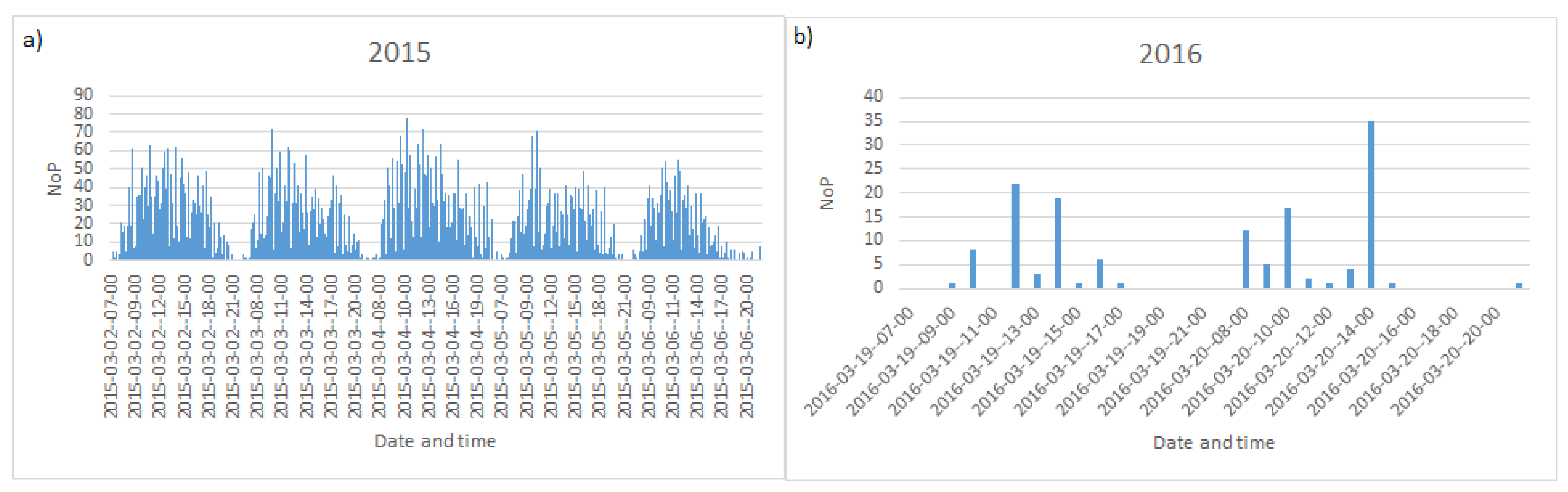
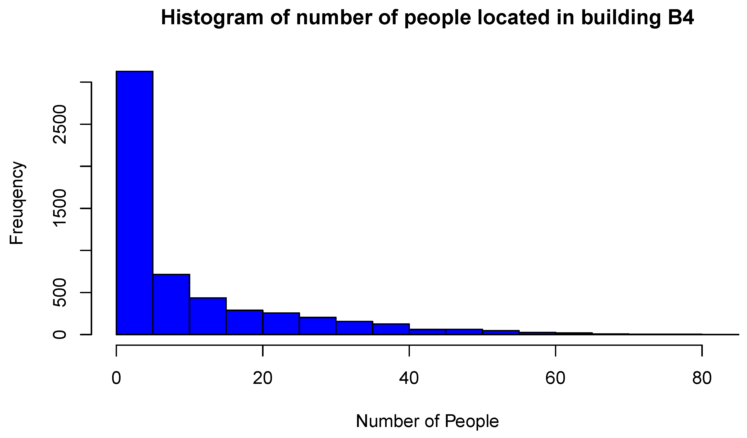
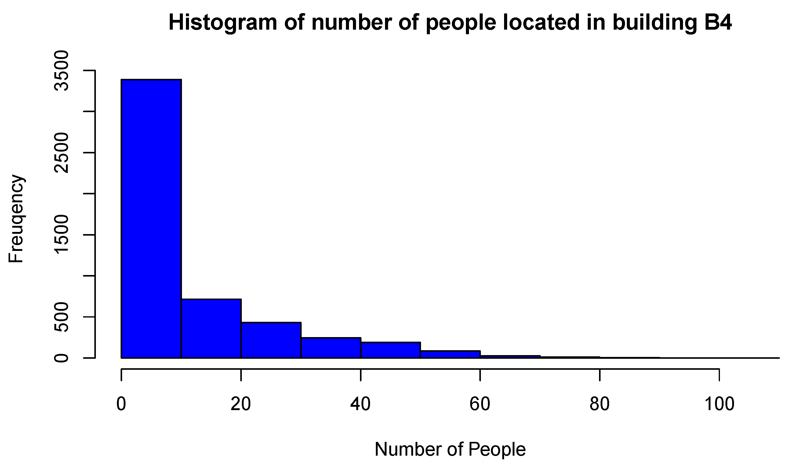
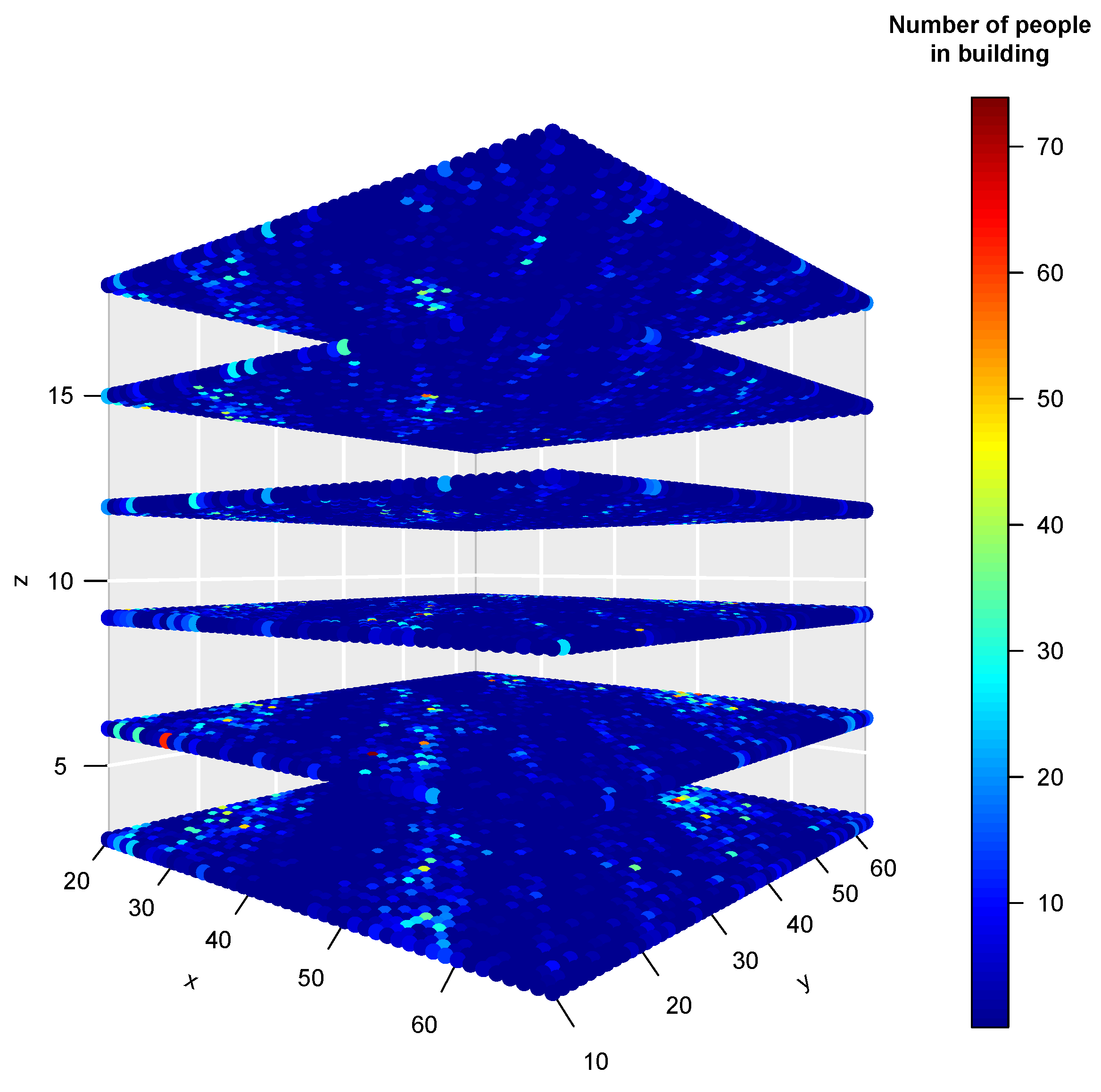
| March 2015 | 0 | 81 | 10.61 | 13.51 | 127.37 |
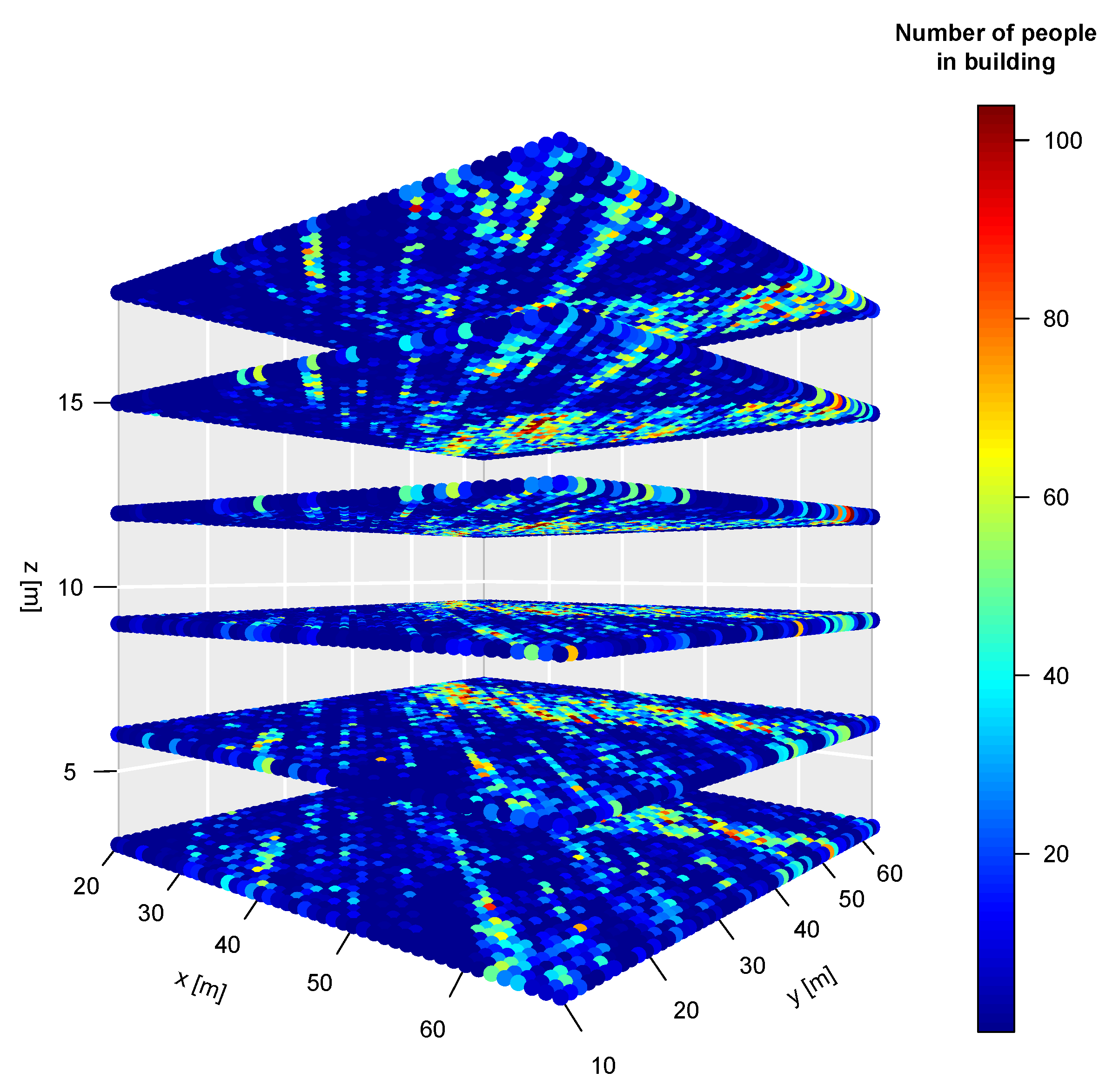
| March 2016 | 0 | 102 | 10.68 | 14.49 | 135.62 |
| Accuracy | D | L | R |
|---|---|---|---|
| mean (%) | 96 | 90 | 95 |
| std. dev. | 3.6 | 4.45 | 2.3 |
© 2019 by the authors. Licensee MDPI, Basel, Switzerland. This article is an open access article distributed under the terms and conditions of the Creative Commons Attribution (CC BY) license (http://creativecommons.org/licenses/by/4.0/).
Share and Cite
Kamińska-Chuchmała, A.; Graña, M. Indoor Crowd 3D Localization in Big Buildings from Wi-Fi Access Anonymous Data. Sensors 2019, 19, 4211. https://doi.org/10.3390/s19194211
Kamińska-Chuchmała A, Graña M. Indoor Crowd 3D Localization in Big Buildings from Wi-Fi Access Anonymous Data. Sensors. 2019; 19(19):4211. https://doi.org/10.3390/s19194211
Chicago/Turabian StyleKamińska-Chuchmała, Anna, and Manuel Graña. 2019. "Indoor Crowd 3D Localization in Big Buildings from Wi-Fi Access Anonymous Data" Sensors 19, no. 19: 4211. https://doi.org/10.3390/s19194211
APA StyleKamińska-Chuchmała, A., & Graña, M. (2019). Indoor Crowd 3D Localization in Big Buildings from Wi-Fi Access Anonymous Data. Sensors, 19(19), 4211. https://doi.org/10.3390/s19194211