A Lamb Wave Wavenumber-Searching Method for a Linear PZT Sensor Array


Abstract
1. Introduction
- (1)
- (2)
- Phase-unwrapping method [42,43]: The excitation signal and the received signal of Lamb wave are separately phase–unwrapped to obtain the phase at the center frequency of the signal. Then, according to the wavenumber definition formula, the wavenumber of the Lamb wave can be calculated using the propagation distance. However, for unknown excitation signal or propagation distance of the Lamb wave, or for complex signal components, this method is difficult to use.
- (3)
- Fourier-transform method [44,45,46]: According to the definition of the wavenumber, the wavenumber of Lamb wave can be obtained by the Fourier transform of the Lamb wave spatial sampling signal. This method generally requires a higher spatial sampling rate and longer spatial sampling length according to the properties of the Fourier transform. Therefore, this method is generally used to process Lamb wave spatial signals collected by scanning laser Doppler vibrometer (SLDV). However, it is inappropriate for use in online damage monitoring.
- (4)
- Spatial-wavenumber filter method [34,35,36,37,47]: A series of spatial-wavenumber filters with different central wavenumbers are used to filter the spatial sampling signal of the Lamb wave. When the scanning wavenumber is equal to the wavenumber of the Lamb wave spatial sampling signal, the Lamb wave spatial sampling signal is able to pass the spatial–wavenumber filter. The wavenumber of the Lamb wave spatial sampling signal is then obtained. The spatial sampling rate of the linear PZT sensor array should satisfy the Nyquist sampling theorem in this method.
2. The Lamb Wave Wavenumber-Searching Method
2.1. Theoretic Foundations of the Method
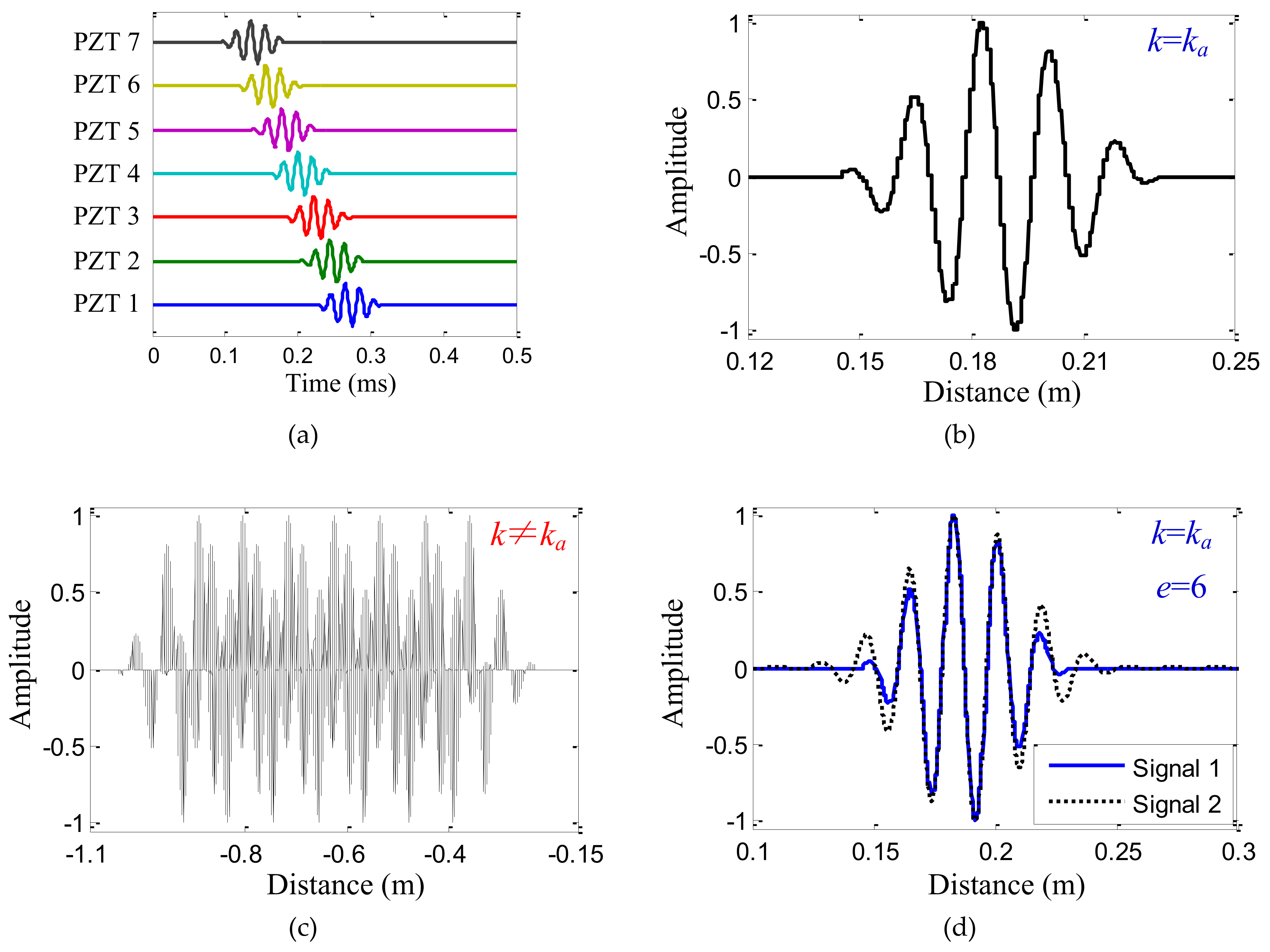
2.2. The Principle of the Method
3. Damage Localization Based on the Lamb Wave Wavenumber–Searching Method and Cruciform PZT Sensor Array
4. Validation Experiment of the Lamb Wave Wavenumber-Searching Method
4.1. Experimental Setup
4.2. Theoretical Wavenumber Calculation
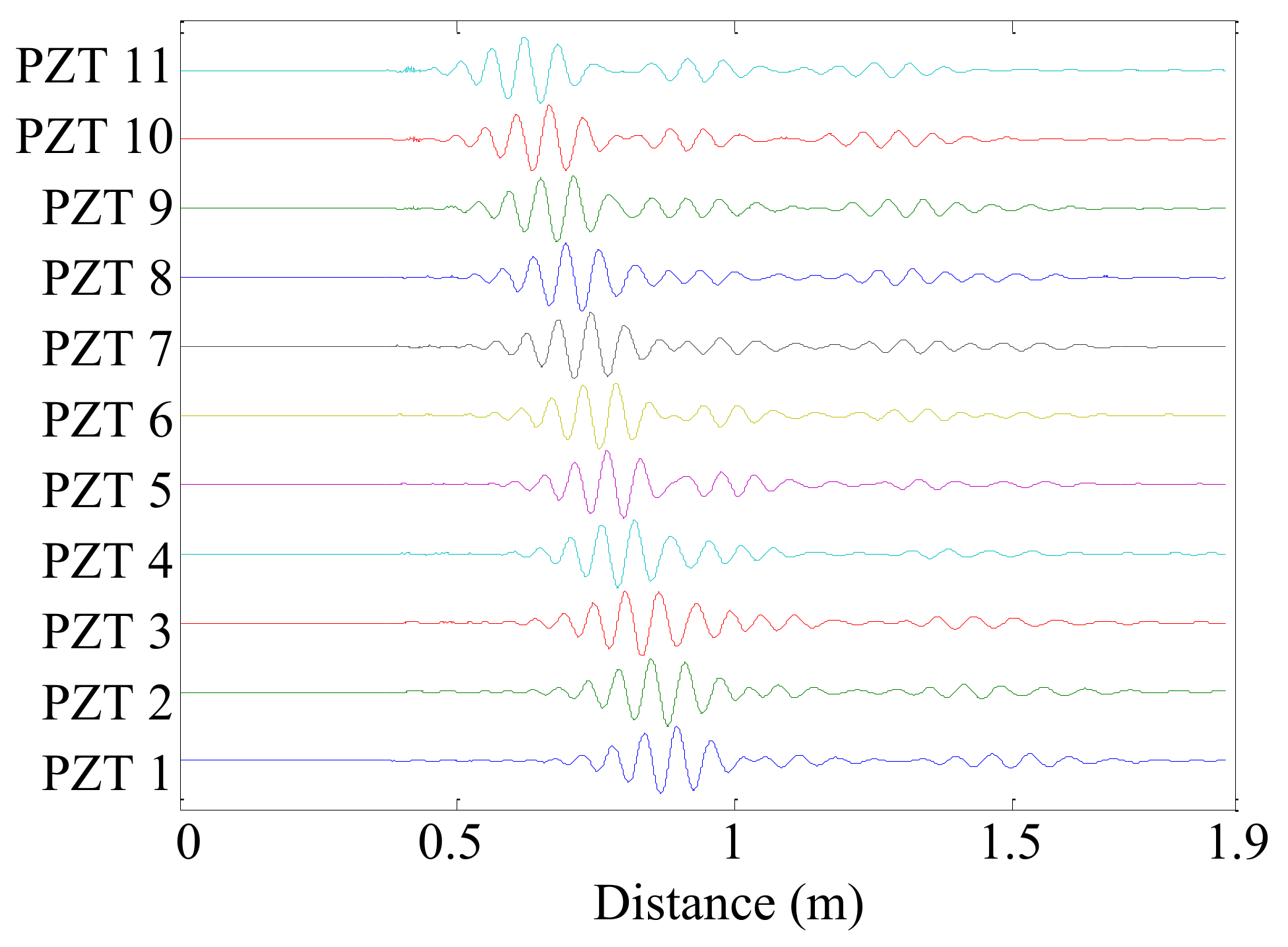
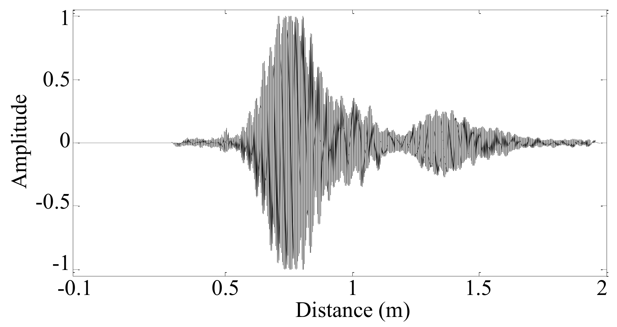
4.3. Typical Signal Analysis
5. Validation of the Damage Localization Method
5.1. Experimental Setup
- (1)
- The group velocity of Lamb wave was measured using the continuous complex Shannon wavelet transformation. The actuator was used to excite Lamb wave propagating on the composite plate, while the three reference PZT sensors were used to acquire the corresponding Lamb wave. For each reference PZT sensor, the group velocity was calculated as cg-Ref 1 = 1569.32 m/s, cg-Ref 2 = 1557.29 m/s, and cg-Ref 3 = 1485.65 m/s. Then, the average group velocity cg = 1537.42 m/s was obtained and used in damage localization.
- (2)
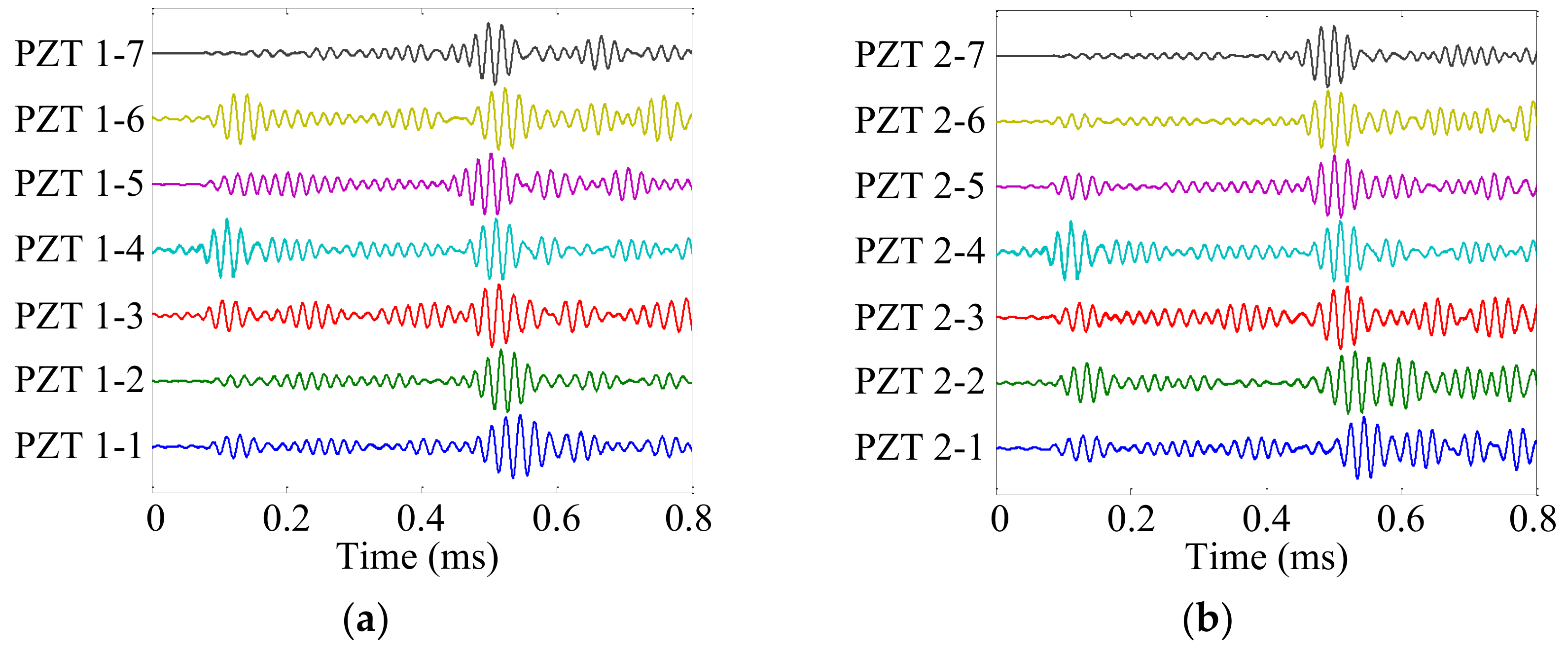
- In the health state of the carbon fiber composite laminate plate, the Lamb wave signals of the cruciform PZT sensor array were acquired as health reference signals, fHR.
- (3)
- Damage is created in each position and the corresponding Lamb wave signals of the cruciform PZT sensor array were acquired as the online monitoring signals, fOM.
5.2. Damage Localization Validation
6. Conclusions
Author Contributions
Funding
Acknowledgments
Conflicts of Interest
References
- Boller, C. Next generation structural health monitoring and its integration into aircraft design. Int. J. Syst. Sci. 2000, 31, 1333–1349. [Google Scholar] [CrossRef]
- Ihn, J.B.; Chang, F.K. Pitch-catch active sensing methods in structural health monitoring for aircraft structures. Struct. Health Monit. 2008, 7, 5–19. [Google Scholar] [CrossRef]
- Mitra, M.; Gopalakrishnan, S. Guided wave based structural health monitoring: A review. Smart Mater. Struct. 2016, 25, 053001. [Google Scholar] [CrossRef]
- Su, Z.; Ye, L.; Lu, Y. Guided Lamb waves for identification of damage in composite structures: A review. J. Sound Vib. 2006, 295, 753–780. [Google Scholar] [CrossRef]
- Migot, A.; Bhuiyan, Y.; Giurgiutiu, V. Numerical and experimental investigation of damage severity estimation using Lamb wave-based imaging methods. J. Intell. Mater. Syst. Struct. 2019, 30, 618–635. [Google Scholar] [CrossRef]
- Qing, X.; Li, W.; Wang, Y.; Sun, H. Piezoelectric transducer-based structural health monitoring for aircraft applications. Sensors 2019, 19, 545. [Google Scholar] [CrossRef]
- Rao, J.; Ratassepp, M.; Lisevych, D.; Hamzah Caffoor, M.; Fan, Z. On-line corrosion monitoring of plate structures based on guided wave tomography using piezoelectric sensors. Sensors 2017, 17, 2882. [Google Scholar] [CrossRef]
- Zhou, W.; Li, H.; Yuan, F.G. Fundamental understanding of wave generation and reception using d36 type piezoelectric transducers. Ultrasonics 2015, 57, 135–143. [Google Scholar] [CrossRef]
- Qiu, L.; Liu, M.; Qing, X.; Yuan, S. A quantitative multidamage monitoring method for large-scale complex composite. Struct. Health Monit. 2013, 12, 183–196. [Google Scholar] [CrossRef]
- Fu, S.; Shi, L.; Zhou, Y.; Fu, Z. Enhancement of Lamb wave imaging resolution by step pulse excitation and prewarping. Shock Vib. 2015, 1, 1–8. [Google Scholar] [CrossRef]
- Lu, G.; Li, Y.; Wang, T.; Xiao, H.; Huo, L.; Song, G. A multi-delay-and-sum imaging algorithm for damage detection using piezoceramic transducers. J. Intell. Mater. Syst. Struct. 2016, 28, 1–10. [Google Scholar] [CrossRef]
- Cai, J.; Shi, L.; Yuan, S.; Shao, Z. High spatial resolution imaging for structural health monitoring based on virtual time reversal. Smart Mater. Struct. 2011, 20, 055018. [Google Scholar] [CrossRef]
- Zhu, R.; Huang, G.L.; Yuan, F.G. Fast damage imaging using the time-reversal technique in the frequency-wavenumber domain. Smart Mater. Struct. 2013, 22, 075028. [Google Scholar] [CrossRef]
- Mori, N.; Biwa, S.; Kusaka, T. Damage localization method for plates based on the time reversal of the mode-converted lamb waves. Ultrasonics 2018, 91, 19. [Google Scholar] [CrossRef] [PubMed]
- Wu, Z.; Liu, K.; Wang, Y.; Zheng, Y. Validation and evaluation of damage identification using probability-based diagnostic imaging on a stiffened composite panel. J. Intell. Mater. Syst. Struct. 2015, 26, 2181–2195. [Google Scholar] [CrossRef]
- Zhou, C.; Wang, Q.; Su, Z.; Cheng, L.; Hong, M. Evaluation of fatigue cracks using nonlinearities of acousto-ultrasonic waves acquired by an active sensor network. Smart Mater. Struct. 2013, 22, 015018. [Google Scholar] [CrossRef]
- Liu, Z.; Zhong, X.; Dong, T.; He, C.; Wu, B. Delamination detection in composite plates by synthesizing time-reversed Lamb waves and a modified damage imaging algorithm based on RAPID. Struct. Control Health 2017, 24, e1919. [Google Scholar] [CrossRef]
- Tofeldt, O.; Ryden, N. Lamb wave phase velocity imaging of concrete plates with 2D arrays. J. Nondestruct. Eval. 2018, 37, 4. [Google Scholar] [CrossRef]
- Liu, Z.; Sun, K.; Song, G.; He, C.; Wu, B. Damage localization in aluminum plate with compact rectangular phased piezoelectric transducer array. Mech. Syst. Signal Process. 2016, 70, 625–636. [Google Scholar] [CrossRef]
- Yu, L.; Tian, Z. Guided wave phased array beamforming and imaging in composite plates. Ultrasonics 2016, 68, 43–53. [Google Scholar] [CrossRef]
- Bao, Q.; Yuan, S.; Guo, F.; Qiu, L. Transmitter beamforming and weighted image fusion–based multiple signal classification algorithm for corrosion monitoring. Struct. Health Monit. 2019, 18, 621–634. [Google Scholar] [CrossRef]
- Zhong, Y.; Xiang, J.; Chen, X.; Jiang, Y.; Pang, J. Multiple signal classification-based impact localization in composite structures using optimized ensemble empirical mode decomposition. Appl. Sci. Basel 2018, 8, 1447. [Google Scholar] [CrossRef]
- Zuo, H.; Yang, Z.; Xu, C.; Tian, S.; Chen, X. Damage identification for plate-like structures using ultrasonic guided wave based on improved MUSIC method. Compos. Struct. 2018, 203, 164–171. [Google Scholar] [CrossRef]
- Bao, Q.; Yuan, S.; Wang, Y.; Qiu, L. Anisotropy compensated MUSIC algorithm based composite structure damage imaging method. Compos. Struct. 2019, 214, 293–303. [Google Scholar] [CrossRef]
- Chen, X.; Xu, K. Propagation characteristic of ultrasonic lamb wave. Appl. Mech. Mater. 2012, 157–158, 987–990. [Google Scholar] [CrossRef]
- Peddeti, K.; Santhanam, S. Dispersion curves for Lamb wave propagation in prestressed plates using a semi-analytical finite element analysis. J. Acoust. Soc. Am. 2018, 143, 829–840. [Google Scholar] [CrossRef]
- Yanyu, M.; Shi, Y. Thin plate lamb propagation rule and dispersion curve drawing based on wave theory. Surf. Rev. Lett. 2018, 26, 1850222. [Google Scholar] [CrossRef]
- Kannajosyula, H.; Lissenden, C.J.; Rose, J.L. Analysis of annular phased array transducers for ultrasonic guided wave mode control. Smart Mater. Struct. 2013, 22, 085019. [Google Scholar] [CrossRef]
- Mckeon, P.; Yaacoubi, S.; Declercq, N.F.; Ramadan, S.; Yaacoubi, W.K. Baseline subtraction technique in the frequency–wavenumber domain for high sensitivity damage detection. Ultrasonics 2014, 54, 592–603. [Google Scholar] [CrossRef] [PubMed]
- Cai, J.; Yuan, S.; Qing, X.P.; Chang, F.K.; Shi, L.; Qiu, L. Linearly dispersive signal construction of Lamb waves with measured relative wavenumber curves. Sens. Actuators A Phys. 2015, 221, 41–52. [Google Scholar] [CrossRef]
- Rogge, M.D.; Leckey, C.A. Characterization of impact damage in composite laminates using guided wavefield imaging and local wavenumber domain analysis. Ultrasonics 2013, 53, 1217–1226. [Google Scholar] [CrossRef] [PubMed]
- Tian, Z.; Yu, L. Lamb wave frequency-wavenumber analysis and decomposition. J. Intell. Mater. Syst. Struct. 2014, 25, 1107–1123. [Google Scholar] [CrossRef]
- Purekar, A.S.; Pines, D.J. Damage detection in thin composite laminates using piezoelectric phased sensor arrays and guided lamb wave interrogation. J. Intell. Mater. Syst. Struct. 2010, 21, 995–1010. [Google Scholar] [CrossRef]
- Qiu, L.; Liu, B.; Yuan, S. Impact imaging of aircraft composite structure based on a model-independent spatial-wavenumber filter. Ultrasonics 2016, 64, 10–24. [Google Scholar] [CrossRef] [PubMed]
- Qiu, L.; Liu, B.; Yuan, S.; Su, Z.; Ren, Y. A scanning spatial-wavenumber filter and PZT 2-D cruciform array based on-line damage imaging method of composite structure. Sens. Actuators A Phys. 2016, 248, 62–72. [Google Scholar] [CrossRef]
- Ren, Y.; Qiu, L.; Yuan, S.; Bao, Q. On-Line Multi-Damage Scanning Spatial-Wavenumber Filter Based Imaging Method for Aircraft Composite Structure. Materials 2017, 10, 519. [Google Scholar] [CrossRef]
- Ren, Y.; Qiu, L.; Yuan, S.; Su, Z. A diagnostic imaging approach for online characterization of multi-impact in aircraft composite structures based on a scanning spatial-wavenumber filter of guided wave. Mech. Syst. Signal Process. 2017, 90, 44–63. [Google Scholar] [CrossRef]
- Ostachowicz, W.; Kudela, P.; Krawczuk, M.; Zak, A. Guided Waves in Structures for SHM: The Time-Domain Spectral Element Method; John Wiley & Sons: London, UK, 2011. [Google Scholar]
- Rucka, M. Modelling of in-plane wave propagation in a plate using spectral element method and Kane–Mindlin theory with application to damage detection. Arch. Appl. Mech. 2011, 81, 1877–1888. [Google Scholar] [CrossRef]
- Żak, A. A novel formulation of a spectral plate element for wave propagation in isotropic structures. Finite Elem. Anal. Des. 2009, 45, 650–658. [Google Scholar] [CrossRef]
- Palacz, M. Spectral Methods for Modelling of Wave Propagation in Structures in Terms of Damage Detection—A Review. Appl. Sci. Basel 2018, 8, 1124. [Google Scholar] [CrossRef]
- Mesnil, O.; Leckey, C.A.C.; Ruzzene, M. Instantaneous and local wavenumber estimations for damage quantification in composites. Struct. Health Monit. 2015, 14, 193–204. [Google Scholar] [CrossRef]
- Mesnil, O.; Yan, H.; Ruzzene, M.; Paynabar, K.; Shi, J. Fast wavenumber measurement for accurate and automatic location and quantification of defect in composite. Struct. Health Monit. 2016, 15, 223–234. [Google Scholar] [CrossRef]
- Yu, L.; Leckey, C.A.C.; Tian, Z. Study on crack scattering in aluminum plates with Lamb wave frequency-wavenumber analysis. Smart Mater. Struct. 2013, 22, 065019. [Google Scholar] [CrossRef]
- Fu, S.; Shi, L.; Zhou, Y.; Cai, J. Dispersion compensation in lamb wave defect detection with step-pulse excitation and warped frequency transform. IEEE Trans. Ultrason. Ferroelectr. Freq. Control 2014, 61, 2075–2088. [Google Scholar] [CrossRef] [PubMed]
- Cai, J.; Shi, L.; Qing, X.P. A time–distance domain transform method for Lamb wave dispersion compensation considering signal waveform correction. Smart Mater. Struct. 2013, 22, 105024. [Google Scholar] [CrossRef]
- Yu, L.; Tian, Z.; Leckey, C.A.C. Crack imaging and quantification in aluminum plates with guided wave wavenumber analysis methods. Ultrasonics 2015, 62, 203–212. [Google Scholar] [CrossRef] [PubMed]
- Liu, B.; Liu, T.; Meng, F. Research on Morlet wavelet based lamb wave spatial sampling signal optimization method. J. Shanghai Jiaotong Univ. Sci. 2018, 23, 62–69. [Google Scholar] [CrossRef]
- Qiu, L.; Yuan, S.F. On development of a multi-channel PZT array scanning system and its evaluating application on UAV wing box. Sens. Actuators A Phys. 2009, 151, 220–230. [Google Scholar] [CrossRef]
- Zhang, G.; Gao, W.; Song, G.; Song, Y. An imaging algorithm for damage detection with dispersion compensation using piezoceramic induced lamb waves. Smart Mater. Struct. 2017, 26, 025017. [Google Scholar] [CrossRef]


| Parameter | Value |
|---|---|
| Density / (kg·m-3) | 2.78×10³ |
| Elastic modulus / GPa | 73.1 |
| Shear modulus / GPa | 28 |
| Poisson ratio µ | 0.33 |
| Frequency (kHz) | Theoretical Wavenumber (rad/m) |
|---|---|
| 30 | 261.67 |
| 35 | 283.63 |
| 40 | 304.26 |
| 45 | 323.83 |
| 50 | 342.53 |
| 55 | 360.47 |
| 60 | 377.78 |
| 65 | 394.54 |
| 70 | 410.82 |
| Signal Source | Frequency (kHz) | Theoretical Wavenumber (rad/m) | Lamb Wave Wavenumber-Searching Method (rad/m) | Wavenumber Error (rad/m) |
|---|---|---|---|---|
| PZT A | 30 | 261.67 | 259.8 | −1.9 |
| 35 | 283.63 | 282.3 | −1.3 | |
| 40 | 304.26 | 302.5 | −1.8 | |
| 45 | 323.83 | 325.3 | 1.5 | |
| 50 | 342.53 | 340.4 | −2.1 | |
| 55 | 360.47 | 358.8 | −1.7 | |
| 60 | 377.78 | 375.6 | −2.2 | |
| 65 | 394.54 | 393.1 | −1.4 | |
| 70 | 410.82 | 408.8 | −2.0 | |
| PZT B | 30 | 130.84 | 131.5 | 0.7 |
| 35 | 141.82 | 142.6 | 0.8 | |
| 40 | 152.13 | 153.6 | 1.5 | |
| 45 | 161.92 | 161.7 | −0.2 | |
| 50 | 171.27 | 171.2 | −0.1 | |
| 55 | 180.24 | 179.9 | −0.3 | |
| 60 | 188.89 | 188.2 | −0.7 | |
| 65 | 197.27 | 196.8 | −0.5 | |
| 70 | 205.41 | 204.9 | −0.5 | |
| PZT C | 30 | −168.20 | −166.3 | 1.9 |
| 35 | −182.31 | −180.6 | 1.7 | |
| 40 | −195.57 | −193.7 | 1.9 | |
| 45 | −208.15 | −206.9 | 1.3 | |
| 50 | −220.17 | −218.2 | 2.0 | |
| 55 | −231.71 | −231.0 | 0.7 | |
| 60 | −242.83 | −242.0 | 0.8 | |
| 65 | −253.61 | −252.5 | 1.1 | |
| 70 | −264.07 | −262.1 | 2.0 |
| Parameter | Value |
|---|---|
| 0° tensile modulus (GPa) | 135 |
| 90° tensile modulus (GPa) | 8.8 |
| ± 45° in-plane shearing modulus (GPa) | 4.47 |
| Poisson ratio µ | 0.328 |
| Density (kg·m-3) | 1.61 × 10³ |
| Position Label | Cartesian Coordinates (mm, mm) | Polar Coordinates (°, mm) |
|---|---|---|
| Ref 1 | (200, 0) | (0.0, 200.0) |
| Ref 2 | (200, 200) | (45.0, 282.8) |
| Ref 3 | (0, 400) | (90.0, 400.0) |
| A | (100, 300) | (71.6, 316.2) |
| B | (100, 200) | (63.4, 223.6) |
| C | (0, 200) | (90.0, 200.0) |
| D | (−100, 200) | (116.6, 223.6) |
| E | (−200, 200) | (135.0, 282.8) |
| F | (−200, 100) | (153.4, 223.6) |
| G | (−200, 0) | (180.0, 200.0) |
| Damage Label | kn1 (rad/m) | kn2 (rad/m) | Arrive Time (ms) | Start Time (ms) | Localized Position (mm, mm) | Actual Position (mm, mm) | Damage Localization Error (mm) |
|---|---|---|---|---|---|---|---|
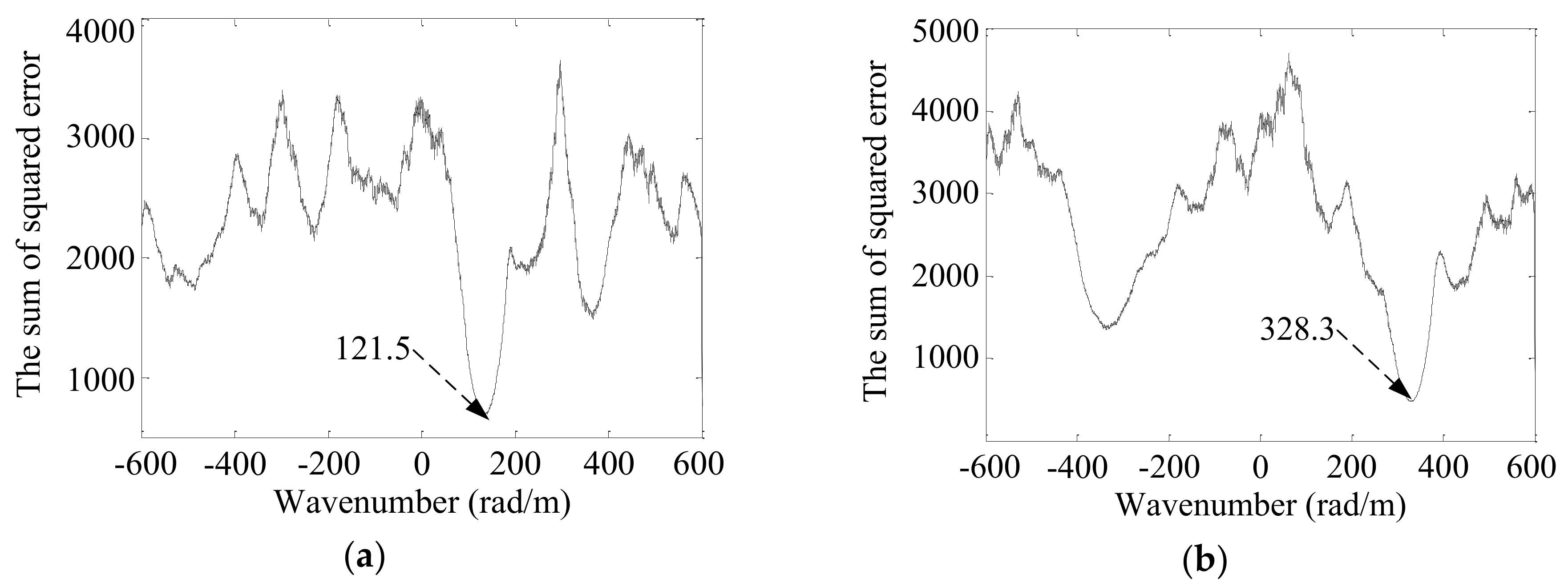
| A | 121.5 | 328.3 | 0.5124 | 0.1032 | (109.2, 295.0) | (100, 300) | 10.4 |
| B | 163.1 | 299.8 | 0.4094 | 0.1034 | (112.4, 206.6) | (100, 200) | 14.1 |
| C | 4.8 | 340.3 | 0.3583 | 0.1034 | (2.8, 195.9) | (0, 200) | 4.9 |
| D | −152.4 | 304.7 | 0.3861 | 0.1034 | (−97.2, 194.4) | (−100, 200) | 6.3 |
| E | −241.7 | 228.9 | 0.4570 | 0.1034 | (−197.4, 186.9) | (−200, 200) | 13.4 |
| F | −309.2 | 151.5 | 0.4001 | 0.1031 | (−205.0, 100.5) | (−200, 100) | 5.0 |
| G | −343.1 | −9.3 | 0.3897 | 0.1031 | (−220.0, −6.0) | (−200, 0) | 21.1 |
© 2019 by the authors. Licensee MDPI, Basel, Switzerland. This article is an open access article distributed under the terms and conditions of the Creative Commons Attribution (CC BY) license (http://creativecommons.org/licenses/by/4.0/).
Share and Cite
Liu, B.; Liu, T.; Zhao, J. A Lamb Wave Wavenumber-Searching Method for a Linear PZT Sensor Array. Sensors 2019, 19, 4166. https://doi.org/10.3390/s19194166
Liu B, Liu T, Zhao J. A Lamb Wave Wavenumber-Searching Method for a Linear PZT Sensor Array. Sensors. 2019; 19(19):4166. https://doi.org/10.3390/s19194166
Chicago/Turabian StyleLiu, Bin, Tingzhang Liu, and Jianfei Zhao. 2019. "A Lamb Wave Wavenumber-Searching Method for a Linear PZT Sensor Array" Sensors 19, no. 19: 4166. https://doi.org/10.3390/s19194166
APA StyleLiu, B., Liu, T., & Zhao, J. (2019). A Lamb Wave Wavenumber-Searching Method for a Linear PZT Sensor Array. Sensors, 19(19), 4166. https://doi.org/10.3390/s19194166