Article

Radial Basis Functions Intended to Determine the Upper Bound of Absolute Dynamic Error at the Output of Voltage-Mode Accelerometers

by
Krzysztof Tomczyk
1,*,
Marcin Piekarczyk
2 and
Grzegorz Sokal
2
1
Faculty of Electrical and Computer Engineering, Cracow University of Technology, Warszawska 24, 31-155 Krakow, Poland
2
Faculty of Mathematics, Physics and Technical Science, Pedagogical University of Cracow, 2 Podchorazych Ave, 30-084 Krakow, Poland
*
Author to whom correspondence should be addressed.
Sensors 2019, 19(19), 4154; https://doi.org/10.3390/s19194154
Submission received: 3 September 2019 / Revised: 19 September 2019 / Accepted: 23 September 2019 / Published: 25 September 2019
(This article belongs to the Section Physical Sensors)

Abstract

:
In this paper, we propose using the radial basis functions (RBF) to determine the upper bound of absolute dynamic error (UAE) at the output of a voltage-mode accelerometer. Such functions can be obtained as a result of approximating the error values determined for the assumed-in-advance parameter variability associated with the mathematical model of an accelerometer. This approximation was carried out using the radial basis function neural network (RBF-NN) procedure for a given number of the radial neurons. The Monte Carlo (MC) method was also applied to determine the related error when considering the uncertainties associated with the parameters of an accelerometer mathematical model. The upper bound of absolute dynamic error can be a quality ratio for comparing the errors produced by different types of voltage-mode accelerometers that have the same operational frequency bandwidth. Determination of the RBFs was performed by applying the Python-related scientific packages, while the calculations related both to the UAE and the MC method were carried out using the MathCad program. Application of the RBFs represent a new approach for determining the UAE. These functions allow for the easy and quick determination of the value of such errors.

1. Introduction

Acceleration, which is measured by accelerometers [1,2,3], is a feature of which instantaneous values are constantly changing [4]. A similar situation occurs when measuring other dynamic quantities (e.g., pressure, temperature, etc.) [5,6,7,8]. For those quantities, no explicit comparative criterion [9] has been developed so far, as is the case with the accuracy class of the instruments intended for static measurements [10,11]. When measuring acceleration, as is the case with other dynamic quantities [12,13,14,15], it is convenient to use the two best-known quality factors: The integral-square error [9,16,17] and the absolute error [12]. The first factor, for the assumed time of testing, allows one to determine the value of signal energy at the output of the sensor, while the second factor measures the maximum value of magnitude of this signal. However, both of these factors allow the determination of the numerical values of dynamic error for any measurement signal [9,12,13,14,15,17,18,19]. After the time corresponding to the time of the steady state of the sensor impulse response, the time characteristic of the integral-square error is linear [16,19], while the absolute error takes a constant value in time [12,18]. The time that it takes for the steady state of impulse response can be considered to be transient due to its very short duration.
Since the set of dynamic signals at the sensor input is infinite [9], in order to determine the upper bound of dynamic error [9,12,13,14] for the considered quality factor, the critical case of the input signal with limitations [20] should be determined. It can be carried out using the dedicated calculation algorithm intended for this purpose [12,13,14,15,18,19]. For the needs of such an algorithm, it is necessary to know the parameters of the mathematical model [2,3,4] of the considered sensor. Taking into account that from a practical point of view, only the error for the sensor’s operating band is of interest for the purposes of implementing such an algorithm, it is necessary to use the special standard as a reference to determine the error [9,12,21].
The main subject of this paper is the absolute dynamic error (UAE) for the absolute error criterion [12]. It is produced by the signal with limitations on both the magnitude and its duration [16,20]. An example of testing a voltage-mode accelerometer was considered in this work. It was assumed that the accelerometer is a low-pass system with an operating band limited by the cut-off frequency. Examples of the numerical values of the UAE for any time of accelerometer testing are presented in [17,18,19]. In addition, polynomial approximation was performed in [18] to determine the relationship between the error and the time of sensor testing. It was carried out using the Curve Fitting toolbox [22] built into MATLAB software. However, this type of approximation has a significant limitation due to the difficulties of determining the optimal order of the polynomial approximating the error [23,24]. Therefore, based on the Neural Network toolbox [25] built into MATLAB, the procedure for determining the optimal order of the polynomial approximating the error was presented in [26,27]. However, neither the structure nor the parameters of this polynomial were determined there.
This paper proposes the use of the radial basis function neural network (RBF-NN) to determine the RBFs [28,29,30,31,32] for an assumed number of radial neurons. In this work, the RBFs were obtained using Python-related scientific packages that allow the easy and quick determination of the upper bound of absolute dynamic error. The error obtained based on the RBF is denoted below as the U A E R B F . The RBFs were determined on the basis of previously obtained values of the UAE for the assumed-in-advance ranges of variability of the accelerometer model parameters. Section 3 presents the mathematical models with associated descriptions of both the voltage-mode accelerometer and the model of the standard, which is the reference for determining the error. Based on these models, Section 4 presents a detailed description, along with the relevant mathematical relations of the algorithm used for determining the UAE. Then, Section 5 discusses the procedure used for determining the RBF.
The values of the accelerometer model parameters intended for substitution into the RBF can be assumed in advance or obtained as a result of the parametric identification of such a model. In order to precisely determine both the parameters of the model and the associated uncertainties, the identification procedure should be based on the measurement points of both frequency responses (amplitude and phase). For this purpose, it is convenient to use the weighted-least-squares (WLS) method discussed in detail in [33,34].
When the parameters and uncertainties are assumed-in-advance or obtained on the basis of the WLS method, it is not possible to apply the RBF directly because it is unclear for which values of the parameters from the ranges determined by the associated uncertainties the maximum error can be obtained. This maximum error is denoted below as the UAERBF(max). It is therefore necessary to use a parametric optimization method to determine this error. The solution of using the Monte Carlo (MC) method [34,35,36] based on a pseudorandom number generator with uniform distribution is discussed in detail in Section 6. It was convenient to employ here the Wichmann–Hill generator [37], which is recommended by the guide [34].
Section 7 presents the matrix containing the values of the UAE. These errors were determined for the case of changes of two parameters of a voltage-mode accelerometer for the assumed-in-advance ranges of these changes and quantization steps. Based on the matrix of errors, the optimal order, structure, and parameters values of the RBF were determined. The 5, 10, and 15 radial neurons were considered. Based on these functions, the error UAERBF was determined for the selected values of the accelerometer parameters. Then, the values of uncertainties were assumed for the parameters and the UAERBF(max) values were calculated by employing the MC method.
The procedure for determining the RBF function as well as an application of the MC method to establish the error UAERBF constitute the novelty of this paper.

2. General Guidelines for the Proposed Procedure

Figure 1 shows the block diagram of the procedure intended for determining the RBF and then the value of UAERBF.
The procedure above involves the algorithm for determining the UAE, which is presented in detail in Section 4. The input data for this algorithm are the parameters of the voltage-mode accelerometer and the standard, as well as the value of the signal limitation. The cut-off frequency of the standard was selected to be equal to the operational frequency bandwidth of the accelerometer. In the first step, denoted by 1 in Figure 1, the parameters of the voltage-mode accelerometer are generated with the assumed quantization steps and from the assumed ranges of their variability. The value of the UAE was determined for each set of a such parameters. In this way, the matrix of UAE values was obtained, which then serves as the input data for the procedure intended for determining the RBF. The procedure for determining the RBF based on the RBF-NN is discussed in detail in Section 5.
In the second step, denoted by 2, we can easily obtain the values of the error UAERBF for the voltage-mode accelerometer by substitution of any set of parameters from the ranges assumed earlier. The RBF, therefore, allows the determination of the values of the UAERBF without the need to use the procedures described in Section 4. If the values of parameters are known (without the associated uncertainties), then it is not necessary to carry out the parametric identification of the accelerometer model. Thus, the procedures described in Section 3 and Section 6 are also not necessary. However, it should always be kept in mind that the RBF is valid only for the ranges of variability of the accelerometer parameters for which it was determined earlier.
For the assumed-in-advance ranges covering only the parameters obtained as a result of parametric identification (neglecting the uncertainties), the procedure shown in Figure 1 should be executed to determine the RBF. The block diagram of the procedure intended for determining the UAERBF(max) is shown in Figure 2.
The procedure above employs the previously determined RBF, as well as the parameters of the testing accelerometer and the associated uncertainties assumed-in-advance or obtained as a result of modeling carried out by the WLS method. This procedure is based on the MC method, which was employed to determine the values of accelerometer parameters from the ranges set by the associated uncertainties. As a result of implementation of this procedure, the UAERBF(max) was obtained. The MC-based procedure is presented in detail in Section 6.

3. Mathematical Models of the Voltage-Mode Accelerometer and the Standard

The mathematical model of the voltage-mode accelerometer is most often represented by the transfer function:
K V ( s ) = S V ω 0 2 s 2 + 2 β ω 0 s + ω 0 2
where
ω 0 = 2 π f 0
while S V , β , and f 0 are the voltage sensitivity ( V / ms 2 ) , dimensionless damping ratio, and nondamped natural frequency (Hz), respectively.
The observer canonical form of the state-space representation associated with Equation (1) is
K V ( s ) = C V ( s I 1 A V ) 1 B V
where I is the 2 × 2 dimensional identity matrix, while A V ,   B V , and C V are
A V = [ 2 β ω 0 1 ω 0 2 0 ] , B V = [ 0 S V ω 0 2 ] , C V = [ 1 0 ] .
Let the model of the standard with the cut-off frequency f c be given by the K-th order Butterworth filter:
K s ( s ) = n K s K + d 1 · s K 1 + d 2 · s K 2 + + d K 1 · s + d K = S v k = 1 K [ s 2 π f c e j ( 2 k + K 1 ) π 2 K ] .
The cut-off frequency f c of the standard is equal to the accelerometer operational frequency bandwidth.
The observer canonical form of the state-space representation related to the transfer Function (5) is
K s ( s ) = C s ( s I 2     A s ) 1 B s
where
A s = [ 0 1 0 0 0 0 0 1 0 0 0 0 0 1 0 0 0 0 0 1 e f g h i ] ,   B s = [ 0 0 0 0 n K ] T ,   C s = [ 1 0 0 0 0 ] T
and the variables in the last row of the matrix A s are e = d K , f = d K 1 , g = d K 2 , h = d 2 , and i = d 1 . The matrix I 2 is the 6   × 6 dimensional matrix.
The difference between K V ( s ) and K s ( s ) is
K ( s ) = K V ( s ) K s ( s ) = C ( s I A ) 1 B
where
A = [ A v 0 0 A s ] , B = [ B v B s ] ,   C = [ C v C s ] , I = [ I 1 I 2 ] .

4. Algorithm for Determining the UAE

The upper bound of absolute dynamic error is determined by the following formula [12]:
U A E = a 0 T | L 1 [ K ( s ) ] | d t = R L , L ,   L ϵ
where a and T are the magnitude limitation of the input signal and the time of the accelerometer testing, respectively, while L 1 denotes the inverse Laplace transformation.
The component R L , L in Equation (10) is the bottom-right element of the Romberg array and allows avoiding the numerical integration of the first component of U A E —Equation (10).
The Romberg array can be determined by
R n , 0 = a [ R n , m 1 + 1 4 m 1 ( R n , m 1 R n 1 , m 1 ) ] , n ,   m = 1 , 2 , , L
where
R 0 , 0 = 0.5 · { | L 1 [ K ( s ) ] t = 0 | + | L 1 [ K ( s ) ] t = T | }
and
R n , 0 = 0.5 · R n 1 , 0 + T 2 L p = 1 2 L 1 | k [ 2 p 1 ] T 2 L | .
The value of L is determined by the stop condition for the Romberg method.
The signal producing the error U A E is
x A ( t ) = a · s g n [ L 1 [ K ( s ) ] t = T t ]
where s g n denotes the signum operation [12].

5. Procedure for Determining the RBF Based on the RBF-NN

The RBF-NN was proposed as a formal tool for mathematical modeling of error space [28,29,30,31,32]. The classical network architecture is applied where its structure consists of three layers: An input layer, a hidden layer with a nonlinear two-dimensional RBF activation function, and a linear output layer. This type of the network is characterized by the overall response function:
R B F ( x )   =   p = 1 P a p · φ ( || x c p || )
where P denotes the number of radial neurons, while a p , c p , and φ are the inner parameters and function, respectively.
The Gaussian kernel as the nonlinear RBF is presented as
φ ( || x c p || ) = e [ γ || x c p || 2 ]
where γ and || · || 2 denote the inner parameter and squared Euclidian distance, respectively.
Given the assumptions, the RBF network can be treated as a universal approximator [28,29,30,31,32]. This means that such a system with a sufficient number of neurons is able to approximate any continuous function on a closed and bounded dataset with arbitrary precision. Here, the aim is to map the multivariate function of two arguments as follows:
f : R 2 R .
Hence, the network includes the input layer of size two and a single output. The hyperparameters a p , c p , and γ must be determined in a way that optimizes the match between φ and the given data. For model simplification, the parameter γ is fixed as the same for every Gaussian kernel function existing in the hidden layer.
The equations describing the approximator model can be presented in the form of a matrix notation as below:
G w = b
where the p × q dimensional matrix and the vectors denoted as G , w , and b respectively, have the following structure
[ g 11 g 1 P g q 1 g q P ] [ w 1 w p ] = [ b 1 b q ]
where p and q denote the number of RBF neurons in the hidden layer and the number of input samples, respectively.
The elements of matrix G are the values of the RBFs evaluated at the points indicated by the input data according to the formula
x j : g j i   =   φ ( || x j c i || )
where x j R 2 are samples of the input data and c i R 2 are centers of RBF for individual neurons. In turn, the vector b consists of the values of the original function known in the finite number of points, such that
f ( x i ) = b i
and the values of the linear output weights are stored as the vector w .
Finally, the following training scheme was used to obtain the network hyperparameters relevant to the correct approximation:
  • The RBF centers were randomly sampled among the domain of the input dataset.
  • The value of parameter γ was selected from the set range with a given step.
  • For every value of parameter γ , the appropriate weights were calculated using a pseudoinverse solution.
    After the RBF centers c i are fixed, the weights that minimize the error at the output can be directly computed using a linear pseudoinverse method:
    w = G + b
    where G + denotes the Moore–Penrose pseudoinverse of the matrix G [38,39].
  • The determination coefficient ( R 2 ) and the mean squared error (MSE) were calculated.
  • Steps 2–4 were repeated for all indicated γ ranges to find the hyperparameters which optimize the value of the coefficient R 2 .

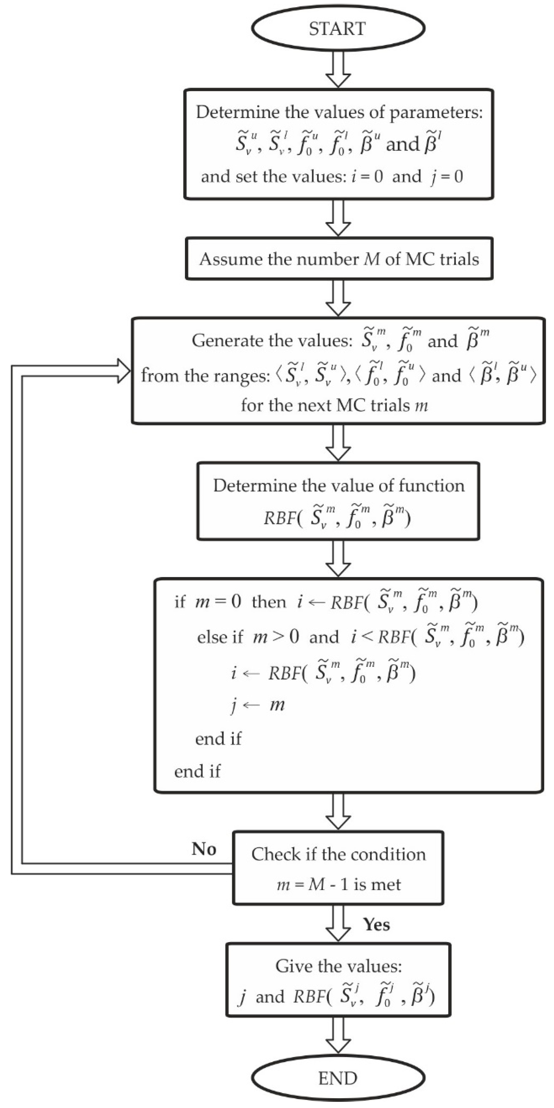
6. MC-Based Procedure for Determining the UAERBF(max)

Let the variables S ˜ V , f ˜ 0 , and β ˜ denote the parameters of the mathematical model of the voltage-mode accelerometer assumed in advance or determined based on the WLS method [33,34], while the variables u ( S ˜ V ) , u ( f ˜ 0 ) , and u ( β ˜ ) are the uncertainties associated with these parameters. Also, let
S ˜ V u = S ˜ V + u ( S ˜ V ) ,   S ˜ V l = S ˜ V u ( S ˜ V ) f ˜ 0 u = f ˜ 0 + u ( f ˜ 0 ) ,   f ˜ 0 l = f ˜ 0 u ( f ˜ 0 ) β ˜ u = β ˜ + u ( β ˜ ) ,   β ˜ l = β ˜ u ( β ˜ )
where ( u ) and ( l ) denote the upper and the lower ranges of the parameter changes by the values of associated uncertainties.
If the R B F was determined on the basis of the accelerometer model parameters for the assumed-in-advance ranges S V , S V + , f 0 , f 0 + , and β , β + , and if the below conditions
S ˜ V u S V , S V + , S ˜ V l S V , S V + f ˜ 0 u f 0 , f 0 + , f ˜ 0 l f 0 , f 0 + β ˜ u β , β + , β ˜ l β , β +
are met, then it is possible to use the MC method to determine such values of the accelerometer model parameters S ˜ V m a x , f ˜ 0 m a x , and β ˜ m a x from the ranges S ˜ V l , S ˜ V u , f ˜ 0 l , f ˜ 0 u , and β ˜ l , β ˜ u , respectively, for which the value of UAERBF(max) is obtained. It is carried out on the basis of R B F ( S ˜ V m a x , f ˜ 0 m a x , β ˜ m a x ) .
Figure 3 shows the block diagram of the MC-based procedure intended for determining the UAERBF(max). The lower number M of the MC trials is calculated based on the formula
M > 10 4 / ( 1 p )
according to the guide [34], where p is the assumed coverage probability. The value of p is usually taken as equal to 0.95. During each MC trial ( m = 0 , M 1 ) , the values of parameters S ˜ V m , f ˜ 0 m , and β ˜ m are generated from the ranges S ˜ V l , S ˜ V u , f ˜ 0 l , f ˜ 0 u , and β ˜ l , β ˜ u , respectively. Based on them, the following value of R B F ( S ˜ V m , f ˜ 0 m , β ˜ m ) is determined. The current maximum value of this function and the corresponding number m of trials are stored in memory (carried out by an assignment of these values to the variables i and j , respectively). For the trial equal to M 1 , the value of R B F ( S ˜ V j , f ˜ 0 j , β ˜ j ) corresponding to the U A E R B F ( m a x ) is determined. The parameters S ˜ V j , f ˜ 0 j and β ˜ j correspond to the parameters defined above by S ˜ V m a x , f ˜ 0 m a x and β ˜ m a x .
Uncertainties associated with the parameters S ˜ V j , f ˜ 0 j and β ˜ j are determined based on the formula
u ( δ ) = 1 M 1 m = 0 M 1 ( δ m δ ¯ ) 2
where
δ ¯ = 1 M m = 0 M 1 δ m
and δ denotes the variable that should be substituted by this parameter of the accelerometer model for which the uncertainty is determined [11,34]. The uncertainty associated with the UAERBF(max) is determined in an analogous way (Figure 3).

7. Results and Verification

Table 1 includes the values of the U A E obtained based on the parameters from the ranges S v 0.100 ,   0.150 and β 0.0100 ,   0.0150 , as well as for the constant value of parameter f 0 equal to 1   kHz .
The quantization steps for the parameters S v and β were equal to 0.002 and 0.0002, respectively. Taking into account the assumptions above, we have S V = 0.100 , S V + = 0.150 , β = 0.0100 , and β + = 0.0150 according to Equation (38). The values of the UAE were obtained by utilizing the algorithm presented in Section 4 for the input parameters: a = S v and T = 0.1   s . The 15th-order Butterworth filter with the cut-off frequency f c was determined by solving the equation describing the amplitude response obtained based on Equation (1).
On the basis of the values of the U A E tabulated in Table 1 and by applying the procedure presented in Section 5, the R B F ( S V , β ) was determined. The cases of 5, 10, and 15 radial neurons based on Equations (28)–(30) were checked.
  • For five radial neurons:
    R B F 5 ( S V , β ) = 36131833920.92137 e 0.020 | ( 0.0134 β ) 2 + ( 0.1400 S V ) 2 | + 11081182573.68980 e 0.020 | ( 0.0114 β ) 2 + ( 0.1260 S V ) 2 | 47491590540.28882 e 0.020 | ( 0.0146 β ) 2 + ( 0.1380 S V ) 2 | + 1065125193.52684 e 0.020 | ( 0.0116 β ) 2 + ( 0.1100 S V ) 2 | + 23506064273.49600 e 0.020 | ( 0.0148 β ) 2 + ( 0.1280 S V ) 2 |
  • For 10 radial neurons:
    R B F 10 ( S V , β ) = 86057837.62482 e 20 | ( 0.0124 β ) 2 + ( 0.1040 S V ) 2 | + 1137987870.37293 e 20 | ( 0.0130 β ) 2 + ( 0.1220 S V ) 2 | + 3414860359.97698 e 20 | ( 0.0128 β ) 2 + ( 0.1280 S V ) 2 | + 426811407.83125 e 20 | ( 0.0142 β ) 2 + ( 0.1140 S V ) 2 | 3260248505.26396 e 20 | ( 0.0132 β ) 2 + ( 0.1280 S V ) 2 | + + 172825594.36315 e 20 | ( 0.0118 β ) 2 + ( 0.1420 S V ) 2 | 1390178.49538 e 20 | ( 0.0100 β ) 2 + ( 0.1060 S V ) 2 | + + 415316898.45332 e 20 | ( 0.0132 β ) 2 + ( 0.1100 S V ) 2 | 243670439.6692 e 20 | ( 0.0116 β ) 2 + ( 0.1400 S V ) 2 | + + 1153163476.99674 e 20 | ( 0.0138 β ) 2 + ( 0.1220 S V ) 2 |
  • For 15 radial neurons:
    R B F 15 ( S V , β ) = 50217932.38037 e 50 | ( 0.0142 β ) 2 + ( 0.1360 S V ) 2 | + 338803095.53718 e 50 | ( 0.0124 β ) 2 + ( 0.1160 S V ) 2 | 99592530.74858 e 50 | ( 0.0124 β ) 2 + ( 0.1040 S V ) 2 | + + 1438055151.11707 e 50 | ( 0.0126 β ) 2 + ( 0.1240 S V ) 2 | 15000132.12083 e 50 | ( 0.0100 β ) 2 + ( 0.1460 S V ) 2 | + 19539648.46192 e 50 | ( 0.0148 β ) 2 + ( 0.1480 S V ) 2 | + 19065043.38108 e 50 | ( 0.0138 β ) 2 + ( 0.1480 S V ) 2 | + + 229678117.86818 e 50 | ( 0.0110 β ) 2 + ( 0.1260 S V ) 2 | + 166603554.85264 e 50 | ( 0.0132 β ) 2 + ( 0.1080 S V ) 2 | + 777217752.67323 e 50 | ( 0.0124 β ) 2 + ( 0.1280 S V ) 2 | 665634775.90997 e 50 | ( 0.0120 β ) 2 + ( 0.1240 S V ) 2 | + 112930795.30634 e 50 | ( 0.0150 β ) 2 + ( 0.1200 S V ) 2 | + 67735452.91154 e 50 | ( 0.0110 β ) 2 + ( 0.1380 S V ) 2 | + + 3949404.8155 e 50 | ( 0.0102 β ) 2 + ( 0.1020 S V ) 2 | + 53414134.78681 e 50 | ( 0.0110 β ) 2 + ( 0.1060 S V ) 2 |
Computational experiments were carried out for three given network structures with different hidden layer parameters and including sizes of 5, 10, and 15 neurons. Optimal hyperparameters and relevant criteria (statistical measures) regarding the quality of the model were calculated in each experiment. The obtained results are presented in Table 2, where Max error, MSE, MAE, MedAE, and R2 denote the maximum error, mean squared error, mean absolute error, median absolute error, and determination coefficient, respectively.
For the functions above, the coefficient R 2 was equal to 0.997300, 0.999970, and 0.999998, respectively. In turn, the values of MSE were: 1.27 × 10 4 , 1.39 × 10 6 , and 9.94 × 10 8 ,   respectively. For comparison, in the case of polynomial approximation presented in [18], the MSE was equal to 1.66 and 0.31, while in the case of using this approximation in [19], the fitting coefficient was equal to 0.797. Thus, it can easily be concluded that the fitting indexes obtained by the RBF are significantly better than those obtained with applying the polynomial approximation. In the case of 15 neurons, the values of UAERBF obtained by substitution of the parameters S V and β from Table 1 into the R B F 15 ( S V , β ) were, in most cases, the same as the values of the UAE tabulated in this table.
Figure 4a–d shows the values of the UAE tabulated in Table 1 and an approximation of the UAE using the RBF according to Equations (28)–(30).
The abovementioned approximation approach was implemented using Python 3.6 [40] and computed on a hardware configuration that included an Intel Core i5 M430, 2.27 GHz, 8 MB RAM and the operating system Windows 7 to obtain the experimental results. The following Python-related scientific packages were used in the implementation: NumPy, SciPy, iPython, Scikit-learn, Pandas, and Matplotlib for visualization purposes [41,42,43,44,45].
The values of UAERBF determined based on R B F 15 ( S V , β ) for the values of parameters S ˜ V and β ˜ selected from the ranges S V , S V + and β , β + are shown in Table 3.
Let us assume that the uncertainties associated with the parameters S ˜ V and β ˜ included in Table 3 are: u ( S ˜ V ) = 0.001 and u ( β ˜ ) = 0.0001 , respectively. In this case, according to Equation (23), we have S ˜ V u = 0.150 , S ˜ V l = 0.100 , β ˜ u = 0.0150 , and β ˜ l = 0.0100 . The conditions given by Equation (24) are therefore met. Hence, we can use the MC method based on the Wichmann–Hill pseudorandom number generator to determine the parameters S ˜ V m a x and β ˜ m a x , which produce the U A E R B F ( m a x ) . For p = 0.95 , the minimum number M of MC trials equal to 2 × 10 5 , obtained based on Equations (25), was applied for the calculations below.
The results of the MC simulation, tabulated in Table 4, are shown in the following order: UAERBF(max) , S ˜ V m a x ± u ( S ˜ V m a x ) , β ˜ m a x ± u ( β ˜ m a x ) , and the number m of the corresponding MC trial.
Based on the obtained results, it can be easily concluded that, in most cases, the values of parameters S ˜ V m a x and β ˜ m a x were contained in the ranges S V , S V + and β , β + . It confirms the advisability of using the MC method to determine them. This is the only correct way to accurately determine the parameters of a voltage-mode accelerometer, which produce the U A E R B F ( m a x ) . When assuming the variability of all three parameters of the accelerometer, the functions of three variables are obtained, similar to those presented by Equations (28). When the values of parameters with associated uncertainties are obtained based on the WLS method, then the values of the parameters S ˜ V m a x , f ˜ 0 m a x , and β ˜ m a x and the value of UAERBF(max) are determined using the MC method in an analogous way to that above.

8. Conclusions

This paper presents the procedure for determining the RBF based on the numerical values of the UAE calculated for a voltage-mode accelerometer as an example. These UAEs were determined for the both the assumed-in-advance ranges of variability of the parameters of the accelerometer model and the quantization steps of these parameters. When the RBF is obtained in this way, we can easily and quickly calculate the UAE for any values of the parameters of an accelerometer model from the ranges above. The error obtained in this way is denoted by UAERBF. The above facility results from the fact that it is not always necessary to use the algorithm dedicated to determinining the UAE and the related necessity of determining the cut-off frequency of the standard applied as a reference for calculating the error.
The paper also discussed in detail the use of the MC method to determine the UAE (such error is denoted by UAERBF(max)) when considering the uncertainties associated with the parameters of an accelerometer model. To ensure the correct realization of the procedures for modeling a voltage-mode accelerometer by applying the parametric identification, such uncertainties should always be determined. The MC method is based on the previously determined RBFs for such ranges of change in the parameters of the accelerometer model, which contain all parameters for the accelerometer considered in a particular case. It is also important to underline that the parameters of such accelerometer, in the case of their decrease or increase by the values of the uncertainties associated with them, do not go beyond the lower and upper limits of the parameters for which the RBF was earlier determined.
The solutions presented in this paper regarding the determination of the RBF using an RBF-NN for an assumed number of radial neurons and the application of the MC method for determining the UAERBF(max) are the first solutions in the subject of measurement traceability. Based on the results obtained for the solutions above, in the case of 15 radial neurons, it can be seen that the statistical ratios regarding the uncertainty of approximation of the values of UAE using the RBF are much higher than those obtained using the polynomial approximation presented in [18] and [19]. The obtained values of these ratios also confirm that the number of neurons equal to 15 is optimal in terms of the uncertainty of an approximation of the UAE using the RBF.
The RBFs for the assumed range of variability of two accelerometer parameters were determined in this paper. This assumption was required to limit the number of calculation results intended for the presentation here. However, based on the displayed procedures, the RBF can be easily determined for the assumed ranges of variability of all three parameters of the accelerometer model.
Based on the obtained low uncertainty of the approximation for 15 neurons, it can be concluded that the RBFs determined for such a number of neurons can be successfully applied for the mutual comparison of the UAERBF(max) obtained for different types of accelerometers. It should be kept in mind, however, that the compared accelerometers should have the same frequency bandwidth of operation and that the parameters associated with their models must be within the ranges of parameter changes for which the RBF was determined.

Author Contributions

Conceptualization, K.T. and M.P.; data curation, M.P. and G.S.; writing—original draft, K.T. and M.P.; formal analysis, K.T. and M.P.; methodology, K.T. and M.P.; writing—review and editing, G.S.; software, K.T. and M.P.

Funding

This research was funded under the grant numbers BS-207/M/2019 (Pedagogical University of Cracow statutory research grant) and E-3/563/2018/DS (Cracow University of Technology), was funded by subsidies for science granted by the Polish Ministry of Science and Higher Education.

Conflicts of Interest

The authors declare no conflict of interest.

References

  1. Ghemari, Z.; Salah, S.; Abdelwaheb, A.; Lakehal, A. New Model of Piezoelectric Accelerometer Relative Movement Modulus. Trans. Inst. Meas. Control 2014, 58, 707–712. [Google Scholar]
  2. Sun, X.T.; Jing, X.J.; Xu, J.; Cheng, L. A Quasi-Zero-Stiffness-Based Sensor System in Vibration Measurement. IEEE Trans. Ind. Electron. 2014, 61, 5606–6114. [Google Scholar]
  3. Sharapov, V. Piezoceramic Sensors; Springer: Berlin/Heidelberg, Germany, 2011. [Google Scholar]
  4. BIPM; IEC; IFCC; ILAC; ISO; IUPAC; IUPAP; OIML. International Vocabulary of Metrology—Basic and General Concepts and Associated Terms (VIM), 3rd ed. Available online: https://www.bipm.org/utils/common/documents/jcgm/JCGM_200_2012.pdf (accessed on 24 September 2019).
  5. Prajapati, H.; Deshmukh, N.N. Design and development of thin wire sensor for transient temperature measurement. Measurement 2019, 140, 582–589. [Google Scholar]
  6. Sabuga, W.; Rabault, T.; Wüthrich, C.; Pražák, D.; Chytil, M.; Brouwer, L.; Ahmed, A.D.S. High pressure metrology for industrial applications. Metrologia 2017, 54, 27–44. [Google Scholar]
  7. Wilczynska, T.; Wisniewski, R.; Konarski, P. Temperature and pressure properties of the resistance alloy ZERANIN30 implanted by high dose, middle energy, C+ ions. Prz. Elektrotech. 2012, 88, 292–295. [Google Scholar]
  8. Sulowicz, M.; Ludwinek, K.; Tulicki, J.; Depczynski, W.; Nowakowski, L. Practical adaptation of a low-cost voltage transducer with an open feedback loop for precise measurement of distorted voltages. Sensors 2019, 19, 1071. [Google Scholar] [CrossRef]
  9. Layer, E. Theoretical Principles for Establishing a Hierarchy of Dynamic Accuracy with the Integral-Square-Error as an Example. IEEE Trans. Instrum. Meas. 1997, 46, 1178–1182. [Google Scholar]
  10. Omer, A.I.; Taleb, M.M. Measurement Systems: Characteristics and Models. Eur. Sci. J. 2014, 10, 248–260. [Google Scholar]
  11. BIPM; IEC; IFCC; ILAC; ISO; IUPAC; IUPAP; OIML. Supplement 2 to the Guide to the Expression of Uncertainty in Measurement—Extension to any Number of Output Quantities. Available online: https://www.bipm.org/utils/common/documents/jcgm/JCGM_102_2011_E.pdf (accessed on 24 September 2019).
  12. Layer, E.; Gawedzki, W. Theoretical principles for dynamic errors measurement. Measurement 1990, 8, 45–48. [Google Scholar]
  13. Shestakov, A.L. Dynamic measuring methods: A review. Acta IMEKO 2019, 8, 64–76. [Google Scholar]
  14. Hessling, J.P. A novel method of estimating dynamic measurement errors. Meas. Sci. Technol. 2006, 17, 173–182. [Google Scholar]
  15. Dichev, D.; Koev, H.; Bakalova, T.; Louda, P. A Model of the Dynamic Error as a Measurement Result of Instruments Defining the Parameters of Moving Objects. Meas. Sci. Rev. 2014, 14, 183–189. [Google Scholar] [Green Version]
  16. Honig, M.L.; Steiglitz, K. Maximizing the output energy of a linear channel with a time and amplitude limited input. IEEE Trans. Inf. Theory 1992, 38, 1041–1052. [Google Scholar]
  17. Tomczyk, K.; Layer, E. Accelerometer errors in measurements of dynamic signals. Measurement 2015, 60, 292–298. [Google Scholar]
  18. Tomczyk, K. Polynomial approximation of the maximum dynamic error generated by measurement systems. Prz. Elektrotech. 2019, 95, 124–127. [Google Scholar]
  19. Tomczyk, K. New algorithm for determining the dynamic error for the integral-square criterion. J. Phys. Conf. Ser. 2018, 1065, 1–4. [Google Scholar]
  20. Rutland, N.K. The principle of matching: Practical conditions for systems with inputs restricted in magnitude and rate of change. IEEE Trans. Automat. Control 1994, 39, 550–553. [Google Scholar]
  21. Tomczyk, K. Levenberg-Marquardt Algorithm for Optimization of Mathematical Models according to Minimax Objective Function of Measurement Systems. Metrol. Meas. Syst. 2009, 16, 599–606. [Google Scholar]
  22. Curve Fitting Toolbox. Available online: http://cda.psych.uiuc.edu/matlab_pdf/curvefit.pdf (accessed on 26 August 2019).
  23. Sinha, P. Multivariate Polynomial Regression in Data Mining: Methodology, Problems and Solutions. J. Sci. Eng. Res. 2013, 4, 962–965. [Google Scholar]
  24. Rady El-Housseiny, A.; Ziedan, D. Estimation of Population Total Using Local Polynomial Regression with Two Auxiliary Variables. J. Stat. Appl. Probab. 2014, 2, 129–136. [Google Scholar]
  25. Neural Network Toolbox. Available online: http://cda.psych.uiuc.edu/matlab_pdf/nnet.pdf (accessed on 26 August 2019).
  26. Dudzik, M.; Tomczyk, K.; Jagiello, A.S. Analysis of the error generated by the voltage output accelerometer using the optimal structure of an artificial neural network. In Proceedings of the 2018 19th International Conference on Research and Education in Mechatronics (REM 2018), Delft, The Netherlands, 7–8 June 2018; pp. 7–11. [Google Scholar]
  27. Dudzik, M.; Tomczyk, K.; Sieja, M. Optimal dynamic error formula for charge output accelerometer obtained by the neural network. In Proceedings of the International Symposium on Electrical Machines (SME 2018), Andrychow, Poland, 10–13 June 2018; pp. 1–4. [Google Scholar]
  28. Park, J.; Sandberg, I.W. Universal Approximation Using Radial-Basis-Function Networks. Neural Comput. 1991, 3, 246–257. [Google Scholar] [PubMed]
  29. Buljak, V.; Maier, G. Proper orthogonal decomposition and radial basis functions in material characterization based on instrumented indentation. Eng. Struct. 2011, 33, 492–501. [Google Scholar]
  30. Buljak, V. Proper orthogonal decomposition and radial basis functions algorithm for diagnostic procedure based on inverse analysis. FME Trans. 2010, 38, 129–136. [Google Scholar]
  31. Benaissa, B.; Köppen, M.; Wahab, M.A.; Khatir, S. Application of proper orthogonal decomposition and radial basis functions for crack size estimation using particle swarm optimization. J. Phys. Conf. Ser. 2017, 842, 1–11. [Google Scholar]
  32. Xiao, D.; Fang, F.; Pain, C.C.; Navon, I.M.; Salinas, P.; Muggeridge, A. Non-intrusive reduced order modeling of multi-phase flow in porous media using the POD-RBF method. J. Comput. Phys. 2015, 1, 1–25. [Google Scholar]
  33. Link, A.; Täbner, A.; Wabinski, W.; Bruns, T.; Elster, C. Modelling accelerometers for transient signals using calibration measurement upon sinusoidal excitation. Measurement 2007, 40, 928–935. [Google Scholar]
  34. BIPM; IEC; IFCC; ILAC; ISO; IUPAC; IUPAP; OIML. Evaluation of Measurement Data—Supplement 1 to the Guide to the Expression of Uncertainty in Measurement—Propagation of Distributions Using a Monte Carlo Method. Available online: https://www.bipm.org/utils/common/documents/jcgm/JCGM_101_2008_E.pdf (accessed on 24 September 2019).
  35. Guimarães Couto, P.R.; Carreteiro Damasceno, J.; de Oliveira, S.P. Monte Carlo Simulations Applied to Uncertainty in Measurement; IntechOpen: London, UK, 2013; pp. 27–51. [Google Scholar]
  36. Harris, P.M.; Cox, M.G. On a Monte Carlo method for measurement uncertainty evaluation and its implementation. Metrologia 2014, 51, 176–182. [Google Scholar]
  37. Wichmann, B.A.; Hill, I.D. Generating Good Pseudo-Random Numbers. Comput. Stat. Data Anal. 2006, 51, 1614–1622. [Google Scholar]
  38. Strang, G. Linear Algebra and its Applications, 2nd ed.; Academic Press Inc.: Orlando, FL, USA, 1980; pp. 139–142. [Google Scholar]
  39. Python Software Foundation. Python Language Reference, Version 3.6. Available online: http://www.python.org (accessed on 26 August 2019).
  40. Hunter, J.D. Matplotlib: A 2D Graphics Environment. Comput. Sci. Eng. 2007, 9, 90–95. [Google Scholar]
  41. Pedregosa, F.; Varoquaux, G.; Gramfort, A.; Michel, V.; Thirion, B.; Grisel, O.; Blondel, M.; Prettenhofer, P.; Weiss, R.; Dubourg, V.; et al. Scikit-learn: Machine Learning in Python. J. Mach. Learn. Res. 2011, 12, 2825–2830. [Google Scholar]
  42. Van der Walt, S.; Colbert, S.C.; Varoquaux, G. The NumPy Array: A Structure for Efficient Numerical Computation. Comput. Sci. Eng. 2011, 13, 22–30. [Google Scholar] [Green Version]
  43. McKinney, W. Data Structures for Statistical Computing in Python. In Proceedings of the 9th Python in Science Conference, Austin, TX, USA, 28 June–3 July 2010; Volume 445, pp. 51–56. [Google Scholar]
  44. Pérez, F.; Granger, B.E. IPython: A System for Interactive Scientific Computing. Comput. Sci. Eng. 2007, 9, 21–29. [Google Scholar]
  45. Jones, E.; Oliphant, E.; Peterson, P. SciPy: Open Source Scientific Tools for Python 2001. Available online: http://www.scipy.org (accessed on 26 August 2019).
Figure 1. Block diagram of the procedure intended for determining the radial basis function (RBF) and the value of absolute dynamic error (UAERBF).
Sensors 19 04154 g001
Figure 2. Block diagram of the procedure intended for determining the UAERBF(max).
Sensors 19 04154 g002
Figure 3. Block diagram of the Monte Carlo (MC)-based procedure for determining the UAERBF(max).
Sensors 19 04154 g003
Figure 4. Visualization of the approximation surfaces obtained (blue wireframe), where original input dataset values are marked in red: (a) Original data, (b) surface mapped with 5 neurons, (c) surface mapped with 10 neurons, and (d) surface mapped with 15 neurons.
Sensors 19 04154 g004
Table 1. Values of the UAE.
β
0.01000.01020.01040.01060.01080.01100.01120.01140.01160.01180.01200.01220.0124
S v 0.1000.6340.6210.6100.5980.5870.5760.5660.5560.5470.5370.5280.5200.511
0.1020.6600.6470.6340.6220.6110.6000.5890.5790.5690.5590.5500.5410.532
0.1040.6860.6720.6590.6470.6350.6230.6120.6020.5910.5810.5710.5620.553
0.1060.7120.6980.6850.6720.6590.6480.6360.6250.6140.6040.5940.5840.575
0.1080.7390.7250.7110.6980.6850.6720.6600.6490.6380.6270.6160.6060.596
0.1100.7670.7520.7380.7240.7100.6970.6850.6730.6610.6500.6390.6290.619
0.1120.7950.7800.7650.7500.7360.7230.7100.6980.6860.6740.6630.6520.641
0.1140.8240.8080.7920.7770.7630.7490.7360.7230.7100.6980.6870.6750.664
0.1160.8530.8360.8200.8050.7900.7760.7620.7480.7350.7230.7110.6990.688
0.1180.8830.8650.8490.8330.8170.8030.7880.7740.7610.7480.7360.7240.712
0.1200.9130.8950.8780.8610.8450.8300.8150.8010.7870.7740.7610.7480.736
0.1220.9430.9250.9070.8900.8740.8580.8430.8280.8130.8000.7860.7730.761
0.1240.9750.9560.9370.9200.9020.8860.8700.8550.8400.8260.8120.7990.786
0.1261.0060.9870.9680.9500.9320.9150.8990.8830.8680.8530.8390.8250.812
0.1281.0391.0180.9990.9800.9620.9440.9270.9110.8950.8800.8660.8510.838
0.1301.0711.0501.0301.0110.9920.9740.9570.9400.9240.9080.8930.8780.864
0.1321.1041.0831.0621.0421.0231.0040.9860.9690.9520.9360.9210.9050.891
0.1341.1381.1161.0951.0741.0541.0351.0160.9990.9810.9650.9490.9330.918
0.1361.1721.1491.1281.1061.0861.0661.0471.0291.0110.9940.9770.9610.946
0.1381.2071.1831.1611.1391.1181.0981.0781.0591.0411.0231.0060.9900.974
0.1401.2421.2181.1951.1721.1501.1301.1091.0901.0711.0531.0361.0191.002
0.1421.2781.2531.2291.2061.1831.1621.1411.1211.1021.0831.0651.0481.031
0.1441.3141.2891.2641.2401.2171.1951.1741.1531.1331.1141.0961.0781.060
0.1461.3511.3251.3001.2751.2511.2291.2071.1851.1651.1451.1261.1081.090
0.1481.3881.3611.3351.3101.2861.2621.2401.2181.1971.1771.1571.1381.120
0.1501.4261.3981.3721.3461.3211.2971.2741.2511.2301.2091.1891.1691.150
β
0.01260.01280.01300.01320.01340.01360.01380.01400.01420.01440.01460.01480.0150
S v 0.1000.5030.4950.4880.4800.4730.4660.4590.4530.4470.4400.4340.4280.423
0.1020.5240.5150.5070.5000.4920.4850.4780.4710.4650.4580.4520.4460.440
0.1040.5440.5360.5280.5200.5120.5040.4970.4900.4830.4760.4700.4630.457
0.1060.5650.5570.5480.5400.5320.5240.5160.5090.5020.4950.4880.4810.475
0.1080.5870.5780.5690.5600.5520.5440.5360.5280.5210.5140.5070.5000.493
0.1100.6090.5990.5900.5810.5730.5640.5560.5480.5400.5330.5260.5180.512
0.1120.6310.6210.6120.6030.5940.5850.5760.5680.5600.5520.5450.5370.530
0.1140.6540.6440.6340.6240.6150.6060.5970.5890.5800.5720.5640.5570.549
0.1160.6770.6670.6560.6460.6370.6270.6180.6090.6010.5930.5840.5770.569
0.1180.7010.6900.6790.6690.6590.6490.6400.6310.6220.6130.6050.5970.589
0.1200.7250.7130.7020.6920.6810.6710.6620.6520.6430.6340.6250.6170.609
0.1220.7490.7370.7260.7150.7040.6940.6840.6740.6650.6550.6460.6380.629
0.1240.7740.7620.7500.7390.7280.7170.7060.6960.6870.6770.6680.6590.650
0.1260.7990.7860.7740.7630.7510.7400.7290.7190.7090.6990.6900.6800.671
0.1280.8240.8120.7990.7870.7750.7640.7530.7420.7320.7220.7120.7020.693
0.1300.8500.8370.8240.8120.8000.7880.7760.7650.7550.7440.7340.7240.714
0.1320.8770.8630.8500.8370.8240.8120.8010.7890.7780.7670.7570.7470.737
0.1340.9040.8890.8760.8620.8500.8370.8250.8130.8020.7910.7800.7690.759
0.1360.9310.9160.9020.8880.8750.8620.8500.8380.8260.8150.8030.7930.782
0.1380.9580.9430.9290.9150.9010.8880.8750.8620.8500.8390.8270.8160.805
0.1400.9860.9710.9560.9410.9270.9140.9010.8880.8750.8630.8510.8400.829
0.1421.0150.9990.9830.9690.9540.9400.9260.9130.9000.8880.8760.8640.852
0.1441.0431.0271.0110.9960.9810.9670.9530.9390.9260.9130.9010.8880.877
0.1461.0731.0561.0401.0241.0090.9940.9790.9650.9520.9390.9260.9130.901
0.1481.1021.0851.0681.0521.0361.0211.0060.9920.9780.9650.9510.9390.926
0.1501.1321.1141.0971.0811.0651.0491.0341.0191.0050.9910.9770.9640.951
Table 2. Summary of model quality assessment for various hidden layer sizes.
Number of NeuronsMax Error (%)MSEMAEMedAER2
52.6801.27 × 10−40.009400.008600.997300
100.3101.39 × 10−60.000980.000930.999970
150.0989.94 × 10−80.000240.000170.999998
Table 3. Values of the UAERBF for the selected values of parameters S ˜ V and β ˜ .
β ˜
0.01010.01170.01330.0149
S ˜ V 0.1010.6410.5520.4870.434
0.1170.8590.7420.6530.582
0.1331.110.9590.8430.753
0.1491.3921.2041.0580.945
Table 4. Results of MC simulation.
β ˜ ± u ( β ˜ )
0.01010 ± 0.00001 0.01170 ± 0.00001 0.01330 ± 0.00001 0.01490 ± 0.00001
S ˜ V ± u ( S ˜ V ) 0.1010 ± 0.0001 0.643
1011 · 10 4 ± 3 · 10 9
1009 · 10 5 ± 4 · 10 11
133,864
0.554
1010 · 10 4 ± 6 · 10 9
1169 · 10 5 ± 5 · 10 11
95,693
0.488
1011 · 10 4 ± 7 · 10 9
1329 · 10 5 ± 8 · 10 11
77,444
0.435
1012 · 10 4 ± 2 · 10 9
1489 · 10 5 ± 3 · 10 11
47,515
0.1170 ± 0.0001 0.862
1171 · 10 4 ± 9 · 10 9
1009 · 10 5 ± 2 · 10 11
17,202
0.744
1171 · 10 4 ± 7 · 10 9
1169 · 10 5 ± 3 · 10 11
75,560
0.654
1171 · 10 4 ± 6 · 10 9
1329 · 10 5 ± 3 · 10 11
23,843
0.584
1171 · 10 4 ± 3 · 10 9
1489 · 10 5 ± 3 · 10 11
46,042
0.1330 ± 0.0001 1.110
1131 · 10 4 ± 2 · 10 9
1009 · 10 5 ± 5 · 10 11
166,502
0.961
1331 · 10 4 ± 3 · 10 9
1169 · 10 5 ± 7 · 10 11
194,645
0.845
1331 · 10 4 ± 1 · 10 9
1329 · 10 5 ± 4 · 10 11
70,163
0.755
1331 · 10 4 ± 3 · 10 9
1329 · 10 5 ± 4 · 10 11
175,809
0.1490 ± 0.0001 1.401
1491 · 10 4 ± 3 · 10 9
1009 · 10 5 ± 6 · 10 11
181,360
1.210
1491 · 10 4 ± 2 · 10 9
1169 · 10 5 ± 5 · 10 11
121,431
1.062
1491 · 10 4 ± 3 · 10 9
1329 · 10 5 ± 8 · 10 11
76,186
0.947
1491 · 10 4 ± 4 · 10 9
1489 · 10 5 ± 2 · 10 11
94,832

