Geophonino-W: A Wireless Multichannel Seismic Noise Recorder System for Array Measurements

 ,
,  ,
, 
Abstract
1. Introduction
2. System Development and Implementation
2.1. General
- When accessibility to the desired location of the sensors is complicated, and the whole setup has to be established in-situ.
- In array measurements, when the deployment of several sensors, especially those with large apertures, may make the connection of the sensors with the recorder extremely difficult and even more difficult, if these measures are carried out in urban areas.
- In ambient noise measurements of buildings, in which their dynamic characteristics, such as their natural frequencies and mode shapes, may be evaluated [18].
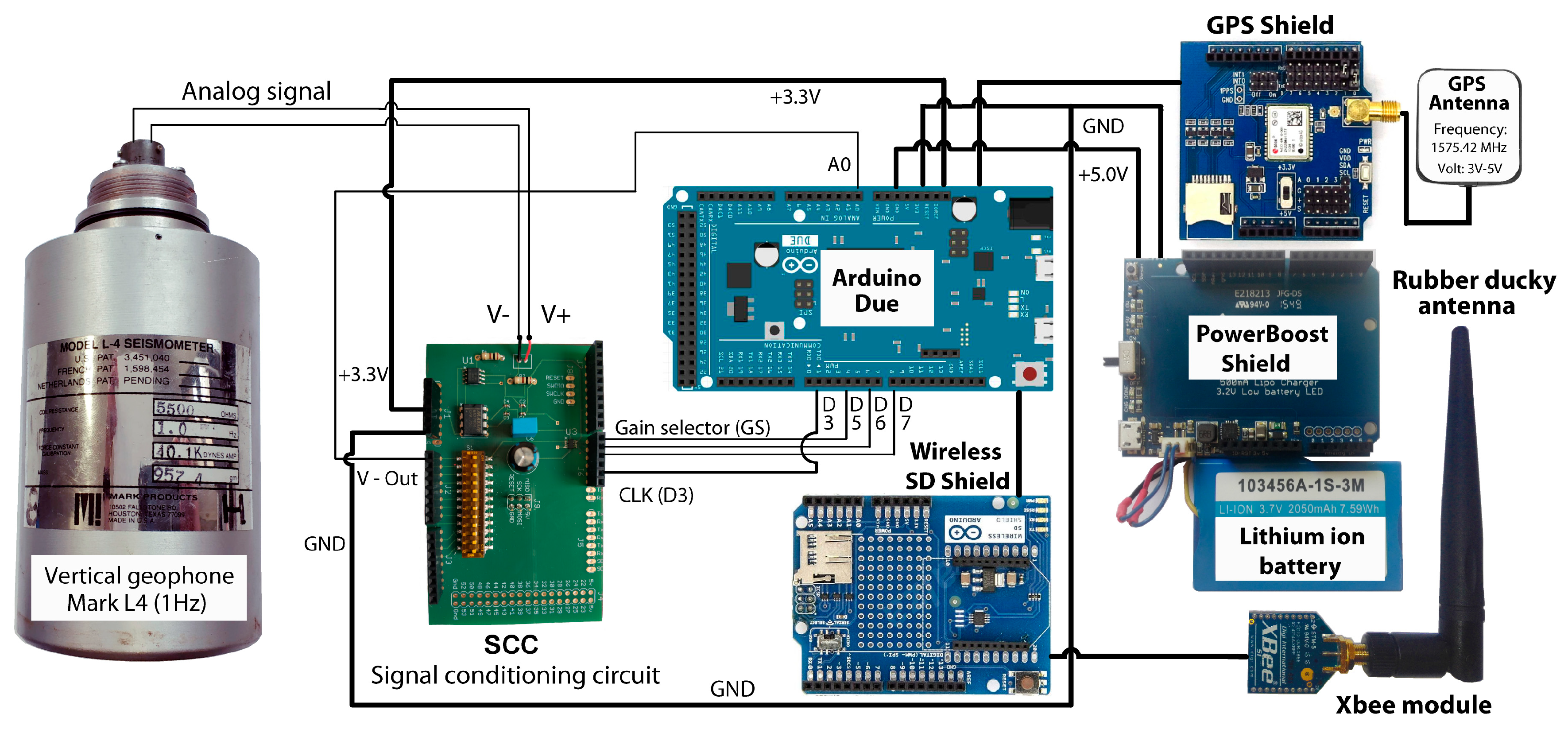
2.2. System Hardware
- An Arduino Due board;
- A DS3231 Precision RTC (Real time clock), with a 3 V CR1220 40 mAh battery;
- An Arduino Wireless SD Shield, with an 8 Gb SD card;
- An Xbee S1 802.15.4 low-power module, with an RPSMA connector;
- A 2.4 GHz omnidirectional rubber ducky antenna, model HG2403RD, with a gain of 3 dBi (decibels relative to the isotropic).
- An Arduino Due board;
- An Arduino Wireless SD Shield, with an 8 Gb SD card;
- An Xbee S1 802.15.4 low-power module, with an RPSMA connector;
- A 2.4 GHz omnidirectional rubber ducky antenna, model HG2403RD, with a gain of 3 dBi (decibels relative to isotropic);
- An ITEAD RoyalTek REB-5216 GPS Shield Breakout Board;
- A GPS active antenna, model IM120717003;
- A PowerBoost shield adapter, with an output of 5 V 500 mA;
- A Lithium ion 3.7 V 2050 mAh rechargeable battery, model 103456A-1S-3M;
- A Signal Conditioning Circuit (SCC).
2.3. System Communications
- (1)
- Selection of the API mode. In the serial interfacing options, the AP parameter is changed to “AP-enabled w/PPP”.
- (2)
- Definition of a common network. In order to allow for communication among all the Xbee modules, they have to be included in the same network. To achieve this, the Pan ID parameter is set up with the same value for all nodes. In our case, the 855 value has been selected.
- (3)
- Definition of the ACN and MCN addresses. A 16-bit source parameter has to be defined for each component of the wireless network. In our case, the ACN devices have been numbered from 1 to 12, and the MCN module has been labeled with the number 13. By default, the system has been designed for a maximum of 12 ACN devices, but it can easily be modified, with minor changes to the Arduino Due code.
2.4. Design and Implementation of the System Software
2.4.1. MCN Software Implementation
- Identifying the ACN modules within the arrayIn the first step, the MCN assigns a different identification number to each one of the ACN modules integrated in the array of sensors. This identification number is sent to each of the ACN modules and used subsequently in all the communications between the MCN and the ACNs.
- Requesting GPS information from all the ACN modulesIf any of the stations did not respond at least once to the requests, it is discarded for the rest of the operations.
- Sending configuration packets to the ACN modulesThe MCN sends the configuration packets to the different ACN modules. The correct sending of data is controlled through an error communication counter (ECC), which the MCN module activates for each ACN at the beginning of the process. In this way, if the MCN module did not receive any response from any of the ACN modules after 40 attempts (i.e., the ECC reaches the value of 40), then those ACNs would be marked as inactive stations and would not receive further communication attempts from the MCN. The data validation is conducted in the respective ACN modules, which respond to the MCN with a confirmation packet, if everything is correct. If any error was detected, the ACN would respond with an error packet, and the MCN would re-send the configuration packet.
- Synchronizing the internal clock of each ACN module with the MCN clockArray measurements require that all of the stations in the array register simultaneously, so a precise synchronization is required between all the stations [11]. Thus, one of the most important tasks of the MCN is to ensure the strict synchronization between ACNs. The implemented synchronization process is carried out in three main steps. Firstly, the MCN sends a message to each of the ACN modules and waits to receive the answer from the corresponding ACN, measuring the associated travel time. This is repeated twice. The aim is to ensure that the travel times are the same for all of the ACN modules. In the second step, the MCN module calculates the time, in milliseconds, that remains to start the data acquisition. This time is taken as a reference time and should be at least longer than 20 seconds, as this is approximately the time required to synchronize the 12 stations used in this work. Finally, the MCN module asks each ACN for the value of its internal clock, in milliseconds. In this way, taking as the reference time the one calculated in the second step, the time at which the data acquisition should start in each of the ACN modules is obtained and sent to each of them.
- Reading acquisition confirmation packets from the ACN modulesDuring the data acquisition process, each one of the ACN modules sends an acquisition confirmation packet to the MCN every 3 seconds. In this way, if any problem occurred in any of the remote stations (e.g., low battery), then the MCN would detect the ACN that fails. Anyway, the data acquisition would continue with the available active ACN modules.
2.4.2. ACN Software Implementation
- Identification of the array stations: {Message ID = 00, Station ID = 01, 02 … 12}All of the ACN modules are programmed identically. Therefore, in the first step, each of the ACN modules has to be identified within the array. To achieve this, the MCN assigns a different Station ID for each of the ACN modules (i.e., Station ID = 01, 02 … 12) and sends the corresponding identification to each of them. From now on, the Station ID parameter is included in all the messages between the MCN and ACN for identification purposes.
- Sending GPS information to the MCN module: {Message ID = 01, Station ID = 01, 02 … 12}The MCN module uses this Message ID to request GPS information from each of the ACN modules. When one ACN receives this Xbee packet, the program reads and decodes an NMEA GPS trace. The management of the NMEA GPS data packets has been carried out using the TinyGPS (GPL) library [28].Once the GPS information is obtained correctly, the ACN sets its internal RTC with the obtained date and time. Besides, the GPS data are sent to the MCN via the Xbee connection and saved in the SD memory card of the corresponding ACN. The GPS information is saved in an ASCII file, whose name is composed of the time and the date, and the extension is formed by the letter ‘g’, plus the Station ID (e.g., ‘140512_05022019.g01’). This file contains two header lines. The first line contains the Station ID, and the second line contains the description of the saved parameters, that is: Time, Latitude, Longitude, HDOP (Horizontal Dilution Of Precision), and NumSatellites. The HDOP information includes the Horizontal Dilution Of Precision, and NumSatellites includes the number of satellites used to determine the position. This information is provided for each GPS trace.
- Receiving and saving configuration data: {Message ID = 02, Station ID = 01, 02 … 12, Data}This Xbee packet contains all the configuration parameters required for the data acquisition. When this packet is received, the ACN system extracts the different configuration values and saves them in the corresponding local variables of the program. After that, the ACN module sends an Xbee packet to the MCN, indicating whether all of the configuration parameters are correct (confirmation packet) or not (error packet).
- Sending the synchronization packets to the MCN: {Message ID = 03, Station ID = 01, 02 … 12}When any of the ACN modules receives an Xbee packet with a Message ID equaling 3, the associated ACN automatically returns a confirmation packet to the MCN, which is in charge of measuring the travel time between MCN and ACN. This process is repeated twice for each of the ACN modules in order to verify that the travel times are the same for all of them.
- Sending the internal clock to the MCN: {Message ID = 04, Station ID = 01, 02 … 12}When any of the ACN modules receives a Message ID equaling 4, the associated ACN automatically returns its internal clock (in milliseconds) to the MCN, which estimates the time at which the data acquisition should start in that ACN module.
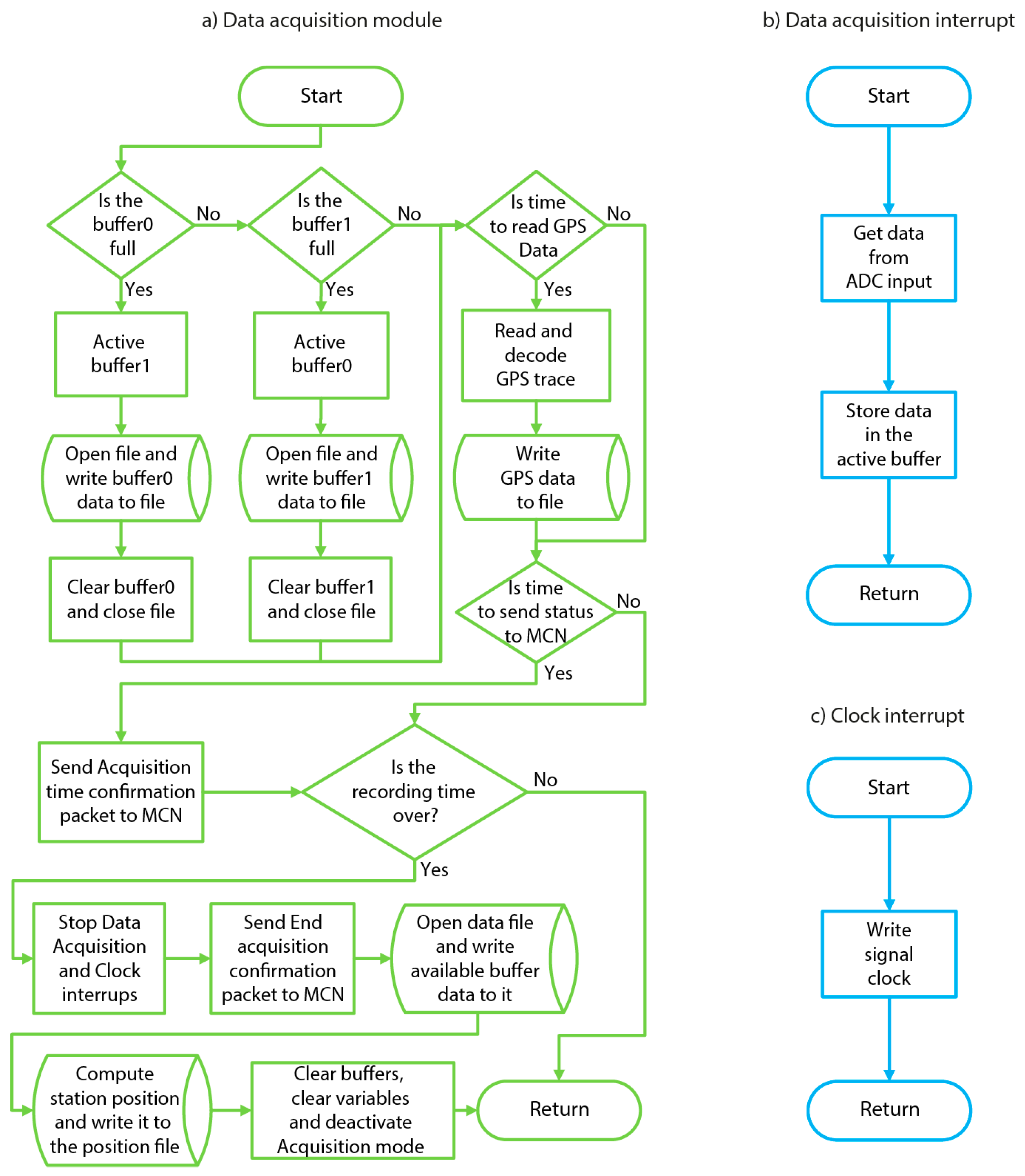
- Starting data acquisition in the millisecond: {Message ID = 05, Station ID = 01, 02 … 12, T}This Xbee packet contains the time (in milliseconds) that it has to reach the associated ACN module, before starting the data acquisition (“Data acquisition” module). During the data acquisition, two interrupts are used. The Data Acquisition Interrupt process uses an Interrupt Service Routine (ISR), which ensures that the samples are acquired at the precise sampling period selected by the user. The Clock Interrupt routine is used to send a signal clock to the MAX7404 (see Section 2.2), which establishes the cut-off frequency of the anti-aliasing filter. In the proposed system, the available sampling frequencies are 100 Hz, 250 Hz and 500 Hz, and the corresponding cut off frequencies are 40 Hz, 100 Hz and 200 Hz, respectively. In Figure 11, a detailed flowchart of the program associated with the “Data acquisition” module, as well as the two interrupts used, is shown.
- Dumping the memory buffers on the SD card. When either of the two buffers are full, the other buffer is automatically activated, and the data are saved in the SD card. The data file is opened and closed in each buffer dump operation. In this way, in case of an unexpected stop of the data acquisition, all of the data are saved, until the moment of the unexpected stop. This is an important improvement in relation to other previous implementations [23,29], where the data file was opened and closed just once, at the beginning and the end of the data acquisition, respectively.
- Reading and decoding the NMEA data and saving the GPS information in a data file. In order to obtain a more reliable estimation of the position, GPS information is taken every three seconds and appended to the ASCII file, created in step 2 ({Message ID = 01}). The interval time for this operation might be easily changed, but our experiments prove that a three-second interval is enough to estimate the correct position of each station within the array.
- Sending a confirmation Xbee packet to the MCN. Each of the ACN modules sends a message every three seconds to the MCN in order to confirm that the data acquisition is being done correctly.
- Checking the end of the data acquisition. When the acquisition time is completed, the interrupts are stopped, the buffers are dumped on the SD card and an end-of-acquisition Xbee packet is sent to the MCN module. After that, the station position is computed, all acquisition variables are cleared, and the system returns to the “1. Read Xbee packets module” mode. In this mode, the system continues to wait for new Xbee packets in order to start and complete the described process all over again.
2.4.3. Graphical User Interface
- Connection configuration. In this step, the user selects the number of remote stations and the serial port, where the MCN is connected.
- Station positions, date and time. In this part of the process, the MCN receives the GPS information corresponding to each one of the ACN modules and sends the respective position, date and time to the GUI. A station position file’s name is also defined in this step. This file is saved in the SD card of the MCN module and contains one line for each ACN station, with the following parameters: ACN identification, latitude, longitude, number of satellites, hour and date. When the file name is introduced, and the GPS data of all the stations are received correctly, the button, “Configure acquisition”, is activated, allowing us to progress to the next step.
- Data acquisition configuration. The parameters required for the data acquisition are introduced in this step. These parameters are: recording duration (in seconds); Arduino Due amplification (1, 2, 4); LTB5 amplification (0, 1, 2, 5, 10, 20, 50 and 100); sampling rate (100, 250 and 500 Hz) and the time remaining to start the acquisition (hour, minute and seconds). When the Send Configuration button is pressed, all these parameters are appended at the end of the station position file, created previously in step 2.
- Data acquisition. In this last step, the MCN module accomplishes processes 3, 4 and 5 (see Section 2.4.1) and sends information about the progress of these processes to the GUI. In this way, different messages are appearing progressively in the GUI, which are related to the configuration, synchronization and data acquisition for each one of the stations.
3. System Characterization and Tests
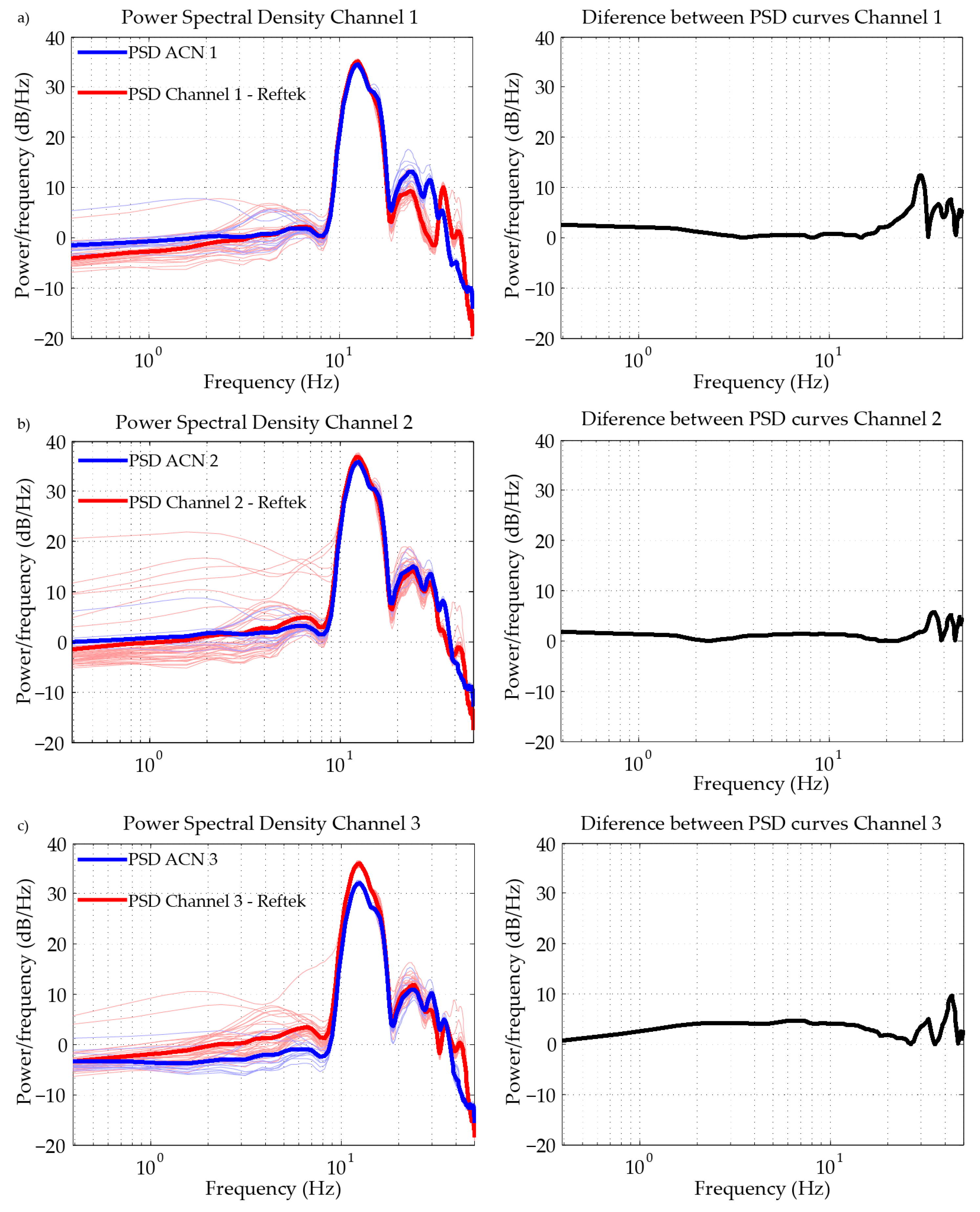
3.1. Frequency Response
3.2. Precision and Accuracy Tests
3.2.1. Precision
3.2.2. Accuracy
3.3. Synchronization Test
3.4. Battery Duration Test
4. Field Test for Validation
5. Conclusions
Supplementary Materials
Author Contributions
Funding
Acknowledgments
Conflicts of Interest
References
- Verma, M.; Singh, R.J.; Bansal, B.K. Soft sediments and damage pattern: A few case studies from large Indian earthquakes vis-a-vis seismic risk evaluation. Nat. Hazards 2014, 74, 1829–1851. [Google Scholar] [CrossRef]
- Panzera, F.; Rigano, R.; Lombardo, G.; Cara, F.; Di Giulio, G.; Rovelli, A. The role of alternating outcrops of sediments and basaltic lavas on seismic urban scenario: The study case of Catania, Italy. Bull. Earthq. Eng. 2010, 9, 411–439. [Google Scholar] [CrossRef]
- Firat, S.; Isik, N.S.; Arman, H.; Demir, M.; Vural, I. Investigation of the soil amplification factor in the Adapazari region. Bull. Eng. Geol. Environ. 2015, 75, 141–152. [Google Scholar] [CrossRef]
- Rost, S. Array seismology: Methods and applications. Rev. Geophys. 2002, 40, 1008. [Google Scholar] [CrossRef]
- Wang, N.; Zhang, N.; Wang, M. Wireless sensors in agriculture and food industry—Recent development and future perspective. Comput. Electron. Agric. 2006, 50, 1–14. [Google Scholar] [CrossRef]
- Ruiz-Garcia, L.; Barreiro, P.; Robla, J.I. Performance of ZigBee-Based wireless sensor nodes for real-time monitoring of fruit logistics. J. Food Eng. 2008, 87, 405–415. [Google Scholar] [CrossRef]
- Brunelli, D.; Rossi, M. Enhancing lifetime of WSN for natural gas leakages detection. Microelectron. J. 2014, 45, 1665–1670. [Google Scholar] [CrossRef]
- Khedo, K.K.; Perseedoss, R.; Mungur, A. A Wireless Sensor Network Air Pollution Monitoring System. Int. J. Wirel. Mob. Netw. 2010, 2, 31–45. [Google Scholar] [CrossRef]
- Jedermann, R.; Behrens, C.; Westphal, D.; Lang, W. Applying autonomous sensor systems in logistics—Combining sensor networks, RFIDs and software agents. Sens. Actuators A Phys. 2006, 132, 370–375. [Google Scholar] [CrossRef]
- Picozzi, M.; Milkereit, C.; Parolai, S.; Jaeckel, K.H.; Veit, I.; Fischer, J.; Zschau, J. GFZ wireless seismic array (GFZ-WISE), a wireless mesh network of seismic sensors: New perspectives for seismic noise array investigations and site monitoring. Sensors 2010, 10, 3280–3304. [Google Scholar] [CrossRef]
- Dai, K.; Li, X.; Lu, C.; You, Q.; Huang, Z.; Wu, H. A Low-Cost Energy-Efficient Cableless Geophone Unit for Passive Surface Wave Surveys. Sensors 2015, 15, 24698–24715. [Google Scholar] [CrossRef] [PubMed]
- Fischer, J.; Redlich, J.-P.; Zschau, J.; Milkereit, C.; Picozzi, M.; Fleming, K.; Brumbulli, M.; Lichtblau, B.; Eveslage, I. A wireless mesh sensing network for early warning. J. Netw. Comput. Appl. 2012, 35, 538–547. [Google Scholar] [CrossRef]
- Lopes Pereira, R.; Trindade, J.; Gonçalves, F.; Suresh, L.; Barbosa, D.; Vazão, T. A wireless sensor network for monitoring volcano-seismic signals. Nat. Hazards Earth Syst. Sci. 2014, 14, 3123–3142. [Google Scholar] [CrossRef]
- Peci, L.; Berrocoso, M.; Fernández-Ros, A.; García, A.; Marrero, J.; Ortiz, R. Embedded ARM System for Volcano Monitoring in Remote Areas: Application to the Active Volcano on Deception Island (Antarctica). Sensors 2014, 14, 672–690. [Google Scholar] [CrossRef] [PubMed]
- Texas Instruments. Available online: http://www.ti.com/lit/ds/sbas184d/sbas184d.pdf (accessed on 30 March 2019).
- Jamali-Rad, H.; Campman, X. Internet of Things-based wireless networking for seismic applications. Geophys. Prospect. 2018, 66, 833–853. [Google Scholar] [CrossRef]
- Martinez, K.; Hart, J.K.; Basford, P.J.; Bragg, G.M.; Ward, T.; Young, D.S. A geophone wireless sensor network for investigating glacier stick-slip motion. Comput. Geosci. 2017, 105, 103–112. [Google Scholar] [CrossRef]
- Boxberger, T.; Fleming, K.; Pittore, M.; Parolai, S.; Pilz, M.; Mikulla, S. The Multi-Parameter Wireless Sensing System (MPwise): Its Description and Application to Earthquake Risk Mitigation. Sensors 2017, 17, 2400. [Google Scholar] [CrossRef]
- Tian, R.; Wang, L.; Zhou, X.; Xu, H.; Lin, J.; Zhang, L.; Tian, R.; Wang, L.; Zhou, X.; Xu, H.; et al. An Integrated Energy-Efficient Wireless Sensor Node for the Microtremor Survey Method. Sensors 2019, 19, 544. [Google Scholar] [CrossRef]
- Dryden, M.D.M.; Fobel, R.; Fobel, C.; Wheeler, A.R. Upon the Shoulders of Giants: Open-Source Hardware and Software in Analytical Chemistry. Anal. Chem. 2017, 89, 4330–4338. [Google Scholar] [CrossRef]
- GitHub Where Open Source Communities Live. Available online: https://github.com/open-source (accessed on 3 October 2018).
- Delgado, J.; García-tortosa, F.J.; Garrido, J.; Giner, J.; Lenti, L. Engineering-geological model of the landslide of Güevejar (S Spain ) reactivated by historical earthquakes. In Proceedings of the EGU General Assembly 2015, Vienna, Austria, 12–17 April 2015. [Google Scholar]
- Soler-Llorens, J.L.; Galiana-Merino, J.J.; Giner-Caturla, J.J.; Jauregui-Eslava, P.; Rosa-Cintas, S.; Rosa-Herranz, J.; Nassim Benabdeloued, B.Y. Design and test of Geophonino-3D: A low-cost three-component seismic noise recorder for the application of the H/V method. Sens. Actuators A Phys. 2018, 269, 342–354. [Google Scholar] [CrossRef]
- Arduino Due and Mega + Shield Enclosure (Thingiverse). Available online: https://www.thingiverse.com/thing:1607720 (accessed on 16 April 2019).
- Baronti, P.; Pillai, P.; Chook, V.W.C.; Chessa, S.; Gotta, A.; Hu, Y.F. Wireless sensor networks: A survey on the state of the art and the 802.15.4 and ZigBee standards. Comput. Commun. 2007, 30, 1655–1695. [Google Scholar] [CrossRef]
- XBee ®/XBee-PRO ® RF Modules. Product Manual v1.xEx-802.15.4 Protocol. Available online: https://www.sparkfun.com/datasheets/Wireless/Zigbee/XBee-Datasheet.pdf (accessed on 14 August 2019).
- Xbee Arduino Library Used in Geophonino Development. Available online: hhttps://zenodo.org/record/2620960#.XYXxn6IRVPZ (accessed on 14 August 2019).
- TinyGPS: Mikal Hart TinyGPS Library Used in Geophonino Development. Available online: https://zenodo.org/record/2620984#.XYXxsqIRVPZ (accessed on 14 August 2019).
- Soler-Llorens, J.L.; Galiana-Merino, J.J.; Giner-Caturla, J.; Jauregui-Eslava, P.; Rosa-Cintas, S.; Rosa-Herranz, J. Development and programming of Geophonino: A low cost Arduino-based seismic recorder for vertical geophones. Comput. Geosci. 2016, 94, 1–10. [Google Scholar] [CrossRef]
- Bonnefoy-Claudet, S.; Cotton, F.; Bard, P.-Y. The nature of noise wavefield and its applications for site effects studies. Earth Sci. Rev. 2006, 79, 205–227. [Google Scholar] [CrossRef]
- Strollo, A.; Bindi, D.; Parolai, S.; Jäckel, K.-H. On the suitability of 1 s geophone for ambient noise measurements in the 0.1–20Hz frequency range: Experimental outcomes. Bull. Earthq. Eng. 2008, 6, 141–147. [Google Scholar] [CrossRef]
- Toksöz, M.N.; Lacoss, R.T. Microseisms: Mode structure and sources. Science 1968, 159, 872–873. [Google Scholar] [CrossRef] [PubMed]
- Lacoss, R.T.; Kelly, E.J.; Toksöz, M.N. Estimation of Seismic Noise Structure using Arrays. Geophysics 1969, 34, 21–38. [Google Scholar] [CrossRef]
- Park, C.B.; Miller, R.D. Multichannel Analysis of Passive Surface Waves—Modeling and Processing Schemes. In Site Characterization and Modeling; American Society of Civil Engineers: Reston, VA, USA, 2005; pp. 1–14. [Google Scholar]
- Louie, J.N. Faster, Better: Shear-Wave Velocity to 100 Meters Depth from Refraction Microtremor Arrays. Bull. Seismol. Soc. Am. 2001, 91, 347–364. [Google Scholar] [CrossRef]
- AKI, K. Space and time spectra of stationary stochastic waves, with spectral reference to microtremors. Bull. Earthq. Res. Inst. 1957, 35, 415–456. [Google Scholar]
- Okada, H.; Suto, K. The Microtremor Survey Method; Society of Exploration Geophysicists: Tulsa, OK, USA, 2003. [Google Scholar]
- Capon, J. High-resolution frequency-wavenumber spectrum analysis. Proc. IEEE 1969, 57, 1408–1418. [Google Scholar] [CrossRef]
- Rosa-Cintas, S.; Galiana-Merino, J.J.; Molina-Palacios, S.; Rosa-Herranz, J.; García-Fernández, M.; Jiménez, M.J. Soil characterization in urban areas of the Bajo Segura Basin (Southeast Spain) using H/V, F–K and ESAC methods. J. Appl. Geophys. 2011, 75, 543–557. [Google Scholar] [CrossRef]
- Stoffa, P.L.; Sen, M.K. Nonlinear multiparameter optimization using genetic algorithms: Inversion of plane-wave seismograms. Geophysics 1991, 56, 1794–1810. [Google Scholar] [CrossRef]
- Sambridge, M.; Drijkoningen, G. Genetic algorithms in seismic waveform inversion. Geophys. J. Int. 1992, 109, 323–342. [Google Scholar] [CrossRef]
- Lomax, A.; Snieder, R. Finding sets of acceptable solutions with a genetic algorithm with application to surface wave group dispersion in Europe. Geophys. Res. Lett. 1994, 21, 2617–2620. [Google Scholar] [CrossRef]
- Sambridge, M. Geophysical inversion with a neighbourhood algorithm-I. Searching a parameter space. Geophys. J. Int. 1999, 138, 479–494. [Google Scholar] [CrossRef]
- Wathelet, M. An improved neighborhood algorithm: Parameter conditions and dynamic scaling. Geophys. Res. Lett. 2008, 35, L09301. [Google Scholar] [CrossRef]
- Asten, M.W.; Henstridge, J.D. Array estimators and the use of microseisms for reconnaissance of sedimentary basins. Geophys. 1984, 49, 1828–1837. [Google Scholar] [CrossRef]
- Gil Perez, D. Modelización de la Microzonación Sísmica Mediante un Algoritmo de Interpolación de Máxima Vecindad. Final Project of Degree, University of Alicante, Alicante, Spain, September 2008. [Google Scholar]
- Rosa-Cintas, S.; Galiana-Merino, J.J.; Alfaro, P.; Rosa-Herranz, J. Optimizing the number of stations in arrays measurements: Experimental outcomes for different array geometries and the f–k method. J. Appl. Geophys. 2014, 102, 96–133. [Google Scholar] [CrossRef]
- Earth Data—PR6-24 Specification. Available online: http://www.earthdata.co.uk/pr6-24sp.html (accessed on 18 April 2019).
- SeistronixInc. Ras-24 Digital Seismograph Rev.1.04.3299D. 2005. Available online: http://www.seistronix.com/download/ras_ds_v105.pdf (accessed on 23 April 2019).
- Endrun, B.; Ohrnberger, M.; Savvaidis, A. On the repeatability and consistency of three-component ambient vibration array measurements. Bull. Earthq. Eng. 2010, 8, 535–570. [Google Scholar] [CrossRef]
- Rosa-Cintas, S.; Galiana-Merino, J.J.; Rosa-Herranz, J.; Molina, S.; Giner-Caturla, J. Suitability of 10 Hz vertical geophones for seismic noise array measurements based on frequency-wavenumber and extended spatial autocorrelation analyses. Geophys. Prospect. 2013, 61, 183–198. [Google Scholar] [CrossRef]
- Geopsy Software. Available online: http://www.geopsy.org/download.php (accessed on 18 April 2019).
- Wathelet, M. Array Recordings of Ambient Vibrations: Surface-Wave Inversion. Ph.D. Thesis, University of Liège, Liege, Belgium, February 2005. [Google Scholar]
- Mora Perez, I. Efectos de la Configuración en Array de Sensores en la Estimación de Perfiles de Velocidad Vs. Final Project of Degree, University of Alicante, Alicante, Spain, December 2008. [Google Scholar]


| Description | Value/Range |
|---|---|
| Operating Voltage | 5 V |
| Input Voltage (recommended) | 7–12 V |
| Input Voltage (limits) | 6–16 V |
| Digital I/O Pins | 54 (of which 12 provide PWM output) |
| Analog Input Pins | 12 |
| Analog Output Pins | 2 (DAC) |
| Total DC Output Current on al I/O lines | 130 mA |
| DC Current for 3.3 V and 5 V Pin | 800 mA |
| Flash Memory | 512 Kilobytes (KB) |
| SRAM | 96 KB (two banks: 64 KB and 32 KB) |
| Clock Speed | 84 MHz |
| Length | 101.52 mm |
| Width | 53.3 mm |
| Weight | 36 g. |
| Commercial equipment | Geophonino-W | |||
|---|---|---|---|---|
| Site | Kmax/2 | Kmin/2 | Kmax/2 | Kmin/2 |
| Almoradí | 0.470 | 0.027 | 0.319 | 0.056 |
| Rojales | 0.500 | 0.027 | 0.299 | 0.063 |
| Mutxamel | 0.065 | 0.031 | 0.255 | 0.046 |
| Catral | 0.533 | 0.096 | 0.319 | 0.056 |
© 2019 by the authors. Licensee MDPI, Basel, Switzerland. This article is an open access article distributed under the terms and conditions of the Creative Commons Attribution (CC BY) license (http://creativecommons.org/licenses/by/4.0/).
Share and Cite
Soler-Llorens, J.L.; Galiana-Merino, J.J.; Giner-Caturla, J.J.; Rosa-Cintas, S.; Nassim-Benabdeloued, B.Y. Geophonino-W: A Wireless Multichannel Seismic Noise Recorder System for Array Measurements. Sensors 2019, 19, 4087. https://doi.org/10.3390/s19194087
Soler-Llorens JL, Galiana-Merino JJ, Giner-Caturla JJ, Rosa-Cintas S, Nassim-Benabdeloued BY. Geophonino-W: A Wireless Multichannel Seismic Noise Recorder System for Array Measurements. Sensors. 2019; 19(19):4087. https://doi.org/10.3390/s19194087
Chicago/Turabian StyleSoler-Llorens, Juan Luis, Juan José Galiana-Merino, José Juan Giner-Caturla, Sergio Rosa-Cintas, and Boualem Youcef Nassim-Benabdeloued. 2019. "Geophonino-W: A Wireless Multichannel Seismic Noise Recorder System for Array Measurements" Sensors 19, no. 19: 4087. https://doi.org/10.3390/s19194087
APA StyleSoler-Llorens, J. L., Galiana-Merino, J. J., Giner-Caturla, J. J., Rosa-Cintas, S., & Nassim-Benabdeloued, B. Y. (2019). Geophonino-W: A Wireless Multichannel Seismic Noise Recorder System for Array Measurements. Sensors, 19(19), 4087. https://doi.org/10.3390/s19194087