Improving Accuracy of the Alpha–Beta Filter Algorithm Using an ANN-Based Learning Mechanism in Indoor Navigation System


Abstract
1. Introduction
2. Related Work
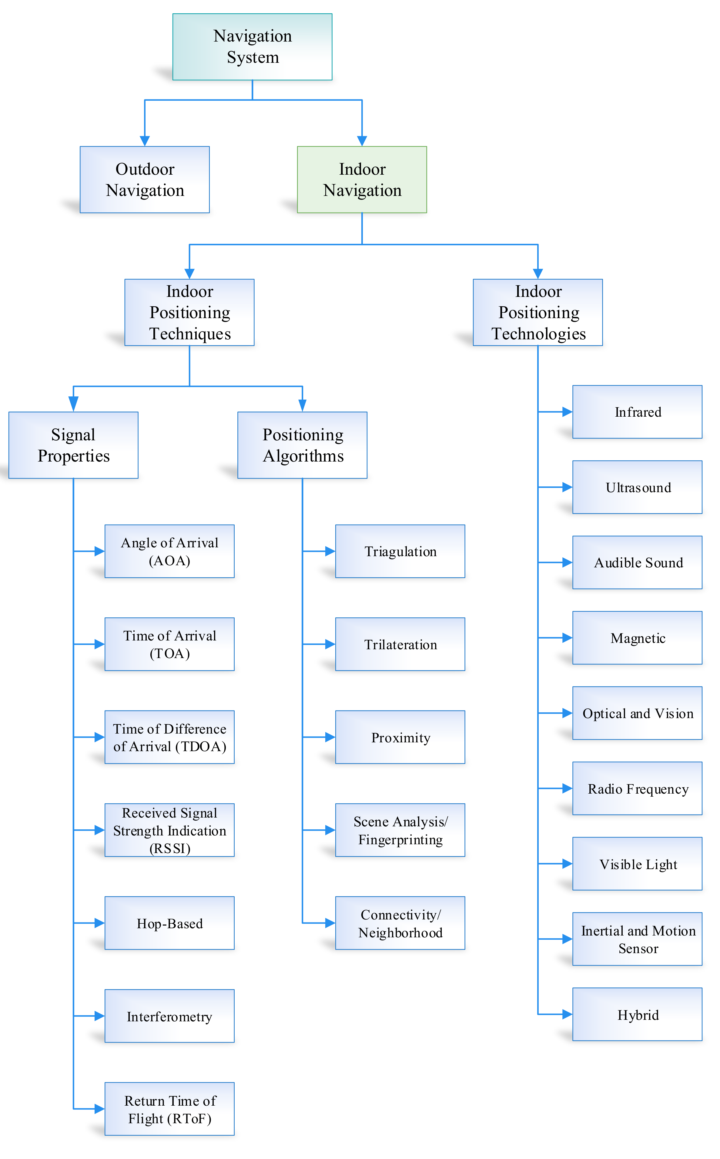
2.1. Inertial and Motion Sensor
2.1.1. Dead Reckonina
3. System Architecture of Proposed Indoor Navigation
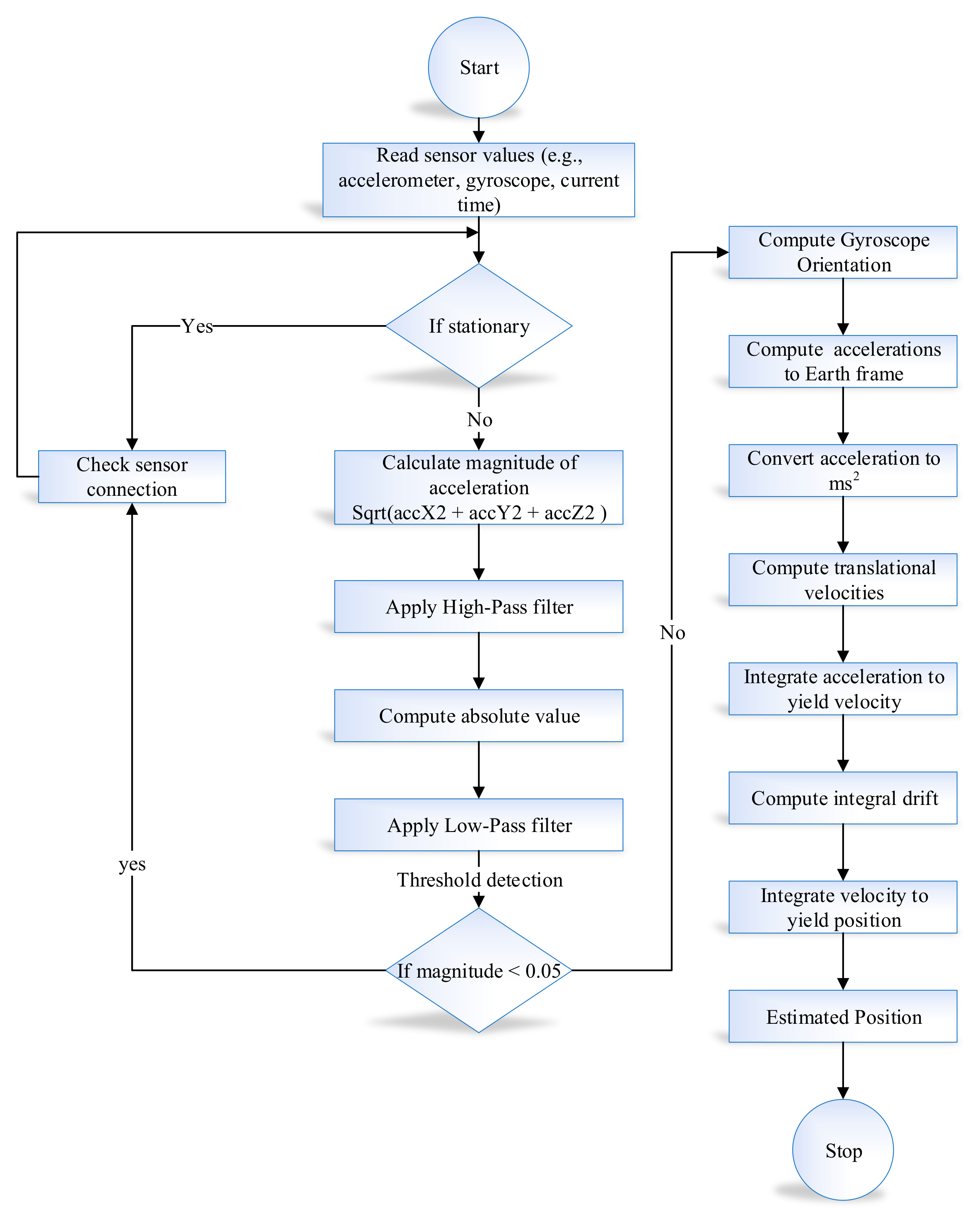
3.1. Scenario of Inertial Tracking in Indoor Navigation
3.1.1. Orientation Estimation from Gyroscope in Indoor Navigation
3.1.2. Orientation Estimation from Accelerometer in Indoor Navigation
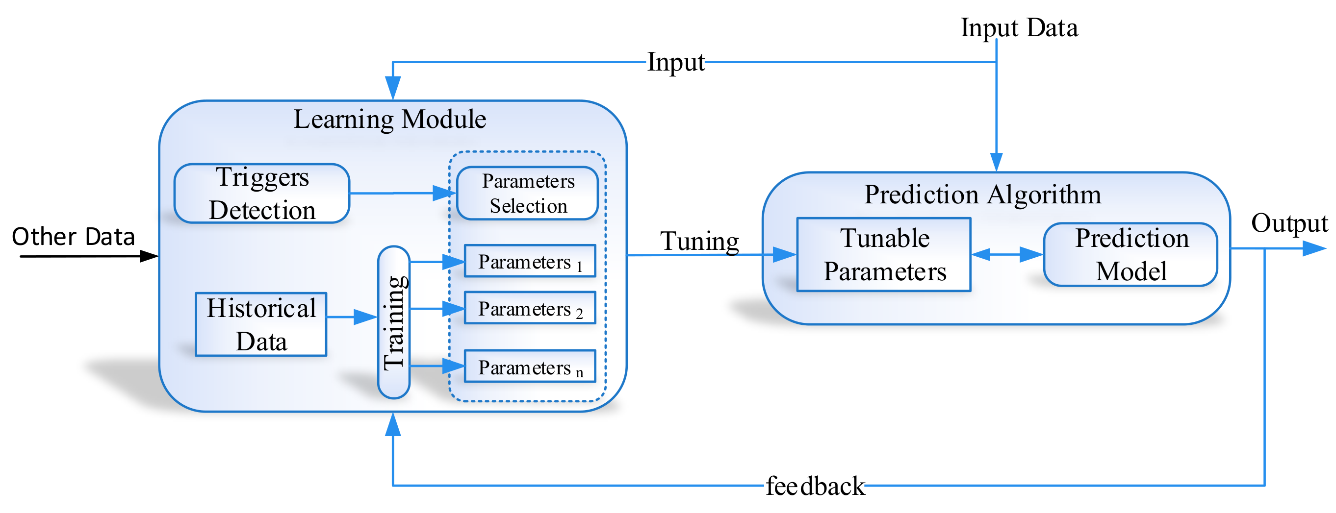
3.2. Proposed System Architecture of Learning to Prediction Scheme
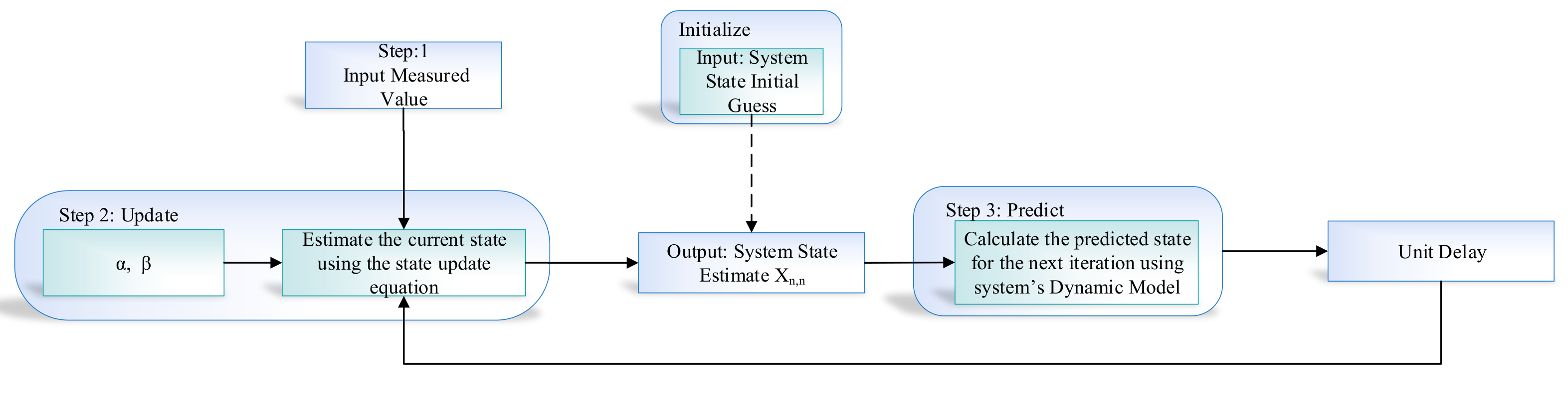
3.3. Alpha-Beta Filter Algorithm
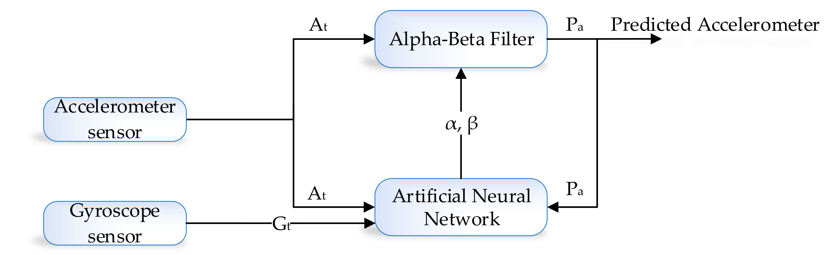
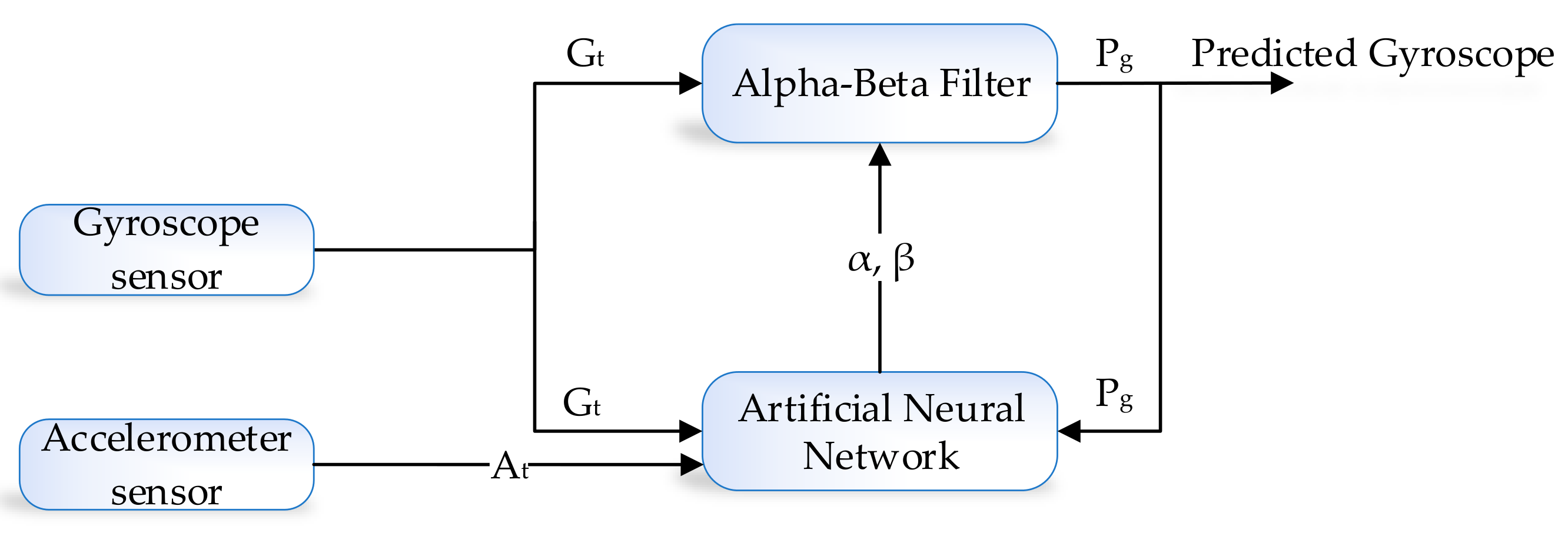
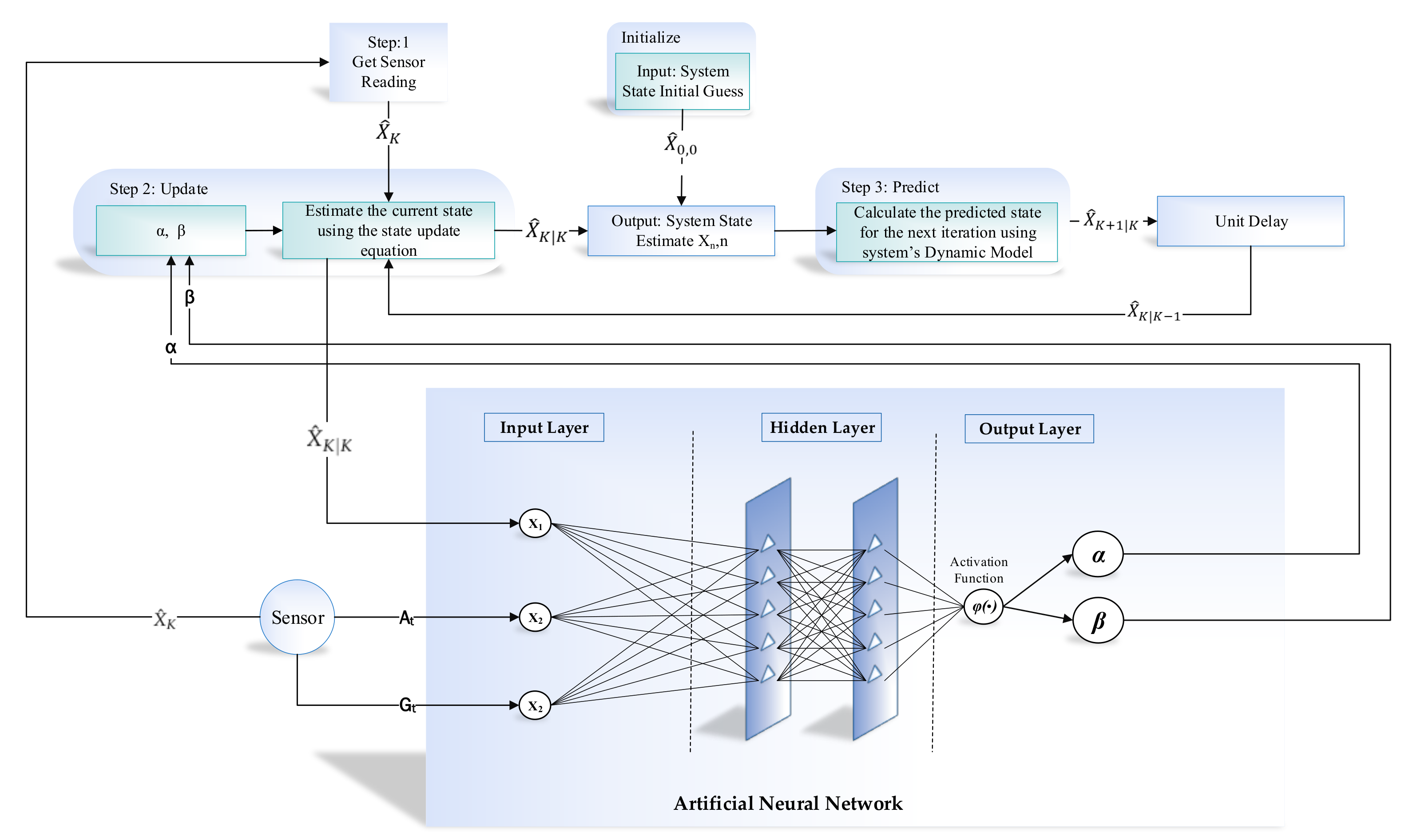
3.4. ANN-Based Learning to Prediction for the Alpha–Beta Filter
4. Implementation for ANN-Based Learning Mechanism in Indoor Navigation
4.1. Development Environment
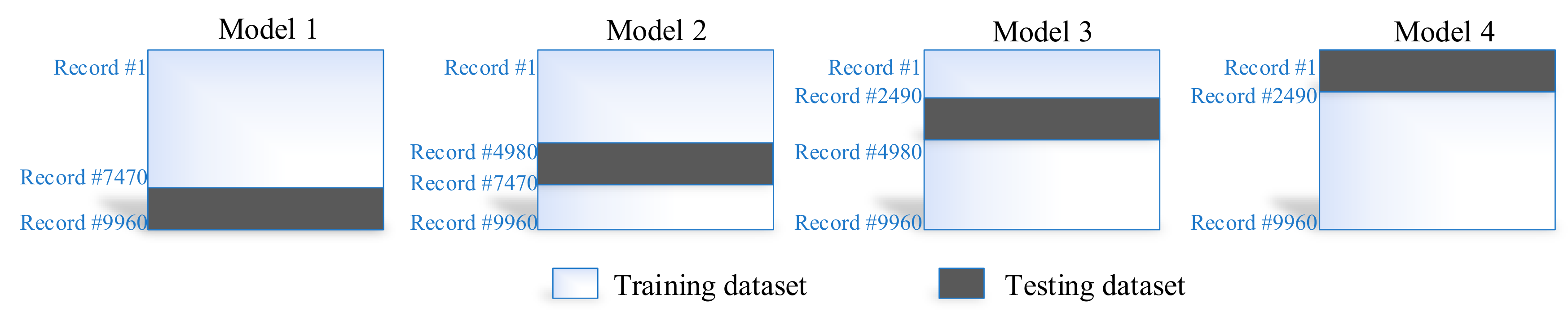
4.2. Implementation
5. Results and Discussions
6. Conclusions
Author Contributions
Funding
Acknowledgments
Conflicts of Interest
References
- Grewal, M.S.; Weill, L.R.; Andrews, A.P. Global Positioning Systems, Inertial Navigation, and Integration; John Wiley & Sons: Hoboken, NJ, USA, 2007. [Google Scholar]
- Koyuncu, H.; Yang, S.H. A survey of indoor positioning and object locating systems. IJCSNS Int. J. Comput. Sci. Netw. Secur. 2010, 10, 121–128. [Google Scholar]
- Fuchs, C.; Aschenbruck, N.; Martini, P.; Wieneke, M. Indoor tracking for mission critical scenarios: A survey. Pervasive Mob. Comput. 2011, 7, 1–15. [Google Scholar] [CrossRef]
- Rantakokko, J.; Händel, P.; Fredholm, M.; Marsten-Eklöf, F. User requirements for localization and tracking technology: A survey of mission-specific needs and constraints. In Proceedings of the International Conference on Indoor Positioning and Indoor Navigation (IPIN 2010), Zurich, Switzerland, 15–17 September 2010; pp. 1–9. [Google Scholar]
- Khudhair, A.A.; Jabbar, S.Q.; Sulttan, M.Q.; Wang, D. Wireless indoor localization systems and techniques: survey and comparative study. Indones. J. Electr. Eng. Comput. Sci. 2016, 3, 392–409. [Google Scholar] [CrossRef]
- Brena, R.F.; García-Vázquez, J.P.; Galván-Tejada, C.E.; Muñoz-Rodriguez, D.; Vargas-Rosales, C.; Fangmeyer, J. Evolution of indoor positioning technologies: A survey. J. Sens. 2017, 2017, 2630413. [Google Scholar] [CrossRef]
- Gu, Y.; Lo, A.; Niemegeers, I. A survey of indoor positioning systems for wireless personal networks. IEEE Commun. Surv. Tutor. 2009, 11, 13–32. [Google Scholar] [CrossRef]
- Kok, M.; Hol, J.D.; Schön, T.B. Using inertial sensors for position and orientation estimation. arXiv 2017, arXiv:1704.06053. [Google Scholar] [CrossRef]
- Faramondi, L.; Inderst, F.; Pascucci, F.; Setola, R.; Delprato, U. An enhanced indoor positioning system for first responders. In Proceedings of the 4th International Conference on Indoor Positioning and Indoor Navigation (IPIN 2013), Montbeliard-Belfort, France, 28–31 October 2013; pp. 1–8. [Google Scholar]
- Filippeschi, A.; Schmitz, N.; Miezal, M.; Bleser, G.; Ruffaldi, E.; Stricker, D. Survey of motion tracking methods based on inertial sensors: A focus on upper limb human motion. Sensors 2017, 17, 1257. [Google Scholar] [CrossRef]
- Arraigada, M.; Partl, M. Calculation of displacements of measured accelerations, analysis of two accelerometers and application in road engineering. In Proceedings of the 6th Swiss Transport Research Conference (STRC 2006), Monte Verità, Ascona, Switzerland, 15–17 March 2006; p. 30. [Google Scholar]
- Seifert, K.; Camacho, O. Implementing positioning algorithms using accelerometers. Free. Semicond. 2007, 1–13. [Google Scholar]
- Abellanosa, C.B.; Lugpatan, R.P.J.; Pascua, D.A.D. Position estimation using inertial measurement unit (IMU) on a quadcopter in an enclosed environment. Int. J. Comput. Commun. Instrum. Eng. 2016, 3, 332–336. [Google Scholar]
- Pastell, M.; Frondelius, L.; Järvinen, M.; Backman, J. Filtering methods to improve the accuracy of indoor positioning data for dairy cows. Biosyst. Eng. 2018, 169, 22–31. [Google Scholar] [CrossRef]
- Bozkurt, S.; Elibol, G.; Gunal, S.; Yayan, U. A comparative study on machine learning algorithms for indoor positioning. In Proceedings of the 2015 International Symposium on Innovations in Intelligent SysTems and Applications (INISTA), Madrid, Spain, 2–4 September 2015; pp. 1–8. [Google Scholar]
- Muset, B.; Emerich, S. Distance measuring using accelerometer and gyroscope sensors. Carpathian J. Electron. Comput. Eng. 2012, 5, 83. [Google Scholar]
- Feliz Alonso, R.; Zalama Casanova, E.; Gómez García-Bermejo, J. Pedestrian tracking using inertial sensors. J. Phys. Agents 2009, 3, 35–43. [Google Scholar] [CrossRef]
- Zhou, H.; Stone, T.; Hu, H.; Harris, N. Use of multiple wearable inertial sensors in upper limb motion tracking. Med. Eng. Phys. 2008, 30, 123–133. [Google Scholar] [CrossRef]
- El-Gohary, M.; McNames, J. Shoulder and elbow joint angle tracking with inertial sensors. IEEE Trans. Biomed. Eng. 2012, 59, 2635–2641. [Google Scholar] [CrossRef] [PubMed]
- Lang, P.; Kusej, A.; Pinz, A.; Brasseur, G. Inertial tracking for mobile augmented reality. In Proceedings of the 19th IEEE Instrumentation and Measurement Technology Conference, Anchorage, AK, USA, 21–23 May 2002; pp. 1583–1587. [Google Scholar]
- Dong, Y.; Scisco, J.; Wilson, M.; Muth, E.; Hoover, A. Detecting periods of eating during free-living by tracking wrist motion. IEEE J. Biomed. Health Inform. 2013, 18, 1253–1260. [Google Scholar] [CrossRef] [PubMed]
- Luzum, B. Navigation Principles of Positioning and Guidance. Eos Trans. Am. Geophys. Union 2004, 85, 110. [Google Scholar] [CrossRef]
- Harle, R. A survey of indoor inertial positioning systems for pedestrians. IEEE Commun. Surv. Tutor. 2013, 15, 1281–1293. [Google Scholar] [CrossRef]
- Sharp, I.; Yu, K. Sensor-based dead-reckoning for indoor positioning. Phys. Commun. 2014, 13, 4–16. [Google Scholar] [CrossRef]
- Diaz, E.M.; Gonzalez, A.L.M.; de Ponte Müller, F. Standalone inertial pocket navigation system. In Proceedings of the IEEE/ION Position, Location and Navigation Symposium (PLANS 2014), Monterey, CA, USA, 5–8 May 2014; pp. 241–251. [Google Scholar]
- Godha, S.; Cannon, M. GPS/MEMS INS integrated system for navigation in urban areas. Gps Solut. 2007, 11, 193–203. [Google Scholar] [CrossRef]
- Zhang, H.; Yuan, W.; Shen, Q.; Li, T.; Chang, H. A handheld inertial pedestrian navigation system with accurate step modes and device poses recognition. IEEE Sens. J. 2014, 15, 1421–1429. [Google Scholar] [CrossRef]
- Bird, J.; Arden, D. Indoor navigation with foot-mounted strapdown inertial navigation and magnetic sensors [emerging opportunities for localization and tracking]. IEEE Wirel. Commun. 2011, 18, 28–35. [Google Scholar] [CrossRef]
- Goyal, P.; Ribeiro, V.J.; Saran, H.; Kumar, A. Strap-down pedestrian dead-reckoning system. In Proceedings of the International Conference on Indoor Positioning and Indoor Navigation (IPIN 2011), Guimaraes, Portugal, 21–23 September 2011; pp. 1–7. [Google Scholar]
- Gusenbauer, D.; Isert, C.; Krösche, J. Self-contained indoor positioning on off-the-shelf mobile devices. In Proceedings of the International Conference on Indoor Positioning and Indoor Navigation (IPIN 2010), Zurich, Switzerland, 15–17 September 2010; pp. 1–9. [Google Scholar]
- Li, B.; Gallagher, T.; Dempster, A.G.; Rizos, C. How feasible is the use of magnetic field alone for indoor positioning? In Proceedings of the International Conference on Indoor Positioning and Indoor Navigation (IPIN 2012), Sydney, NSW, Australia, 13–15 November 2012; pp. 1–9. [Google Scholar]
- Liu, Z.; Zhang, L.; Liu, Q.; Yin, Y.; Cheng, L.; Zimmermann, R. Fusion of magnetic and visual sensors for indoor localization: Infrastructure-free and more effective. IEEE Trans. Multimed. 2016, 19, 874–888. [Google Scholar] [CrossRef]
- Penoyer, R. The alpha–beta filter. C User J. 1993, 11, 73–86. [Google Scholar]
- Next Generation Inertial Measurement Unit x-io Technologies Limited. Available online: https://x-io.co.uk/ngimu/ (accessed on 20 August 2019).


| Signal | Property | Measurement | Metric |
|---|---|---|---|
| Angle of Arrival (AOA) | Angle-based | High accuracy at room level | Complex, expensive and low accuracy at wide coverage |
| Received Signal Strength Indication (RSSI) | Signal-based (RSS) | Medium accuracy | Low cost |
| Time of Arrival (TOA) | Distance-based | High accuracy | Complex and expensive |
| Time Difference of Arrival (TDOA) | Distance-based | High accuracy | Expensive |
| Hop-Based | Signal-based | High accuracy | Complex and expensive with short range coverage |
| Interferometry | Signal-based | Medium accuracy | Complex with low accuracy |
| Return Time of Flight (RToF) | Signal-based | Low accuracy | Short range coverage |
| Positioning Algorithm | Signal Property | Pros | Cons |
|---|---|---|---|
| Triangulation | AOA | High accuracy at room level | Complex, expensive and low accuracy at wide coverage |
| Trilateration | TOA/TDOA | Medium accuracy | Complex and expensive |
| Proximity | RSSI | High accuracy | Complex and expensive |
| Connectivity/ Neighbourhood | RSSI/ Hop-based | High accuracy | Complex, expensive, short coverage |
| Scene analysis/fingerprinting | RSSI | High performance | Complex, expensive, medium accuracy and time consuming |
| Technology | Technique | Algorithm | Accuracy | Cost | Complexity | Scalability | Real-time |
|---|---|---|---|---|---|---|---|
| Infrared | Trilateration | TOA, TDOA | Medium | Low | High | Medium | Yes |
| Audible sound | Trilateration | TOA | Medium | Medium | Medium | Medium | Yes |
| Magnetic | Triangulation | AOA, TOA | High | High | High | Low | Yes |
| Bluetooth | Trilateration, fingerprinting | TDOA, RSSI | Low | Medium | Medium | Medium | Yes |
| WLAN | Trilateration, fingerprinting | TDOA, RSSI | Low | Medium | High | Medium | Yes |
| RFID | Fingerprinting | RSSI | Low | Medium | Medium | High | Yes |
| UWB | Trilateration | TOA, TDOA | High | Medium | Medium | Medium | Yes |
| NFC | Proximity | RSSI | High | Low | Low | High | No |
| WSN | Fingerprinting | RSSI | Medium | Medium | Medium | Medium | Yes |
| PDR/INS | DR | EKF, PF | Medium | Low | Low | Medium | Yes |
| Sensor | Description | |
|---|---|---|
| Gyroscope | Range | ±/s |
| Resolution | /s | |
| Sample Rate | 400 Hz | |
| Accelerometer | Range | ±16 g |
| Resolution | g | |
| Sample Rate | 400 Hz | |
| Magnetometer | Range | ±T |
| Resolution | ∼0.3 T | |
| Sample Rate | ∼20 Hz | |
| Component | Description |
|---|---|
| IDE | MATLAB R2018a |
| Operating System | Window 10 |
| CPU | Intel(R) Core(TM) i5-8500 CPU@3.00GHz |
| Memory | 8GB |
| Signal Processing Filter | Butterworth Digital Filter |
| Data Smoothing Algorithm | Alpha-Beta filter |
| Component | Description |
|---|---|
| IDE | MATLAB R2018a |
| Operating System | Window 10 |
| CPU | Intel(R) Core(TM) i5-8500 CPU@3.00GHz |
| Memory | 8GB |
| Artificial Neural Network | Feed Forward Backpropagation |
| Neuron in Hidden Layer | 10 |
| Neuron in output Layer | 2 |
| Number of Input | 3 |
| Prediction Algorithm | Alpha-Beta filter |
| Experiment ID | ANN Configuration | Model 1 | Model 2 | Model 3 | Model 4 | Model Average (Test Cases) | Experiments Average (Test Case) | ||||||
|---|---|---|---|---|---|---|---|---|---|---|---|---|---|
| Activation Function | Hidden Layers | Learning Rate | Trainina | Test | Trainina | Test | Trainina | Test | Trainina | Test | |||
| 1 | Sigmoid | 10 | 0.1 | 0.25 | 0.22 | 0.12 | 0.12 | 0.25 | 0.25 | 0.21 | 0.24 | 0.20 | 0.23 |
| 2 | Sigmoid | 10 | 0.1 | 0.26 | 0.23 | 0.25 | 0.26 | 0.28 | 0.28 | 0.50 | 0.35 | 0.28 | |
| 3 | Sigmoid | 10 | 0.1 | 0.29 | 0.24 | 0.15 | 0.17 | 0.10 | 0.12 | 0.32 | 0.35 | 0.22 | |
| 1 | Linear | 10 | 0.1 | 4.56 | 5.22 | 5.06 | 3.20 | 4.48 | 5.07 | 4.58 | 4.90 | 4.59 | 4.59 |
| 2 | Linear | 10 | 0.1 | 4.56 | 5.22 | 5.06 | 3.20 | 4.48 | 5.07 | 4.58 | 4.90 | 4.59 | |
| 3 | Linear | 10 | 0.1 | 4.56 | 5.22 | 5.06 | 3.20 | 4.48 | 5.07 | 4.58 | 4.90 | 4.59 | |
| 1 | Sigmoid | 10 | 0.2 | 0.19 | 0.15 | 0.08 | 0.09 | 0.20 | 0.22 | 0.24 | 0.27 | 0.18 | 0.19 |
| 2 | Sigmoid | 10 | 0.2 | 0.24 | 0.25 | 0.18 | 0.20 | 0.19 | 0.20 | 0.18 | 0.19 | 0.21 | |
| 3 | Sigmoid | 10 | 0.2 | 0.24 | 0.19 | 0.15 | 0.16 | 0.24 | 0.24 | 0.22 | 0.23 | 0.20 | |
| 1 | Linear | 10 | 0.2 | 4.44 | 5.18 | 5.03 | 3.17 | 4.49 | 5.04 | 4.55 | 4.87 | 4.56 | 4.56 |
| 2 | Linear | 10 | 0.2 | 4.44 | 5.18 | 5.03 | 3.17 | 4.49 | 5.04 | 4.55 | 4.87 | 4.56 | |
| 3 | Linear | 10 | 0.2 | 4.44 | 5.18 | 5.03 | 3.17 | 4.49 | 5.04 | 4.55 | 4.87 | 4.56 | |
| 1 | Sigmoid | 15 | 0.1 | 1.15 | 0.91 | 0.27 | 0.34 | 0.34 | 0.33 | 0.24 | 0.27 | 0.46 | 0.33 |
| 2 | Sigmoid | 15 | 0.1 | 0.13 | 0.11 | 0.23 | 0.25 | 0.23 | 0.20 | 0.31 | 0.31 | 0.21 | |
| 3 | Sigmoid | 15 | 0.1 | 0.57 | 0.45 | 0.34 | 0.36 | 0.22 | 0.22 | 0.19 | 0.23 | 0.31 | |
| 1 | Linear | 15 | 0.1 | 4.45 | 5.19 | 5.04 | 3.18 | 4.50 | 5.05 | 4.56 | 4.88 | 4.57 | 4.57 |
| 2 | Linear | 15 | 0.1 | 4.45 | 5.19 | 5.04 | 3.18 | 4.50 | 5.05 | 4.56 | 4.88 | 4.57 | |
| 3 | Linear | 15 | 0.1 | 4.45 | 5.19 | 5.04 | 3.18 | 4.50 | 5.05 | 4.56 | 4.88 | 4.57 | |
| 1 | Sigmoid | 15 | 0.2 | 0.27 | 0.23 | 0.56 | 0.91 | 0.19 | 0.22 | 0.40 | 0.40 | 0.44 | 0.30 |
| 2 | Sigmoid | 15 | 0.2 | 0.24 | 0.20 | 0.22 | 0.25 | 0.26 | 0.29 | 0.20 | 0.23 | 0.24 | |
| 3 | Sigmoid | 15 | 0.2 | 0.25 | 0.19 | 0.20 | 0.24 | 0.21 | 0.22 | 0.21 | 0.24 | 0.22 | |
| 1 | Linear | 15 | 0.2 | 4.45 | 5.19 | 5.04 | 3.18 | 4.50 | 5.05 | 4.56 | 4.88 | 4.57 | 4.57 |
| 2 | Linear | 15 | 0.2 | 4.45 | 5.19 | 5.04 | 3.18 | 4.50 | 5.05 | 4.56 | 4.88 | 4.57 | |
| 3 | Linear | 15 | 0.2 | 4.45 | 5.19 | 5.04 | 3.18 | 4.50 | 5.05 | 4.56 | 4.88 | 4.57 | |
| Experiment ID | Position Error | Position Error with Proposed Learning to Prediction Model |
|---|---|---|
| 1 | 0.130 mm | 0.102 mm |
| 2 | 0.115 mm | 0.098 mm |
| 3 | 0.135 mm | 0.112 mm |
| Metric | Alpha-Beta Filter | Alpha-Beta with Learning Module | ||
|---|---|---|---|---|
| R = 0.02 | R = 0.1 | |||
| RMSE | 2.494 | 2.527 | 2.388 | 2.481 |
| MAD | 0.163 | 0.166 | 0.156 | 0.165 |
| MSE | 6.222 | 6.388 | 5.701 | 6.155 |
| MAE | 0.997 | 1.137 | 0.931 | 1.2156 |
© 2019 by the authors. Licensee MDPI, Basel, Switzerland. This article is an open access article distributed under the terms and conditions of the Creative Commons Attribution (CC BY) license (http://creativecommons.org/licenses/by/4.0/).
Share and Cite
Jamil, F.; Kim, D.H. Improving Accuracy of the Alpha–Beta Filter Algorithm Using an ANN-Based Learning Mechanism in Indoor Navigation System. Sensors 2019, 19, 3946. https://doi.org/10.3390/s19183946
Jamil F, Kim DH. Improving Accuracy of the Alpha–Beta Filter Algorithm Using an ANN-Based Learning Mechanism in Indoor Navigation System. Sensors. 2019; 19(18):3946. https://doi.org/10.3390/s19183946
Chicago/Turabian StyleJamil, Faisal, and Do Hyeun Kim. 2019. "Improving Accuracy of the Alpha–Beta Filter Algorithm Using an ANN-Based Learning Mechanism in Indoor Navigation System" Sensors 19, no. 18: 3946. https://doi.org/10.3390/s19183946
APA StyleJamil, F., & Kim, D. H. (2019). Improving Accuracy of the Alpha–Beta Filter Algorithm Using an ANN-Based Learning Mechanism in Indoor Navigation System. Sensors, 19(18), 3946. https://doi.org/10.3390/s19183946