Marine Observation Beacon Clustering and Recycling Technology Based on Wireless Sensor Networks


Abstract
1. Introduction
- ♦
- We divide the recycling process of the marine observation beacon into three phases. The algorithm is designed to meet the demands of different phases.
- ♦
- A novel scheme is proposed where the FLS is used to comprehensively consider the influence of various environmental factors on the path weight, breaking through the limitations of traditional description methods.
- ♦
- We propose an effective solution by using centralized and distributed algorithms. After the BS completes the clustering, the CH replacement is completed by the nodes in the cluster. Nodes reduce unnecessary communication energy consumption, which extends the network life cycle.
2. Network Model
2.1. Node Model
- (1)
- This paper assumes that nodes are distributed over a continuous two-dimensional plane. This plane has no isolated points (beyond the communication range of all other nodes).
- (2)
- The node uses the LoRa (Long Range Radio) module to communicate, and the nodes in different clusters can be simultaneously communicated by changing the LoRa frequency band.
- (3)
- Node information: n nodes are randomly and independently distributed in a circular area. The size of the area is , where R is the radius. Node information is represented by , and the initial energy of the node is , where . Due to the difference between the beacon battery and the beacon start-up time, the initial power of each node is different.
- (4)
- The node controls the node communication range by controlling the transmission power.
- (5)
- All nodes are positioned and calibrated periodically by a global positioning system (GPS).
- (6)
- Each node has a unique identifier (ID) number and has small computing and storage capacity.
- (7)
- It is assumed that the CH receives k bits of data from each node and can be compressed into k bits of data.
2.2. Energy Model
2.3. Node Movement Model
- (1)
- Random walk;
- (2)
- Random waypoint mobile model;
- (3)
- Random direction model;
- (4)
- Gauss Markov model.
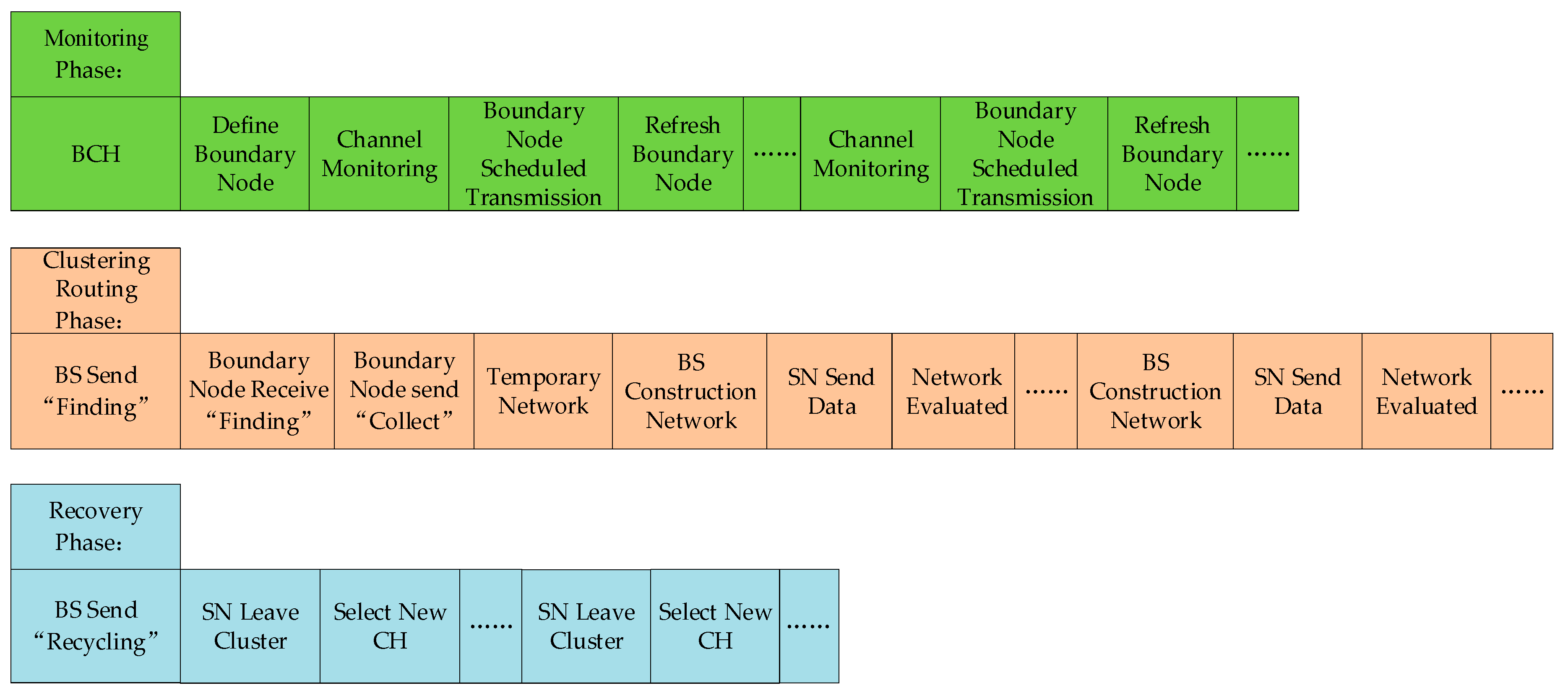
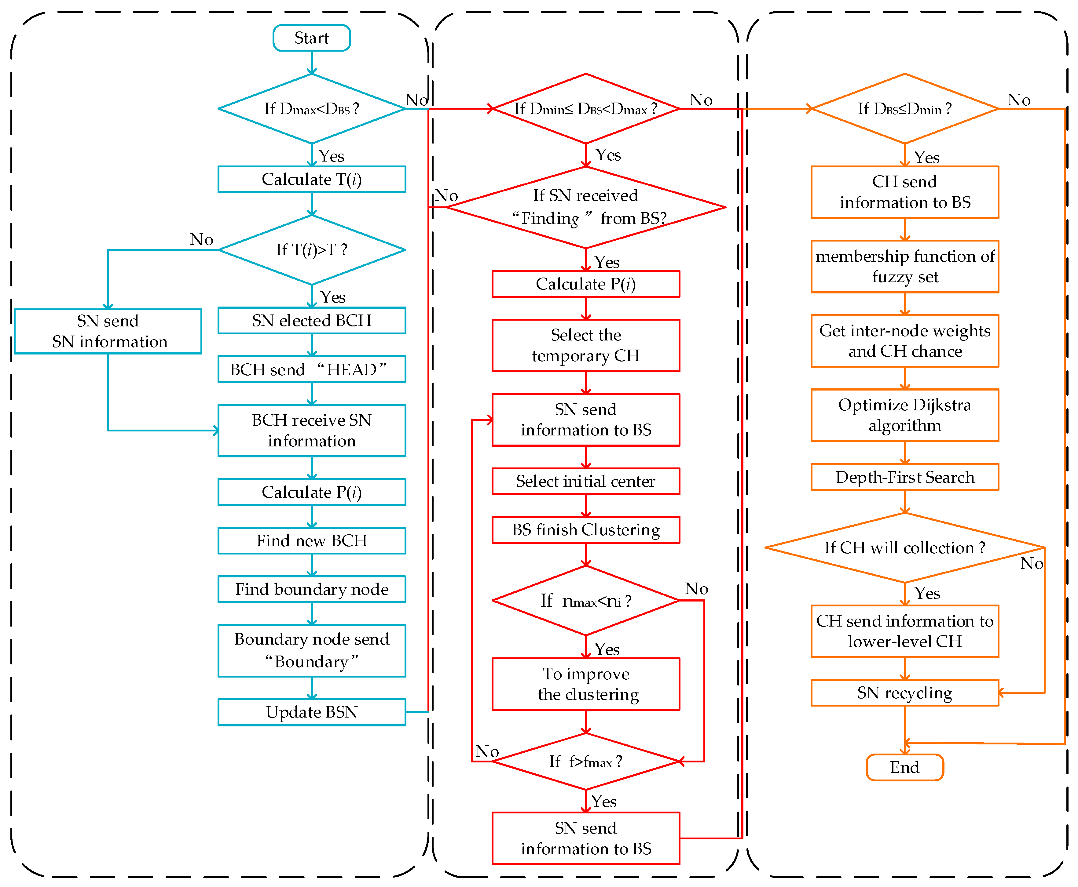
3. Proposed KFNS Algorithm
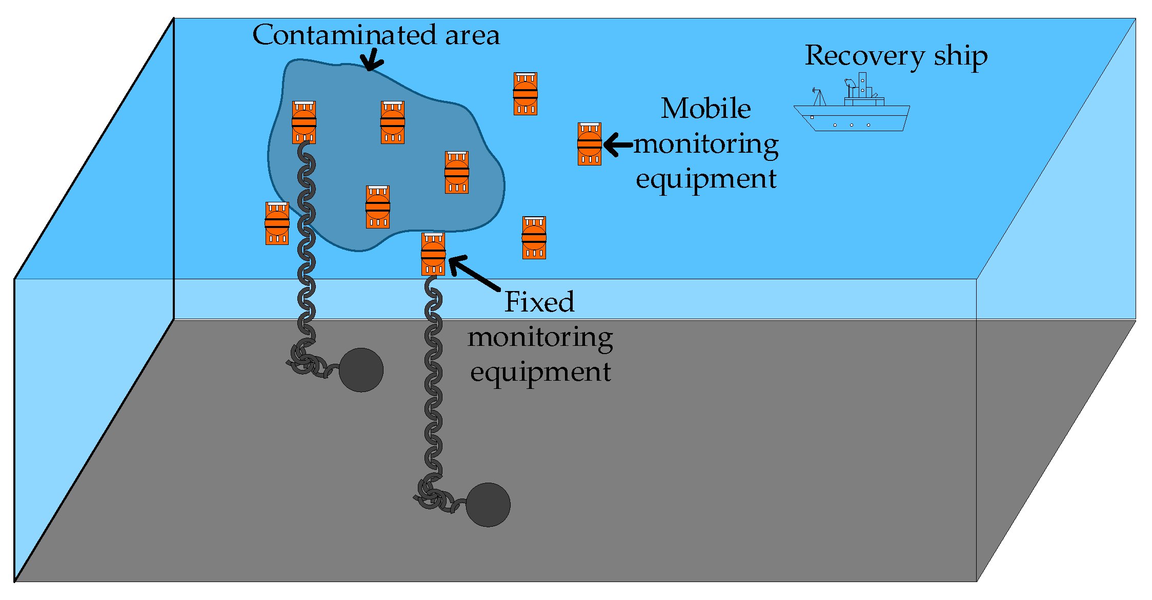
3.1. Monitoring Phase
3.2. Cluster Routing Phase
3.2.1. Temporary Network Routing
3.2.2. Enhanced K-Means Algorithm
| Algorithm 1 Improved k-means algorithm |
| Input: , , //set of ordinary sensor nodes and |
| j boundary sensor nodes. |
| Output: A set of k clusters |
| 1: for to do |
| 2: |
| 3: choose centroid among belong to |
| 4: for each set do |
| 5: assign to the cluster with nearest i.e. |
| 6: end for |
| 7: repeat |
| 8: for all and cluster do |
| 9: the centroid to be the center of all nodes in , so that |
| 10: end for |
| 11: until <V (i.e. less than the threshold) |
| 12: calculate criterion function |
| 13: end for |
| 14: find the minimum of E and get the optimal |
| 15: determine the optimal |
| 16: return |
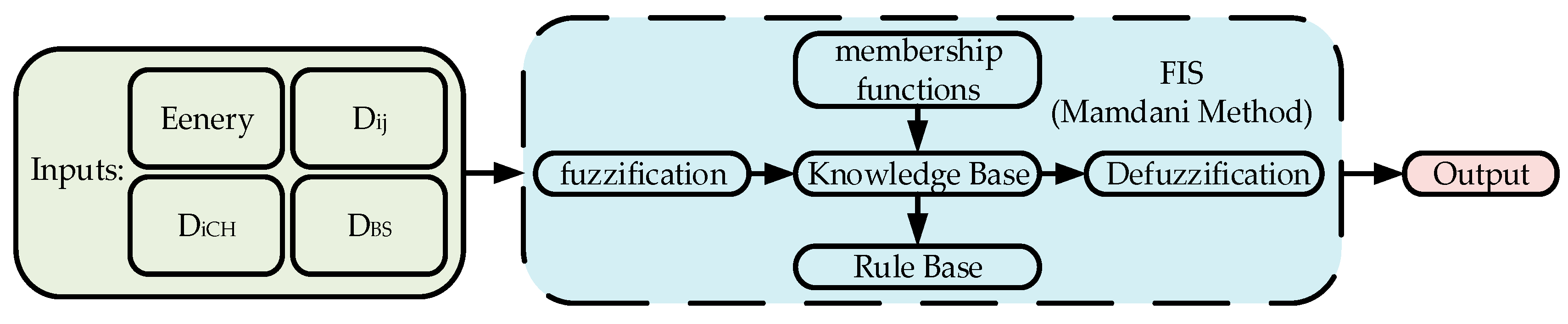
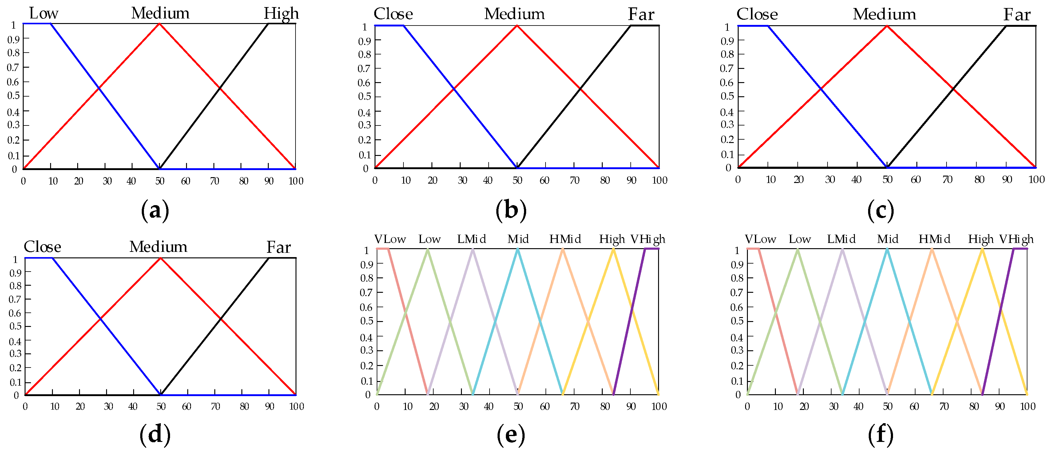
3.3. Recovery Phase
| Algorithm 2 Compute node recovery order |
| Input: , , , |
| Output: node recycling order |
| 1: Min–max normalization technique: |
| 2: add membership function of fuzzy set |
| 3: get inter-node weights and CH chance |
| 4: initialize , |
| 5: for do |
| 6: if && |
| 7: |
| 8: |
| 9: end if |
| 10: end for |
| 11: for do// Relaxed edge |
| 12: if && > + |
| 13: = + |
| 14: end if |
| 15: end for |
| 16: get the node to BS minimum weight path |
| 17: DFS { |
| 18: judging the boundary |
| 19: for do |
| 20: DFS (step+1) |
| 21: end for |
| 22: return} |
4. Simulation and Experiments
4.1. Monitoring Phase Simulation
4.1.1. Single-Hop Coverage Simulation
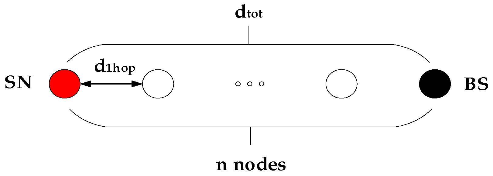
4.1.2. Multi-Hop Coverage Simulation
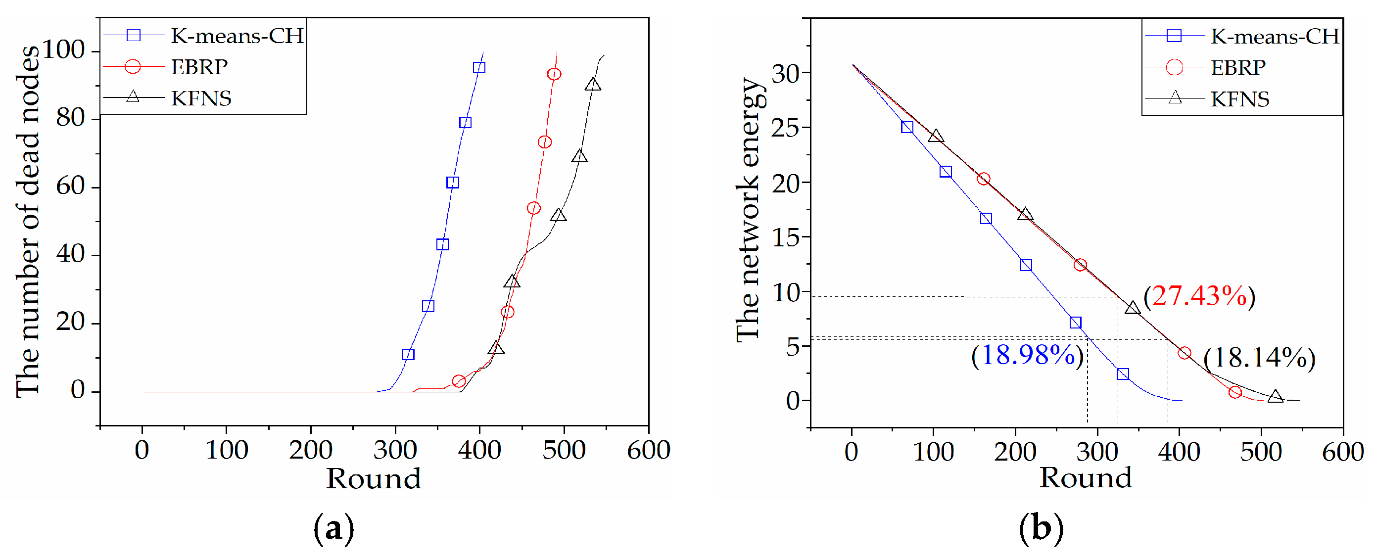
4.2. Cluster Routing Phase Simulation
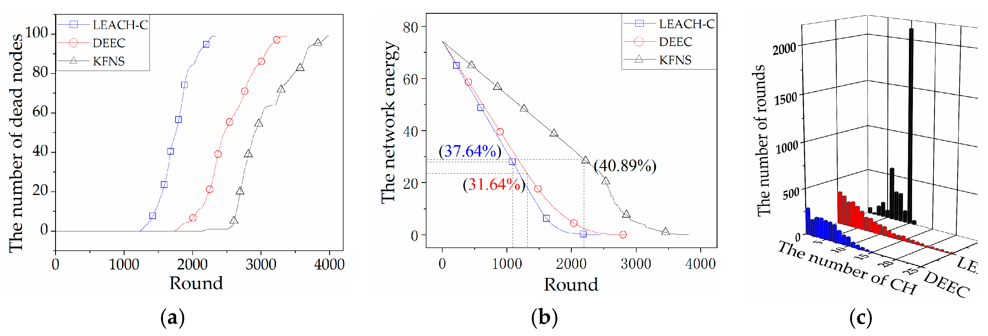
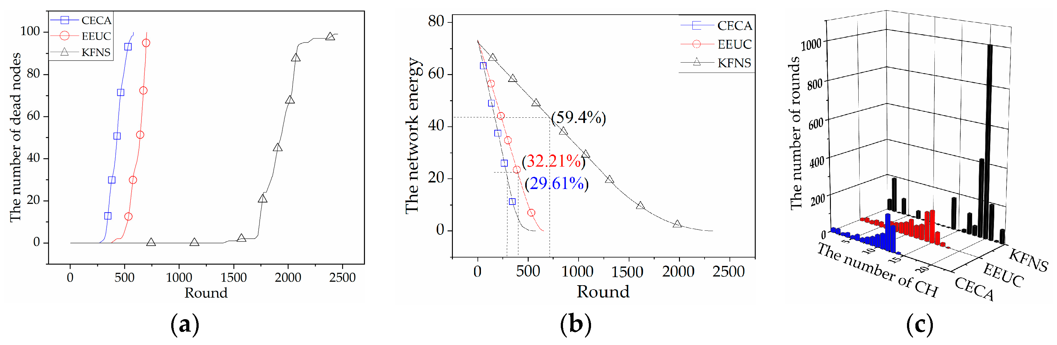
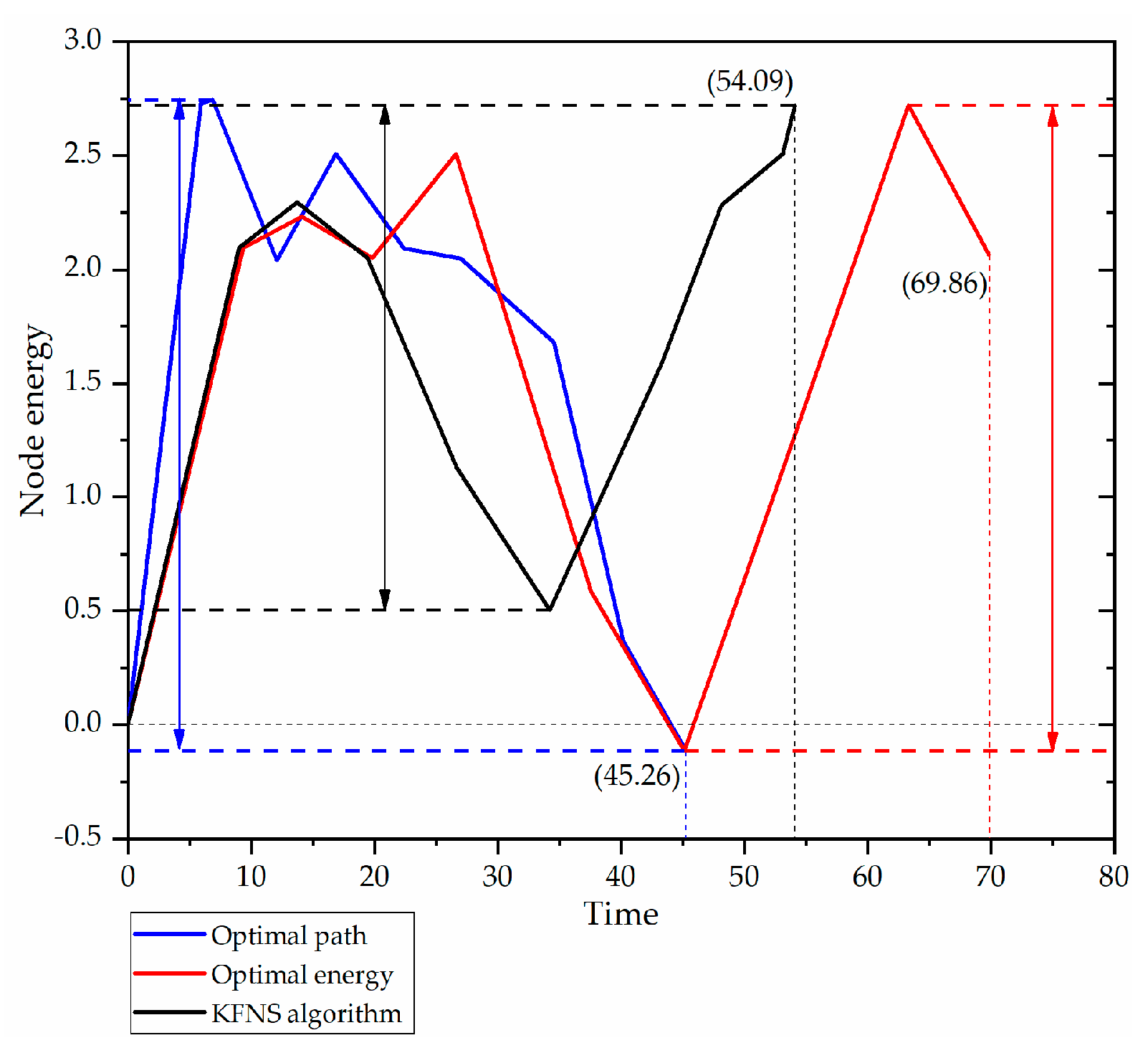
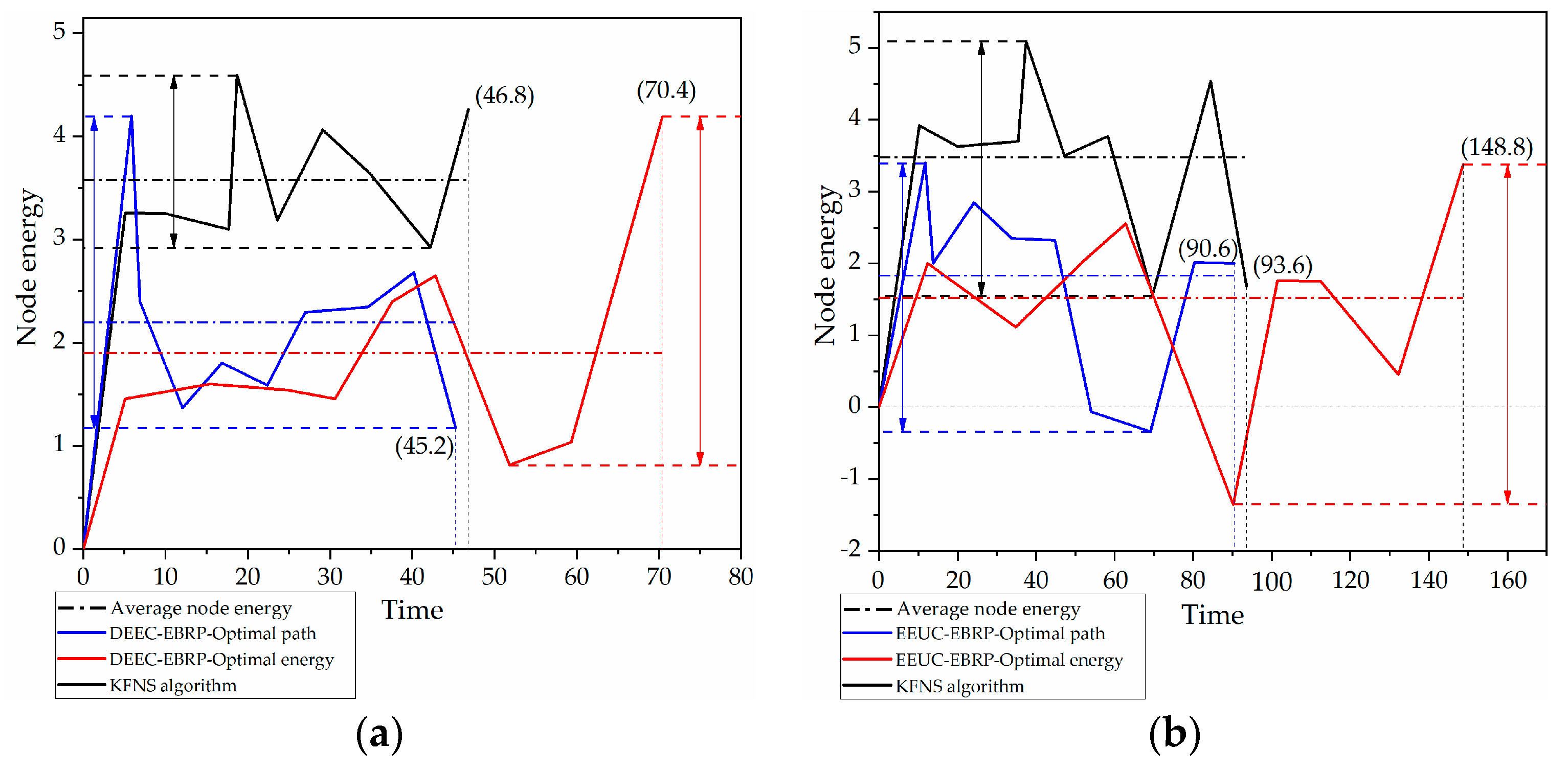
4.3. Recovery Phase Simulation
4.4. Node Recycling Process Simulation
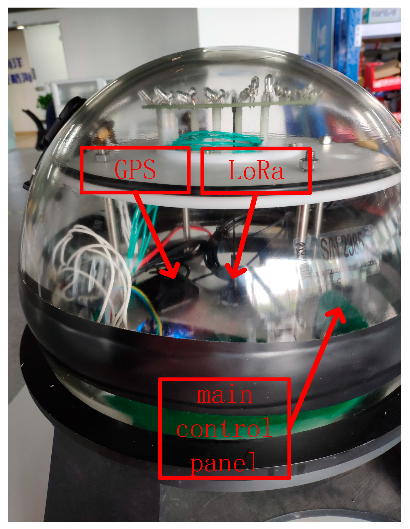
4.5. Implementation and Experiments
5. Conclusions
Author Contributions
Funding
Conflicts of Interest
References
- Chen:, J.; Zhang, W.; Wan, Z.; Li, S.; Huang, T.; Fei, Y. Oil spills from global tankers: Status review and future governance. J. Clean. Prod. 2019, 227, 20–32. [Google Scholar] [CrossRef]
- Beyer, J.; Trannum, H.C.; Bakke, T.; Hodson, P.V.; Collier, T.K. Environmental effects of the Deepwater Horizon oil spill: A review. Mar. Pollut. Bull. 2016, 110, 28–51. [Google Scholar] [CrossRef] [PubMed]
- Wang, X.; Wei, D.; Wei, X.; Cui, J.; Pan, M. HAS(4): A Heuristic Adaptive Sink Sensor Set Selection for Underwater AUV-Aid Data Gathering Algorithm. Sensors 2018, 18, 4110. [Google Scholar] [CrossRef] [PubMed]
- Izadi, D.; Abawajy, J.H.; Ghanavati, S.; Herawan, T. A data fusion method in wireless sensor networks. Sensors 2015, 15, 2964–2979. [Google Scholar] [CrossRef]
- Feng, T.; Li, W.; Hwang, M. False Data Report Filtering Scheme in Wireless Sensor Networks: A Survey. Int. J. Netw. Secur. 2015, 17, 229–236. [Google Scholar]
- Xu, G.; Shi, Y.; Sun, X.; Shen, W. Internet of Things in Marine Environment Monitoring: A Review. Sensors 2019, 19, 1711. [Google Scholar] [CrossRef] [PubMed]
- Han, G.; Liu, L.; Chan, S.; Yu, R.; Yang, Y. HySense: A hybrid mobile crowdsensing framework for sensing opportunities compensation under dynamic coverage constraint. IEEE Commun. Mag. 2017, 55, 93–99. [Google Scholar] [CrossRef]
- Moroni, D.; Pieri, G.; Salvetti, O.; Tampucci, M.; Domenici, C.; Tonacci, A. Sensorized buoy for oil spill early detection. In Proceedings of the Oceans 2015—Genova, Genova, Italy, 18–21 May 2015; pp. 1–5. [Google Scholar]
- Xu, J.; Liu, P.; Wang, H.; Lian, J.; Li, B. Marine Radar Oil Spill Monitoring Technology Based on Dual-Threshold and C-V Level Set Methods. J. Indian Soc. Remote Sens. 2018, 46, 1949–1961. [Google Scholar] [CrossRef]
- Sun, S.; Hu, C. The Challenges of Interpreting Oil-Water Spatial and Spectral Contrasts for the Estimation of Oil Thickness: Examples from Satellite and Airborne Measurements of the Deepwater Horizon Oil Spill. IEEE Trans. Geosci. Remote Sens. 2019, 57, 2643–2658. [Google Scholar] [CrossRef]
- Yu, F.; Hu, X.; Dong, S.; Liu, G.; Zhao, Y.; Chen, G. Design of a low-cost oil spill tracking buoy. J. Mar. Sci. Technol. 2018, 23, 188–200. [Google Scholar] [CrossRef]
- Wu, H.; Mei, X.; Chen, X.; Li, J.; Wang, J.; Mohapatra, P. A novel cooperative localization algorithm using enhanced particle filter technique in maritime search and rescue wireless sensor network. ISA Trans. 2018, 78, 39–46. [Google Scholar] [CrossRef] [PubMed]
- Wu, H.; Xian, J.; Wang, J.; Khandge, S.; Mohapatra, P. Missing data recovery using reconstruction in ocean wireless sensor networks. Comput. Commun. 2018, 132, 9. [Google Scholar] [CrossRef]
- Zou, T.; Li, Z.; Li, S.; Lin, S. Adaptive Energy-Efficient Target Detection Based on Mobile Wireless Sensor Networks. Sensors 2017, 17, 1028. [Google Scholar]
- Huang, M.; Liu, A.; Xiong, N.; Wang, T.; Vasilakos, A.V. A Low-Latency Communication Scheme for Mobile Wireless Sensor Control Systems. IEEE Trans. Syst. Man Cybern. Syst. 2019, 49, 317–332. [Google Scholar] [CrossRef]
- Chandrawanshi, V.S.; Tripathi, R.; Pachauri, R. An intelligent energy efficient clustering technique for multiple base stations positioning in a wireless sensor network. J. Intell. Fuzzy Syst. 2019, 36, 2409–2418. [Google Scholar] [CrossRef]
- He, S.; Chen, J.; Jiang, F.; Yau, D.K.Y.; Xing, G.; Sun, Y. Energy Provisioning in Wireless Rechargeable Sensor Networks. IEEE Trans. Mob. Comput. 2013, 12, 1931–1942. [Google Scholar] [CrossRef]
- Han, G.; Liu, L.; Jiang, J.; Shu, L.; Hancke, G. Analysis of energy-efficient connected target coverage algorithms for industrial wireless sensor networks. IEEE Trans. Ind. Inform. 2015, 13, 135–143. [Google Scholar] [CrossRef]
- Chen, J.; Li, J.; Lai, T. Trapping Mobile Targets in Wireless Sensor Networks: An Energy-Efficient Perspective. IEEE Trans. Veh. Technol. 2013, 62, 3287–3300. [Google Scholar] [CrossRef]
- Yousefi, H.; Malekimajd, M.; Ashouri, M.; Movaghar, A. Fast aggregation scheduling in wireless sensor networks. IEEE Trans. Wirel. Commun. 2015, 14, 3402–3414. [Google Scholar] [CrossRef]
- Shurman, M.M.; Al-Mistarihi, M.F.; Harb, S. An Energy-Efficient Coverage Aware Clustering Mechanism for Wireless Sensor Networks. In Proceedings of the 5th International Conference on Communications, Computers and Applications (MIC-CCA 2012), Istanbul, Turkey, 12–14 October 2012; pp. 154–158. [Google Scholar]
- Shurman, M.M.; Al-Mistarihi, M.F.; Alsaedeen, M.; Drabkh, K.; Ababnah, A. Hierarchal Clustering Using Genetic Algorithm in Wireless Sensor Networks. In Proceedings of the 36th International Convention on Information and Communication Technology, Electronics and Microelectronics (MIPRO2013), Opatija, Croatia, 20–24 May 2013; pp. 479–483. [Google Scholar]
- Yin, K.; Zhong, C. Data collection in wireless sensor networks. In Proceedings of the IEEE International Conference on Cloud Computing and Intelligence Systems, Beijing, China, 15–17 September 2011; pp. 98–102. [Google Scholar]
- Lu, J.; Zhang, B.; Xu, L. A data correlation-based wireless sensor network clustering algorithm. In Proceedings of the 2010 International Conference on Computer Application and System Modeling (ICCASM 2010), Taiyuan, China, 22–24 October 2010; pp. 61–65. [Google Scholar]
- Shurman, M.M.; Alomari, Z.M.; Mhaidat, K.M. An Efficient Billing Scheme for Trusted Nodes Using Fuzzy Logic in Wireless Sensor Networks. Wirel. Eng. Technol. 2014, 5, 62–73. [Google Scholar] [CrossRef]
- Hamzah, A.; Shurman, M.; Al-Jarrah, O.; Taqieddin, E. Energy-Efficient Fuzzy-Logic-Based Clustering Technique for Hierarchical Routing Protocols in Wireless Sensor Networks. Sensors 2019, 19, 561. [Google Scholar] [CrossRef] [PubMed]
- Heinzelman, W.B.; Chandrakasan, A.P.; Balakrishnan, H. An application-specific protocol architecture for wireless microsensor networks. IEEE Trans. Wirel. Commun. 2002, 1, 660–670. [Google Scholar] [CrossRef]
- Lindsey, S. PEGASIS: Power efficient gathering in sensor information systems. In Proceedings of the IEEE Aerospace Conference Proceedings, Big Sky, MT, USA, 9–16 March 2002; pp. 1125–1129. [Google Scholar]
- Ihsan, A.; Saghar, K.; Fatima, T.; Hasan, O. Formal comparison of LEACH and its extensions. Comput. Stand. Interfaces 2019, 62, 119–127. [Google Scholar] [CrossRef]
- Qing, L.; Zhu, Q.; Wang, M. Design of a distributed energy-efficient clustering algorithm for heterogeneous wireless sensor networks. Comput. Commun. 2006, 29, 2230–2237. [Google Scholar] [CrossRef]
- Ahmad, M.; Li, T.; Khan, Z.; Khurshid, F.; Ahmad, M. A Novel Connectivity-Based LEACH-MEEC Routing Protocol for Mobile Wireless Sensor Network. Sensors 2018, 18, 4278. [Google Scholar] [CrossRef] [PubMed]
- Li, C.; Ye, M.; Chen, G.; Wu, J. An energy-efficient unequal clustering mechanism for wireless sensor networks. In Proceedings of the IEEE International Conference on Mobile Adhoc and Sensor Systems Conference, Washington, DC, USA, 7–10 November 2005; pp. 597–604. [Google Scholar]
- Zhang, R.; Cao, J. Uneven Clustering Routing Algorithm for Wireless Sensor Networks Based on Ant Colony Optimization. J. Xi’An Jiaotong Univ. 2010, 44, 33–38. [Google Scholar]
- Ding, Y.; Ding, Y.; Yu, C.; Li, W. An Energy-Efficient Clustering Routing Algorithm with Improved Quality of Cluster in Wireless Sensor Networks. Chin. J. Sens. Actuators 2012, 25, 258–262. [Google Scholar]
- Park, G.Y.; Kim, H.; Jeong, H.W.; Youn, H.Y. A Novel Cluster Head Selection Method based on K-means Algorithm for Energy Efficient Wireless Sensor Network. In Proceedings of the 2013 27th International Conference on Advanced Information Networking and Applications Workshops, Barcelona, Spain, 25–28 March 2013; pp. 910–915. [Google Scholar]
- Sert, S.A.; Alchihabi, A.; Yazici, A. A Two-Tier Distributed Fuzzy Logic Based Protocol for Efficient Data Aggregation in Multihop Wireless Sensor Networks. IEEE Trans. Fuzzy Syst. 2018, 26, 3615–3629. [Google Scholar] [CrossRef]
- Jesudurai, S.A.; Senthilkumar, A. An improved energy efficient cluster head selection protocol using the double cluster heads and data fusion methods for IoT applications. Cogn. Syst. Res. 2019, 57, 101–106. [Google Scholar] [CrossRef]
- Li, L.; Li, D. An Energy-Balanced Routing Protocol for a Wireless Sensor Network. J. Sens. 2018, 5, 8505616. [Google Scholar] [CrossRef]
- Pamucar, D.; Ljubojevic, S.; Kostadinovic, D.; Dorovic, B. Cost and risk aggregation in multi-objective route planning for hazardous materials transportation-A neuro-fuzzy and artificial bee colony approach. Expert Syst. Appl. 2016, 65, 15. [Google Scholar] [CrossRef]
- Ebrahimi, H.; Milos, T. Optimization of dangerous goods transport in urban zone. Decis. Mak. Appl. Manag. Eng. 2018, 1, 131–152. [Google Scholar] [CrossRef]
- Zhang, L.; Yang, W.; Rao, Q.; Nai, W.; Dong, D. An energy saving routing algorithm based on Dijkstra in wireless sensor networks. J. Inf. Comput. Sci. 2013, 10, 2087–2096. [Google Scholar] [CrossRef]
- Razzaq, M.; Shin, S. Fuzzy-Logic Dijkstra-Based Energy-Efficient Algorithm for Data Transmission in WSNs. Sensors 2019, 19, 1040. [Google Scholar] [CrossRef] [PubMed]
- Simon, M.; Iveta, D.L.; Huraj, L.; Pospichal, J. Multi-Hub Location Heuristic for Alert Routing. IEEE Access 2019, 7, 40369–40379. [Google Scholar] [CrossRef]
- Periyasamy, S.; Khara, S.; Thangavelu, S. Balanced Cluster Head Selection Based on Modified k-Means in a Distributed Wireless Sensor Network. Int. J. Distrib. Sens. Netw. 2016, 12, 5040475. [Google Scholar] [CrossRef]
- Arjunan, S.; Sujatha, P. Lifetime maximization of wireless sensor network using fuzzy based unequal clustering and ACO based routing hybrid protocol. Appl. Intell. 2018, 48, 2229–2246. [Google Scholar] [CrossRef]
- Shelby, Z.; Pomalaza-Ráez, C.; Karvonen, H.; Haapola, J. Energy Optimization in Multihop Wireless Embedded and Sensor Networks. Int. J. Wirel. Inf. Netw. 2005, 12, 11–21. [Google Scholar] [CrossRef]
- Guezouli, L.; Barka, K.; Bouam, S.; Bouhta, D.; Aouti, S. Mobile sensor nodes collaboration to optimize routing process based mobility model. In Proceedings of the 2017 International Conference on Wireless Networks and Mobile Communications (WINCOM), Rabat, Morocco, 1–4 November 2017; pp. 1–5. [Google Scholar]
- Rida, M.; Makhoul, A.; Harb, H.; Laiymani, D.; Barharrigi, M. EK-means: A new clustering approach for datasets classification in sensor networks. Ad. Hoc. Netw. 2019, 3, 158–169. [Google Scholar] [CrossRef]
- Han, G.; Yang, X.; Liu, L.; Zhang, W. A joint energy replenishment and data collection algorithm in wireless rechargeable sensor networks. IEEE Internet Things J. 2018, 5, 2596–2604. [Google Scholar] [CrossRef]
- Zhu, E.; Li, P.; Ma, Z.; Li, X.; Liu, F. Effective and Optimal Clustering Based on New Clustering Validity Index. In Proceedings of the 2018 IEEE 22nd International Conference on Computer Supported Cooperative Work in Design (CSCWD), Nanjing, China, 9–11 May 2018; pp. 529–534. [Google Scholar]
- Zhang, M.; Duan, K. Improved Research to K-means Initial Cluster Centers. In Proceedings of the 2015 Ninth International Conference on Frontier of Computer Science and Technology, Dalian, China, 26–28 August 2015; pp. 349–353. [Google Scholar]
- Ioffe, S.; Szegedy, C. Batch normalization: Accelerating deep network training by reducing internal covariate shift. arXiv 2015, arXiv:1502.03167. [Google Scholar]


| Energy | |||
|---|---|---|---|
| Low | Close | Close | Close |
| Medium | Medium | Medium | Medium |
| High | Far | Far | Far |
| No. | Input | Output | ||||
|---|---|---|---|---|---|---|
| Energy | Weight | CH | ||||
| 1 | Low | Close | Close | Close | Low | HMid |
| 2 | Low | Close | Medium | Medium | HMid | Mid |
| 3 | Low | Close | Far | Far | High | LMid |
| 4 | Low | Medium | Close | Close | Low | LMid |
| 5 | Low | Medium | Medium | Medium | LMid | Low |
| 6 | Low | Medium | Far | Far | Mid | VLow |
| 7 | Low | Far | Close | Close | VLow | LMid |
| 8 | Low | Far | Medium | Medium | VLow | Low |
| 9 | Low | Far | Far | Far | Low | VLow |
| 10 | Medium | Close | Close | Close | HMid | High |
| 11 | Medium | Close | Medium | Medium | High | HMid |
| 12 | Medium | Close | Far | Far | VHigh | Mid |
| 13 | Medium | Medium | Close | Close | HMid | Mid |
| 14 | Medium | Medium | Medium | Medium | High | LMid |
| 15 | Medium | Medium | Far | Far | VHigh | Low |
| 16 | Medium | Far | Close | Close | VLow | LMid |
| 17 | Medium | Far | Medium | Medium | Low | Low |
| 18 | Medium | Far | Far | Far | LMid | VLow |
| 19 | High | Close | Close | Close | Mid | VHigh |
| 20 | High | Close | Medium | Medium | HMid | High |
| 21 | High | Close | Far | Far | VHigh | HMid |
| 22 | High | Medium | Close | Close | Mid | HMid |
| 23 | High | Medium | Medium | Medium | High | Mid |
| 24 | High | Medium | Far | Far | VHigh | LMid |
| 25 | High | Far | Close | Close | Low | High |
| 26 | High | Far | Medium | Medium | LMid | Mid |
| 27 | High | Far | Far | Far | HMid | LMid |
| Parameter Name | Parameter Value |
|---|---|
| Single-hop network size | |
| Multi-hop network size | |
| Number of nodes | 100 |
| Initial energy | , |
| Communication range of sensors | 60 m |
| Time for each round | 10 s |
| Speed range () | 1–5 m/s |
| Energy consumption of transmission circuit | 50 |
| Amplifier parameter for free-space model | 10 |
| Amplifier parameter for multi-path model | 0.0013 |
© 2019 by the authors. Licensee MDPI, Basel, Switzerland. This article is an open access article distributed under the terms and conditions of the Creative Commons Attribution (CC BY) license (http://creativecommons.org/licenses/by/4.0/).
Share and Cite
Zhang, Z.; Qi, S.; Li, S. Marine Observation Beacon Clustering and Recycling Technology Based on Wireless Sensor Networks. Sensors 2019, 19, 3726. https://doi.org/10.3390/s19173726
Zhang Z, Qi S, Li S. Marine Observation Beacon Clustering and Recycling Technology Based on Wireless Sensor Networks. Sensors. 2019; 19(17):3726. https://doi.org/10.3390/s19173726
Chicago/Turabian StyleZhang, Zhenguo, Shengbo Qi, and Shouzhe Li. 2019. "Marine Observation Beacon Clustering and Recycling Technology Based on Wireless Sensor Networks" Sensors 19, no. 17: 3726. https://doi.org/10.3390/s19173726
APA StyleZhang, Z., Qi, S., & Li, S. (2019). Marine Observation Beacon Clustering and Recycling Technology Based on Wireless Sensor Networks. Sensors, 19(17), 3726. https://doi.org/10.3390/s19173726